Impacts of boundary layer turbulence and land surface process parameterizations on simulated sea breeze characteristics

(1)

Geophysicae

Impacts of boundary layer turbulence and land surface process

parameterizations on simulated sea breeze characteristics

J.-F. Miao1, K. Wyser2, D. Chen3, and H. Ritchie4,5

1_{Key Laboratory of Meteorological Disaster of Ministry of Education, and College of Atmospheric Sciences, Nanjing}

University of Information Science and Technology, 219 Ningliu Road, Nanjing 210044, China

2_{Rossby Centre, Swedish Meteorological and Hydrological Institute (SMHI), 601 76 Norrk¨oping, Sweden} 3_{Department of Earth Sciences, University of Gothenburg, P.O. Box 460, 405 30 Gothenburg, Sweden} 4_{Department of Oceanography, Dalhousie University, 1355 Oxford Street, Halifax, NS, B3H 4J1, Canada} 5_{Meteorological Research Division, Environment Canada, 45 Alderney Drive, Dartmouth, NS B2Y 2N6, Canada}

Received: 21 October 2008 – Revised: 6 May 2009 – Accepted: 25 May 2009 – Published: 8 June 2009

Abstract. This paper investigates the sensitivity of sea breeze (SB) simulations to combinations of boundary-layer turbulence and land-surface process parameterizations im-plemented in the MM5 mesoscale meteorological mode for an observed SB case over the Swedish west coast. Var-ious combinations from four different planetary boundary layer (PBL) schemes [Blackadar, Gayno-Seaman (GS), Eta, MRF], and two land surface model (LSM) schemes (SLAB, Noah) with different complexity are designed to simulate a typical SB case over the Swedish west coast. The simula-tions are conducted using two-way interactively nested grids. Simulated 10-m winds are compared against observed near-surface wind data from the G ¨OTE2001 campaign to examine the diurnal cycle of wind direction and speed for SB tim-ing. The SB (vertical) circulation is also compared in the different experiments. The results show that the different combinations of PBL and LSM parameterization schemes re-sult in different SB timing and vertical circulation character-istics. All experiments predict a delayed SB. The vertical component of the SB circulation varies in the experiments, among which the GS PBL scheme produces the strongest SB circulation. Evident differences between the SLAB and Noah LSMs are also found, especially in maximum of up-draft and downup-draft velocities of the SB vertical circulation. The results have significant implications for convective ini-tiation, air quality studies and other environmental problems in coastal areas.

Correspondence to: J.-F. Miao

([email protected])

Keywords. Atmospheric composition and structure (Biosphere-atmosphere interactions; Evolution of the atmosphere) – Meteorology and atmospheric dynamics (Mesoscale meteorology; Turbulence)

1 Introduction

Sea breeze (SB) is an important mesoscale meteorological phenomenon in coastal areas caused by a thermal difference between sea and land during the daytime. It is a main fea-ture of surface heterogeneities which force mesoscale at-mospheric circulations, and has been studied observation-ally, experimentobservation-ally, theoretically and numerically for a long time (Abbs and Physick, 1992; Simpson, 1994; Miller et al., 2003).

Also, SB is the prototypical mesoscale circulation and was the first to be simulated in numerical models (Angevine et al., 2006). Its theoretical background is well understood and simple enough, but real SB is very sensitive to real envi-ronmental complexity, surface temperature, and large scale background flow (Zhong and Takle, 1993; Angevine et al., 2006). SB circulation plays an important role in air pollution transport and dispersion (Ding et al., 2004; Oh et al., 2006). It affects human activities not only along the coast but also further inland. Therefore, SB study is still an interesting and challenging subject (Miao et al., 2003; Angevine et al., 2006; Drobinski et al., 2006; Prtenjak and Grisogono, 2007; Srini-vas et al., 2007).

(2)

2304 J.-F. Miao et al.: Impacts of boundary layer turbulence and land surface process parameterizations meteorological fields (weather data) are used as input to air

quality models, small errors in meteorological simulations, which may be of minor concern for weather forecasting, may nevertheless lead to erroneous air quality predictions (Zhong et al., 2007). Previous studies have suggested the importance of understanding SB timing in pollutant transport and accu-mulation in coastal areas (e.g., Ding et al., 2004; Oh et al., 2006). The results have shown that late onset of SB-induced stagnant conditions in the morning allows pollutant concen-tration to build up and enhances ozone accumulation in the afternoon. The delayed SB can contribute to the daytime transport of pollution and high ozone on the coast (Ding et al., 2004).

Over the past years, the SB has been extensively studied over the Swedish west coast with a focus on observational analyses (Gustavsson et al., 1995; Borne et al., 1998) to im-prove our understanding of this meteorological phenomenon. Nevertheless, to our knowledge, very few modelling efforts over this area can be found in the literature. With the de-velopment of the study of air pollution dynamics, SB simu-lations at high resolutions over this area, where the second largest city (Gothenburg) in Sweden is located, are needed to understand SB dynamics at fine scales and its implications for air pollution transport and dispersion.

The turbulence parameterization, or PBL parameteriza-tion, is one of most important model components in the me-teorological and air quality models (Pleim, 2007). It ac-counts for the vertical mixing of atmospheric fields induced by small-scale turbulent motions, which are usually not re-solved on the model grid (Z¨angl et al., 2008), and is very important for accurate simulations of boundary-layer tem-perature, humidity, wind, and mixed-layer depth (Berg and Zhong, 2005).

The land surface model (LSM), in which land-surface pro-cesses are parameterized, provides surface sensible and latent heat fluxes as lower boundary conditions to coupled atmo-spheric model. These heat and moisture fluxes are then trans-ported throughout the planetary boundary layer (PBL) and interact with other model physics including cloud, radiation and precipitation processes (Chen and Dudhia, 2001b). In other words, surface heat, moisture, momentum fluxes, and short and long wave radiations are the primary factors driving the development of the turbulent boundary layer (Seaman, 2000). Also, the advection of cold and moist air by SB can lead to important modifications to the land surface fluxes, and thus have consequences on the boundary layer development. The previous studies have shown that the simulation of SB circulation caused by land-sea air temperature contrast is closely linked to boundary-layer turbulence and land-surface processes simulations. For example, Prtenjak and Grisogono (2002) investigated the influence of land surface roughness length on the strength of SB circulation, and found that very rough surfaces weaken the SB circulation during the day, causing a slower inland penetration. In turn, the enhanced turbulent fluxes cause onset of the SB circulation earlier

(Malda et al., 2007). Miao et al. (2003) examined the im-pact of land degradation (desertification) on the SB circula-tion characteristics by using the Regional Atmospheric Mod-elling System (RAMS) model, suggesting that land degrada-tion (land cover change and soil moisture decrease) results in an enhanced SB circulation and significantly influences the SB pattern and magnitude.

The MM5 mesoscale meteorological model (Grell et al., 1995) is a limited-area, non-hydrostatic, terrain-following sigma-coordinate primitive equation model designed to sim-ulate or predict mesoscale atmospheric circulations, and it has been widely applied in operational numerical weather forecasting (Zhong et al., 2005; Akylas et al., 2007) and air quality studies (e.g., Ding et al., 2004; Miao, 2006; Miao et al., 2006, 2008; Mao et al., 2006; Bossioli et al., 2009). It is also increasingly used in SB modelling (e.g., Colby, 2004; Zhu and Atkinson, 2004; Oh et al., 2006; Srinivas et al., 2007; Dandou et al., 2009a). This model provides model-ers with many options of physical parameterization schemes for cumulus convection, microphysics, radiation, PBL tur-bulence, and land surface processes. Among the various parameterizations representing different physical processes, PBL and LSM parameterizations are especially important for simulations of atmospheric properties and local circulations (Zhong et al., 2007), and thus have critical implications for air quality simulations (P´erez et al., 2006; Pleim, 2007).

(3)

[image:3.595.141.453.87.198.2]

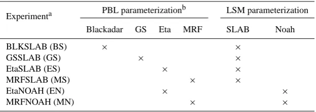
Table 1. Summary of numerical experiments.

Experimenta PBL parameterization

b _{LSM parameterization}

Blackadar GS Eta MRF SLAB Noah

BLKSLAB (BS) × ×

GSSLAB (GS) × ×

EtaSLAB (ES) × ×

MRFSLAB (MS) × ×

EtaNOAH (EN) × ×

MRFNOAH (MN) × ×

a_{Abbreviations of the experiments are given in the parentheses.}

b_{Moist vertical diffusion is used in Blackadar and MRF PBLs; Thermal roughness length uses Zilitinkevich formulation in Blackadar and}

MRF PBLs.

well with observations of temperature, all simulations had significant errors in wind speed. The similar results are also found in Miao et al. (2008).

Of the above cited studies, only a few examined the im-pacts of PBL and/or LSM parameterization schemes on sim-ulated SB (e.g., Srinivas et al., 2007; Zhong et al., 2007) and diurnal cycle of near-surface wind (e.g., Zhang and Zheng, 2004; Miao et al., 2008) despite the fact that SB is a proto-typical mesoscale circulation and that diurnal cycle of winds has significant implications for air quality studies.

The above-mentioned limitations and motivations lead to this study. The purpose is to simulate the SB at high res-olutions using the MM5 model and to study the sensitiv-ity of simulated SB characteristics, in particular timing and strength, to different combinations of PBL and LSM param-eterization schemes in the model. The results are then com-pared against the measurement data from the G ¨OTE2001 field campaign (Borne et al., 2005).

As an extension and supplement to Miao et al. (2008), this study focuses on the applications of MM5 mesoscale model to SB simulation, and includes one PBL scheme which was not examined there.

2 Model setup and numerical experiments

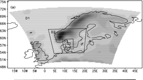
The model is set up with four two-way nested domains (D1, D2, D3, and D4) with horizontal grid spacing of 54, 18, 6, 2-km, respectively (Fig. 1a). D1 is used to simulate the large scale meteorological conditions. The inner three do-mains with increasingly finer resolution are used to capture mesoscale and local scale features. The innermost domain (D4) is the area of interest (Fig. 1b). There is a remarkable sea-land contrast in D4, and the coastline is in an approxi-mately north-south direction. All domains have 35 vertical full sigma levels and the model top is at 100 hPa. To allow the model to resolve SB circulations at higher resolutions, about 18 levels (half-σ level) are set up within the lowest

2 km. The height of the lowest model level (half-σ layer) is about 10 m, representing the average over the lowest 20 m above the surface.

In this study, the four widely-used PBL parameterization schemes [Blackadar PBL scheme (Blackadar, 1976, 1979; Zhang and Anthes, 1982), Gayno-Seaman (GS) PBL scheme (Shafran et al., 2000), Eta PBL scheme (Janji´c, 1990, 1994), and MRF PBL scheme (Hong and Pan, 1996)] and two LSM parameterization schemes [SLAB LSM (Dudhia, 1996) and Noah LSM (Chen and Dudhia, 2001a)] in MM5, Ver-sion 3.6.3, are chosen based on: (1) availability of coupling of PBL schemes and LSMs, and (2) that LSM can be cou-pled with more than one PBL scheme, in the model. Table 1 presents the different combinations of PBL and LSM param-eterizations used in the experiments.

(4)

2306 J.-F. Miao et al.: Impacts of boundary layer turbulence and land surface process parameterizations

37

(a)

(b)

Fig. 1. (a) Modelling domains and grid configuration. Domains 1,

2, 3, and 4 (denoted by D1, D2, D3 and D4) have a horizontal grid resolution of 54, 18, 6 and 2 km, respectively. Four domains

consist of 50×50, 64×55, 62×52, and 40×46 horizontal gridcells

(N-S direction by E-W direction), respectively. Innermost domain refers to D4. Shaded is model terrain (in meters) with 54-km grid resolution for D1; (b) Zooming-in model area of interest (D4) and model terrain (shaded in meters) with 2-km grid resolution, as well as locations of observational sites by letters: K (Kanotf¨oreningen),

R (Risholmen), J (J¨arnbrott), A ( ˚Aby), G (GVC), L (Lejonet), T

(Tagene), S (S¨ave), TL (Trubaduren), and LV (Landvetter). Dashed line indicates location of the vertical cross-section used in this study

(along 57.72◦N).

Also, of the two LSM schemes chosen, the SLAB LSM is a simple LSM while the Noah LSM is an advanced LSM. In this study, the SLAB LSM consists of: (1) a five-layer soil temperature model (Dudhia, 1996), and (2) a bucket soil moisture model (Manabe, 1969). The model is used to pre-dict the soil temperature in the five layers with thickness from top to bottom of 1, 2, 4, 8 and 16 cm, and keeps a budget of soil moisture allowing moisture availability to vary with time in response to rainfall and evaporation rates. The Noah LSM is used to predict soil moisture and temperature in four layers with thickness from top to bottom of 10, 30, 60 and 100 cm, as well as canopy moisture and water-equivalent snow depth.

It uses soil and vegetation types in handling evapotranspira-tion. The dominant vegetation type in each grid is selected to represent the grid vegetation characteristics when the model horizontal grid resolution is larger than 1 km×1 km.

The other physics options used in this study are: Anthes-Kuo convection scheme in D1 and Kain-Fritsch convection including shallow convection (KF2; Kain, 2004) in D2–D4. It is necessary to mention that convection parameterization is also applied in D4 with less than 5 km grid spacing as the KF2 scheme has been updated recently and also includes shallow convection for a potential improvement at higher res-olutions (also refer to B´elair and Mailhot, 2001). The Dudhia simple ice microphysics scheme (Dudhia, 1989), Rapid Ra-diative Transfer Model (RRTM) longwave scheme (Mlawer et al., 1997) and Dudhia cloud-radiation shortwave scheme (Dudhia, 1989) are used for all domains.

The initial and boundary conditions were taken from the European Center for Medium-Range Weather Forecasts (ECMWF) operational analysis archive data with a spatial resolution of 0.5◦ by 0.5◦ and a temporal resolution of six hours. The USGS 25-category land use data and terrain data, as well as global 17-category soil type data are used. The topography for the coarse domain (D1) with 54 km×54 km resolution is shown in Fig. 1a, while that for the innermost domain (D4) with 2 km×2 km is shown in Fig. 1b. As seen from Fig. 1b, the terrain height in D4 varies from a few me-ters near the coastal lines to about 200 m over the inland ar-eas. Moreover, soil moisture is initialized for the LSMs using the ECMWF data.

The 48-h simulations for all numerical experiments are performed, starting from 00:00 UTC 7 May 2001 with model output at one-hour intervals. The first 24 h are discarded as model spin-up, while the last 24-h simulation results are ana-lyzed as the second day of the simulations (8 May 2001) has been identified as a typical SB case from the observations during the G ¨OTE2001 field campaign (Borne et al., 2005).

3 G ¨OTE2001 data and analysis methods

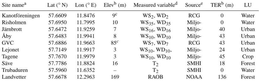
[image:4.595.51.285.63.194.2]

(5)

[image:5.595.91.505.100.232.2]

Table 2. Name, location and other information for observational sites used in this study (Lat: latitude, Lon: longitude, Elev: elevation), as

well as model terrain (TER) height and dominant land use (LU) represented in 2-km resolution (D4) closest to observational sites.

Site namea Lat (◦N) Lon (◦E) Elevb(m) Measured variabled Sourcee TERb(m) LU

Kanotf¨oreningen 57.6609 11.8476 9c WS2, WD2 RCG 0 Water

Risholmen 57.6950 11.7995 10 WS35, WD35 Miljo- 0 Water

J¨arnbrott 57.6472 11.9259 7 WS16, WD16 Miljo- 40 Urban

˚

Aby 57.6483 11.9941 8 WS10, WD10 Miljo- 43 Urban

GVC 57.6886 11.9663 85c WS7, WD7 RCG 43 Urban

Lejonet 57.7149 11.9917 3 WS10, WD10, Miljo- 24 Urban

Tagene 57.7670 11.9979 3 WS₁₀, WD₁₀ Miljo- 45 Crop

S¨ave 57.7786 11.8824 16 T2 SMHI 18 Forest

Trubaduren 57.5960 11.6352 – T₂ SMHI 0 Water

Landvetter 57.6678 12.2963 169 RAOB NOAA 136 Forest

a_{Refer to Fig. 1b for the locations in D4. J¨arnbrott is a mast site, and the first level for wind measurement is at 16 m high. S¨ave is a routine}

weather station, and Landvetter is a radiosounding station; Trubaduren is a lighthouse station.

b_{Unit: meters ASL (Above Sea Level)}

c_{Height of mounted measurement mast from the sea level to the roof. For Kanotf¨oreningen, the elevation is 3 m, and the building height is}

6 m; For GVC, the elevation is 60 m, and the building height is 25 m.

d_{WS: wind speed; WD: wind direction. Subscript represents the measured height above ground level (a.g.l.) or above the roof; RAOB:}

radiosounding; Hourly data for all sites except for S¨ave, Trubaduren and Landvetter (3-h time intervalT2at S¨ave and Trubaduren, and 12-h

time interval RAOB at Landvetter).

e_{Miljo-: Environment Administration, City of Gothenburg; RCG: Regional Climate Group; SMHI: Swedish Meteorological and}

Hydrolog-ical Institute.

is used to represent synoptic-scale background flow. On 8 May 2001, the Swedish west coast was dominated by a high pressure system. The synoptic-scale background wind is southeasterly (5.7 m s−1), easterly (6.2 m s−1), and southerly (7.2 m s−1) at 00:00 UTC, 12:00 UTC, and 24:00 UTC, re-spectively (Miao, 2006). The flow is an offshore synoptic wind during the daytime, and thus favors SB development (Zhong and Takle, 1993; Miao et al., 2003). Also, the ob-served cloud cover data at the S¨ave site shows that 8 May 2001 is a clear sky day (Miao et al., 2008), and hence the SB event chosen is a clear-sky SB case.

4 Sea breeze timing and strength

In this study, the observed near-surface wind data from the campaign is used to compare with the simulated near-surface wind (10 m a.g.l.) at the closest grid point from D4 with 2-km grid spacing. The simulated 10-m wind is not adjusted ver-tically to the measurement heights, although there are some differences between the model levels and the measurement heights (Miao et al., 2008). It is noted that surface measure-ment represents a value only at a given horizontal location and height, while the simulated result represents a volume-averaged value.

To examine the impacts of different combinations of PBL and LSM parameterization schemes on simulated SB in tim-ing, “SB timing” is characterized at certain sites in this study by three feature parameters (cf. Prezerakos, 1986): SB

on-set (τs), SB end time (“cessation”) (τe), and the time (τmax)

when the near-surface wind speed reaches a first peak value during the daytime. The value of wind speed at timeτmaxis defined as “SB strength” in this study.

Theτs is defined according to the following criteria that must all be fulfilled: 1) there is sharp change in wind direc-tion (greater than 30◦) around timeτs; 2) the wind direction at timeτs is in the range of 180◦to 360◦; 3) the wind speed at timeτs+1 is greater than that at timeτs. These three cri-teria must be met concurrently. Theτe is reached if any of the following criteria is met: 1) the wind direction at time

τe is in the range of 180◦ to 360◦, but that at timeτe+1 is beyond the range of 180◦_{to 360}◦_{; The wind speed at time}

τe is less than that at timeτe−1 orτe+1; 2) the wind direc-tion at timeτe−1 is in the range of 180◦to 360◦; The wind speed at timeτe is less than that at timeτe−1, and less than or equal to 0.5 m s−1. Also, during the daytime the wind has to be onshore for at least 2 consecutive hours for recognizing and defining SB onset and cessation (cf. Furberg et al., 2002; Prtenjak and Grisogono, 2007).

(6)

[image:6.595.138.455.90.360.2]

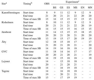
Table 3. Observed (OBS) and simulated sea breeze timing (o’clock) with different experiments at all observational sites on 8 May 2001.

Sitea Timingb OBS Experiment

c

BS GS ES MS EN MN

Kanotf¨oreningen Start time 8 9 11 12 9 12 9

End time 21 20 21 21 22 20 20

Time of max SB 15 16 15 15 15 15 15

Risholmen Start time 8 10 11 12 9 12 9

End time 20 21 21 21 22 20 19

Time of max SB 14 15 15 15 16 15 15

J¨arnbrott Start time 11 14 13 15 15 18 15

End time 20 20 21 20 21 20 20

Time of max SB 13 19 15 17 20 19 19

˚

Aby Start time 12 18 15 18 17 – 17

End time 21 20 21 20 21 – 20

Time of max SB 14 19 16 18 18 – 19

GVC Start time 11 18 14 16 17 – 17

End time 20 20 21 20 21 – 19

Time of max SB 14 19 15 18 18 – 18

Lejonet Start time 14 – 15 18 18 – –

End time 20 – 21 20 21 – –

Time of max SB 14 – 16 19 18 – –

Tagene Start time 14 – 16 18 18 – –

End time 19 – 20 21 21 – –

Time of max SB 15 – 17 19 19 – –

a_{The observational sites from top to bottom are sorted by the relative distance to the coastline from near to far. All sites are within the}

distance of less than 16 km to coastline.

b_{See the text for definitions; Time of max SB: Occurrence time of Maximum SB; Unit: O’clock (UTC).}

c_{Refer to Table 1 for abbreviations of the experiments.}

Table 4. Observed (OBS) and simulated sea breeze strengthwith

different experiments at all observational sites on 8 May 2001. Sea breeze strength is defined as the first peak value of observed and simulated near-surface wind speed during SB hours (cf. Table 3).

Sitea OBS Experiment

b

BS GS ES MS EN MN

Kanotf¨oreningen 5.1 6.0 5.4 6.1 3.8 6.4 4.1 Risholmen 8.2 4.9 4.9 5.7 3.7 4.9 3.3 J¨arnbrott 4.2 3.4 2.9 2.6 2.3 1.7 2.5

˚

Aby 4.1 3.0 3.0 2.0 2.2 – 2.7 GVC 4.5 2.3 2.9 2.3 2.2 – 2.1 Lejonet 3.7 – 3.3 1.9 2.5 – – Tagene 4.8 – 3.6 2.0 2.4 – –

a_{Refer to the note}a_{of Table 3.}

b_{Refer to Table 1 for abbreviations of the experiments.}

convenience of discussion, the seven observational sites are classified into coastal sites (Kanotf¨oreningen, Risholmen) and inland sites (J¨arnbrott, ˚Aby, GVC, Lejonet, Tagene). This classification is mainly based on the distance of the sites to the coastline and the dominant land use at the model grid-cells (cf. Fig. 1b and Table 2).

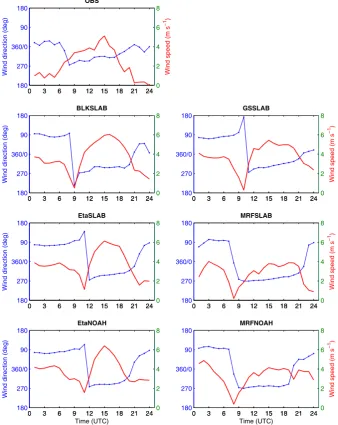
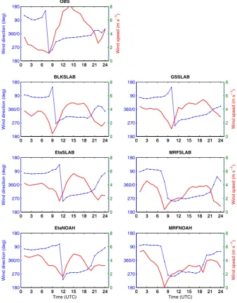
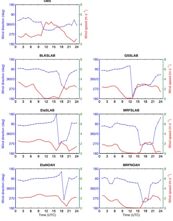
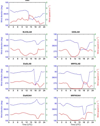
As seen from Figs. 2, 3, at the coastal sites all experiments capture the observed SB, but the predicted SB onset shows large differences (Table 3). Compared to the observed SB on-set, the predicted SB onset lags 1 to 4 h at Kanotföreningen and Risholmen sites. Among all experiments, MRFSLAB and MRFNOAH show the best performance in reproducing the observed SB onset, while EtaSLAB and EtaNOAH are the poorest. The BLKSLAB shows the same performance as MRFSLAB and MRFNOAH at Kanotföreningen, but a little poorer than MRFSLAB and MRFNOAH at Risholmen. The difference in the predicted SB end time among various exper-iments is not significant, and there is only−1 to 2 h lag from the observed SB end time at Kanotföreningen, and 1 h lag at Risholmen. Consequently, the simulated SB life span with different experiments displays large differences. It ranges from 8 to 13 h at Kanotföreningen (observed: 13 h), and from 8 to 11 h at Risholmen (observed: 12 h). Further, the simu-lated SB strength is highly variable among the experiments (Table 4). It varies from 3.8 to 6.4 m s−1at Kanotföreningen, and 3.3 to 5.7 m s−1at Risholmen. The deviation from the observations amounts to−25 to 25% of observed SB strength at Kanotföreningen, and−59 to−30% at Risholmen.

[image:6.595.50.284.489.603.2]

(7)

38

0 3 6 9 12 15 18 21 24

180 270 360/0 90 180

Wind direction (deg)

0 3 6 9 12 15 18 21 240

2 4 6 8

BLKSLAB

0 3 6 9 12 15 18 21 24

180 270 360/0 90 180

0 3 6 9 12 15 18 21 240

2 4 6 8

Wind speed (m s

−

1)

GSSLAB

0 3 6 9 12 15 18 21 24

180 270 360/0 90 180

0 3 6 9 12 15 18 21 240

2 4 6 8

EtaSLAB

0 3 6 9 12 15 18 21 24

180 270 360/0 90 180

0 3 6 9 12 15 18 21 240

2 4 6 8

Wind speed (m s

−

1)

MRFSLAB

0 3 6 9 12 15 18 21 24

180 270 360/0 90 180

0 3 6 9 12 15 18 21 240

2 4 6 8

Time (UTC)

EtaNOAH

0 3 6 9 12 15 18 21 24

180 270 360/0 90 180

0 3 6 9 12 15 18 21 240

2 4 6 8

Wind speed (m s

−

1)

Time (UTC)

MRFNOAH

0 3 6 9 12 15 18 21 24

180 270 360/0 90 180

0 3 6 9 12 15 18 21 240

2 4 6 8

Wind speed (m s

−

1)

OBS

934 935 936

Fig. 2 937

[image:7.595.129.468.67.493.2]

938 939 940 941

Fig. 2. Observed (OBS) and simulated hourly near-surface wind direction (dotted solid line) and wind speed (solid thick line) with different

experiments during the period from 01:00 to 24:00 UTC (8 May 2001) at Kanotf¨oreningen site. Observed near-surface wind is measured at height shown in Table 2. Simulated near-surface wind (10 m a.g.l.) is from the closest grid point to observational site from D4 with 2-km grid spacing. On 8 May 2001, sunrise time in G¨oteborg (study area) is 03:05 UTC, and sunset time is 19:14 UTC (http://www.timeanddate. com/worldclock/). LT (local time) = UTC+2 over the study area (D4).

[Local Time (LT): UTC+2 h] with a sudden change in wind direction from northwesterly to westerly in the observation (approximately 65 degrees of difference from 07:00 UTC to 08:00 UTC). The wind rotates anti-clockwise (“backing”) between 06:00 UTC and 08:00 UTC, and clockwise after-wards through the daytime. Generally, the SB rotates clock-wise at most sites, which is typical in the Northern Hemi-sphere due to the Coriolis force, but the anti-clockwise rota-tion is possible at some sites because of topographic features (Orli´c et al., 1988; Simpson, 1996; Prtenjak and Grisogono, 2007). As seen from Fig. 2, MRFSLAB and MRFNOAH

(8)

39

0 3 6 9 12 15 18 21 24

180 270 360/0 90 180

0 3 6 9 12 15 18 21 240

2 4 6 8

BLKSLAB

0 3 6 9 12 15 18 21 24

180 270 360/0 90 180

0 3 6 9 12 15 18 21 240

2 4 6 8

Wind speed (m s

−

1)

GSSLAB

0 3 6 9 12 15 18 21 24

180 270 360/0 90 180

0 3 6 9 12 15 18 21 240

2 4 6 8

EtaSLAB

0 3 6 9 12 15 18 21 24

180 270 360/0 90 180

0 3 6 9 12 15 18 21 240

2 4 6 8

Wind speed (m s

−

1)

MRFSLAB

0 3 6 9 12 15 18 21 24

180 270 360/0 90 180

0 3 6 9 12 15 18 21 240

2 4 6 8

Time (UTC)

EtaNOAH

0 3 6 9 12 15 18 21 24

180 270 360/0 90 180

0 3 6 9 12 15 18 21 240

2 4 6 8

Wind speed (m s

−

1)

Time (UTC)

MRFNOAH

0 3 6 9 12 15 18 21 24

180 270 360/0 90 180

0 3 6 9 12 15 18 21 240

2 4 6 8

Wind speed (m s

−

1)

OBS

942 943

Fig. 3 944

[image:8.595.128.467.65.498.2]

945 946 947 948

Fig. 3. Same as Fig. 2 but at Risholmen site.

wind direction around 09:00 UTC that is not displayed in the observations. Here it is necessary to point out that the wind at this site was measured at the height of 35 m a.g.l. (Table 2), and that model results do not show difference in simulated wind direction at this site between the two lowest model lev-els (10 m and 38 m) for any experiment in this study. Also, it could be speculated that differences in the sense of rotation of the wind vector between Kanotf¨oreningen and Risholmen sites, which are not seen in any of the model simulations, are probably due to differences in topography between both sites that are not captured by the model representation of orogra-phy.

For the inland sites, the simulated wind seems to be more complex than the observed, as shown in Figs. 4–8 and

(9)

40

0 3 6 9 12 15 18 21 24

180 270 360/0 90 180

0 3 6 9 12 15 18 21 240

2 4 6 8

BLKSLAB

0 3 6 9 12 15 18 21 24

180 270 360/0 90 180

0 3 6 9 12 15 18 21 240

2 4 6 8

Wind speed (m s

−

1)

GSSLAB

0 3 6 9 12 15 18 21 24

180 270 360/0 90 180

0 3 6 9 12 15 18 21 240

2 4 6 8

EtaSLAB

0 3 6 9 12 15 18 21 24

180 270 360/0 90 180

0 3 6 9 12 15 18 21 240

2 4 6 8

Wind speed (m s

−

1)

MRFSLAB

0 3 6 9 12 15 18 21 24

180 270 360/0 90 180

0 3 6 9 12 15 18 21 240

2 4 6 8

Time (UTC)

EtaNOAH

0 3 6 9 12 15 18 21 24

180 270 360/0 90 180

0 3 6 9 12 15 18 21 240

2 4 6 8

Wind speed (m s

−

1)

Time (UTC)

MRFNOAH

0 3 6 9 12 15 18 21 24

180 270 360/0 90 180

0 3 6 9 12 15 18 21 240

2 4 6 8

Wind speed (m s

−

1)

OBS

949 950

Fig. 4 951

[image:9.595.128.466.65.494.2]

952 953 954 955

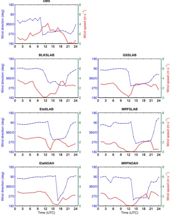
Fig. 4. Same as Fig. 2 but at J¨arnbrott site.

From the above result analyses, we may speculate that the Blackadar, GS and MRF PBL schemes display better perfor-mance in predicting SB timing at the most sites, while the Eta PBL scheme performs most poorly, no matter which LSM scheme it is coupled with (Table 3). This finding for Black-adar, GS, Eta and MRF PBLs from comparisons of BLK-SLAB, GSSALB, EtaSLAB and MRFBLK-SLAB, which are all coupled to the SLAB LSM, is consistent with that from the study of Srinivas et al. (2007).

Also, as seen from Figs. 2–8 and Table 3, the observed SB displays clear inland penetration, that is, SB onset (from early to late) varies with the distance of sites to the coastline (from near to far). However, the different experiments show highly varying performance in capturing SB inland

penetra-tion. The GSSLAB, EtaSLAB and MRFSLAB simulate the SB inland penetration reasonably well, but other combina-tions of PBL and LSM schemes lack the ability of reproduc-ing SB at further inland sites. Comparisons of EtaSLAB ver-sus EtaNOAH, and MRFSLAB verver-sus MRFNOAH indicate that the complexity of land surface model evidently affects SB simulations. This implies that land surface process pa-rameterization plays an important role in SB modelling.

(10)

41

0 3 6 9 12 15 18 21 24

180 270 360/0 90 180

0 3 6 9 12 15 18 21 240

2 4 6 8

BLKSLAB

0 3 6 9 12 15 18 21 24

180 270 360/0 90 180

0 3 6 9 12 15 18 21 240

2 4 6 8

Wind speed (m s

−

1)

GSSLAB

0 3 6 9 12 15 18 21 24

180 270 360/0 90 180

0 3 6 9 12 15 18 21 240

2 4 6 8

EtaSLAB

0 3 6 9 12 15 18 21 24

180 270 360/0 90 180

0 3 6 9 12 15 18 21 240

2 4 6 8

Wind speed (m s

−

1)

MRFSLAB

0 3 6 9 12 15 18 21 24

180 270 360/0 90 180

0 3 6 9 12 15 18 21 240

2 4 6 8

Time (UTC)

EtaNOAH

0 3 6 9 12 15 18 21 24

180 270 360/0 90 180

0 3 6 9 12 15 18 21 240

2 4 6 8

Wind speed (m s

−

1)

Time (UTC)

MRFNOAH

0 3 6 9 12 15 18 21 24

180 270 360/0 90 180

0 3 6 9 12 15 18 21 240

2 4 6 8

Wind speed (m s

−

1)

OBS

956 957

Fig. 5 958

[image:10.595.128.469.67.497.2]

959 960 961 962

Fig. 5. Same as Fig. 2 but at ˚Aby site.

5 Sensitivity of simulated sea breeze circulation charac-teristics to PBL and LSM parameterizations

SB vertical circulation characteristics are usually described by SB depth, inland penetration distance, and maximum horizontal wind speed, as well as maximum vertical ve-locity ahead of and behind the SB front (e.g., Gronas and Sandvik, 1998; Miao et al., 2003; Srinivas et al., 2007). Also, the distance-height cross-section ofU- (orV-) andW -component along latitude (or longitude) at a certain time is often used to illustrate and characterize SB vertical circula-tion, depending on the coastline direction. For this reason, we examine the X-Z cross section ofU- andW-component along latitude 57.72◦N (dashed line in Fig. 1b) at 15:00 UTC 8 May 2001 (Fig. 9), and extract or compute some major

characteristic parameters of the circulation, which are sum-marized in Table 5. These characteristics are used to quan-titatively distinguish the difference in simulated SB vertical circulation with different combinations of PBL and LSM pa-rameterization schemes.

(11)

42

0 3 6 9 12 15 18 21 24

180 270 360/0 90 180

0 3 6 9 12 15 18 21 240

2 4 6 8

BLKSLAB

0 3 6 9 12 15 18 21 24

180 270 360/0 90 180

0 3 6 9 12 15 18 21 240

2 4 6 8

Wind speed (m s

−

1)

GSSLAB

0 3 6 9 12 15 18 21 24

180 270 360/0 90 180

0 3 6 9 12 15 18 21 240

2 4 6 8

EtaSLAB

0 3 6 9 12 15 18 21 24

180 270 360/0 90 180

0 3 6 9 12 15 18 21 240

2 4 6 8

Wind speed (m s

−

1)

MRFSLAB

0 3 6 9 12 15 18 21 24

180 270 360/0 90 180

0 3 6 9 12 15 18 21 240

2 4 6 8

Time (UTC)

EtaNOAH

0 3 6 9 12 15 18 21 24

180 270 360/0 90 180

0 3 6 9 12 15 18 21 240

2 4 6 8

Wind speed (m s

−

1)

Time (UTC)

MRFNOAH

0 3 6 9 12 15 18 21 24

180 270 360/0 90 180

0 3 6 9 12 15 18 21 240

2 4 6 8

Wind speed (m s

−

1)

OBS

963 964

Fig. 6 965

[image:11.595.128.468.66.501.2]

966 967 968 969

Fig. 6. Same as Fig. 2 but at GVC site.

SB circulation with the largest inland penetration distance (20 km), SB depth (500 m), U-component (6.7 m s−1), up-draft and downup-draft velocities (67.6 cm s−1, 20.0 cm s−1), and SBCI index (5.87 m2s−2). Srinivas et al. (2007) have shown that GSSLAB predicts the most intensive SB front among all experiments (BLKSLAB, GSSLAB, EtaSLAB, and MRFSLAB; See also Table 3) and there is a deep pen-etration of the SB vertical winds up to 750 hPa level. Our results support their finding. Among all experiments, BLK-SLAB, EtaNOAH and MRFNOAH predict shorter inland penetration distance than EtaSLAB and MRFSLAB. This also confirms our findings in Sect. 4 (cf. Table 3) about the model performance in simulating SB inland penetration.

(12)

43

0 3 6 9 12 15 18 21 24

180 270 360/0 90 180

0 3 6 9 12 15 18 21 240

2 4 6 8

BLKSLAB

0 3 6 9 12 15 18 21 24

180 270 360/0 90 180

0 3 6 9 12 15 18 21 240

2 4 6 8

Wind speed (m s

−

1)

GSSLAB

0 3 6 9 12 15 18 21 24

180 270 360/0 90 180

0 3 6 9 12 15 18 21 240

2 4 6 8

EtaSLAB

0 3 6 9 12 15 18 21 24

180 270 360/0 90 180

0 3 6 9 12 15 18 21 240

2 4 6 8

Wind speed (m s

−

1)

MRFSLAB

0 3 6 9 12 15 18 21 24

180 270 360/0 90 180

0 3 6 9 12 15 18 21 240

2 4 6 8

Time (UTC)

EtaNOAH

0 3 6 9 12 15 18 21 24

180 270 360/0 90 180

0 3 6 9 12 15 18 21 240

2 4 6 8

Wind speed (m s

−

1)

Time (UTC)

MRFNOAH

0 3 6 9 12 15 18 21 24

180 270 360/0 90 180

0 3 6 9 12 15 18 21 240

2 4 6 8

Wind speed (m s

−

1)

OBS

970 971

Fig. 7 972

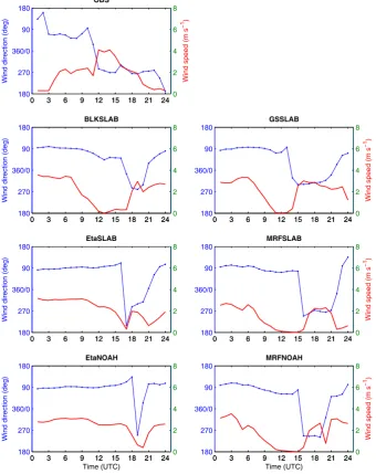
[image:12.595.126.468.67.496.2]

973 974 975

Fig. 7. Same as Fig. 2 but at Lejonet site.

On the other hand, comparing EtaSLAB with MRFSLAB, it is found that when coupled with the SLAB LSM, the Eta PBL produces stronger SB vertical circulation than MRF PBL, which is characterized by larger inland penetration dis-tance, larger U-component maximum, larger updraft veloc-ity maximum, and larger SBCI. The simulated downdraft ve-locity maxima by these two PBLs are comparable. In con-trast, when coupled with Noah LSM, the Eta PBL also pre-dicts a similar inland penetration distance to the MRF PBL, a larger U-component maximum than the MRF PBL, but pre-dicts smaller updraft and downdraft velocity maxima than the MRF PBL. As a result, the simulated SBCI index by the Eta PBL is somewhat weaker than that by the MRF PBL. The BLKSLAB (Blackadar PBL) produces a larger SBCI relative

(13)

44

0 3 6 9 12 15 18 21 24

180 270 360/0 90 180

0 3 6 9 12 15 18 21 240

2 4 6 8

BLKSLAB

0 3 6 9 12 15 18 21 24

180 270 360/0 90 180

0 3 6 9 12 15 18 21 240

2 4 6 8

Wind speed (m s

−

1)

GSSLAB

0 3 6 9 12 15 18 21 24

180 270 360/0 90 180

0 3 6 9 12 15 18 21 240

2 4 6 8

EtaSLAB

0 3 6 9 12 15 18 21 24

180 270 360/0 90 180

0 3 6 9 12 15 18 21 240

2 4 6 8

Wind speed (m s

−

1)

MRFSLAB

0 3 6 9 12 15 18 21 24

180 270 360/0 90 180

0 3 6 9 12 15 18 21 240

2 4 6 8

Time (UTC)

EtaNOAH

0 3 6 9 12 15 18 21 24

180 270 360/0 90 180

0 3 6 9 12 15 18 21 240

2 4 6 8

Wind speed (m s

−

1)

Time (UTC)

MRFNOAH

0 3 6 9 12 15 18 21 24

180 270 360/0 90 180

0 3 6 9 12 15 18 21 240

2 4 6 8

Wind speed (m s

−

1)

OBS

976 977

Fig. 8 978

[image:13.595.129.465.65.500.2]

979 980 981 982 983

Fig. 8. Same as Fig. 2 but at Tagene site.

schemes do not simulate such circulations very much. This is mainly devoted to impacts of boundary layer and land sur-face parameterizations implemented in the model.

The above results indicate that the impacts from the com-bination of PBL and LSM parameterizations on the simula-tions of SB vertical circulation are significant. The reasons behind these differences resulting from using different com-binations of PBL and LSM parameterization schemes need to be further investigated in the future. One of the interest-ing ways is to apply sea breeze scalinterest-ing (Steyn, 1998, 2003; Wichink Kruit et al., 2004; Drobinski et al., 2006) to the simulated results, because the recent studies have shown that the sea-breeze speed scale is controlled by surface heat flux whereas the depth scale is controlled by stability (Wichink

Kruit et al., 2004; Porson et al., 2007a, b). Such analyses would assist in highlighting the deficiencies in PBL and/or LSM schemes, and determine the level of coupling between the land surface and the atmosphere.

6 Summary and conclusions

(14)

[image:14.595.85.505.69.623.2]

984 985

Fig. 9

986

987 988 989 990 991 992 993

Fig. 9. Vertical cross section of simulated wind vector (U- andW-component) and potential temperature along 57.72◦N (cf. Fig. 1b) with

different experiments at 15:00 UTC 8 May 2001. TheW-component has been multiplied by a factor of 50. Contour interval for potential

temperature is 2 K. Number 0 on abscissa (X-axis) indicates coastline. Positive number on X-axis is onshore (inland) distance from the coastline (in kilometers), while negative number is offshore distance from coastline.

[image:14.595.309.508.69.621.2]

(15)

[image:15.595.72.523.99.269.2]

Table 5. Simulated sea breeze (SB) circulation characteristics with different experiments, which are based on vertical cross section ofUand

Wcomponents along 57.72◦N at 15:00 UTC 8 May 2001.

SB circulation characteristicsa Experiment

c

BS GS ES MS EN MN

Inland penetration distance (km) 8 20 12 10 8 8

SB depth maximum (m) 421 500 343 421 343 421

U-component maximum Magnitude (UMAX)(m s−1) 4.9 6.7 5.6 4.5 5.7 4.5

At distance from coastline (km) −2 14 6 −2 −2 −2

At height (m a.g.l.) 38 142 85 38 38 38

Updraft velocity maximum Magnitude (W+)(cm s−1) 42.7 67.6 37.1 26.7 31.6 39.7

At distance from coastline (km) 8 18 10 10 8 8

At height (m a.g.l.) 539 539 539 619 539 699

Downdraft velocity maximum Magnitude (W−)(cm s−1) −13.3 −20.0 −12.5 −14.3 −6.3 −14.6

At distance from coastline (km) 6 16 8 4 0 2

At height (m a.g.l.) 1109 1647 1450 1109 1278 1109

SB circulation intensityb(m2s−2) 2.744 5.869 2.778 1.854 2.160 2.444

a_{Inland penetration distance is defined as the distance at which the magnitude of} _U_{-component at the lowest model level (10 m a.g.l.)}

becomes less than 0.0 m s−1from positive to negative; SB depth maximum is defined as the maximum depth of a consistently positive

U-component near the coastline;UMAXis defined as the maximum positive U-component indicating SB (onshore);W+is defined as the

maximumW-component (positive) ahead of the SB front, andW−is defined as the minimumW-component (negative) behind the SB front

(cf. Miao et al., 2003).

b_{SB circulation intensity (SBCI) is defined as: SBCI=}_U

MAX×(W+−W−).

c_{Refer to Table 1 for abbreviations of experiments.}

vertical resolutions are used, and 3) the timing and strength of SB circulation is evaluated and intercompared.

The experiments aim at the simulations of a typical SB case (8 May 2001) over the Swedish west coast. The sim-ulated 10-m winds are compared among different combina-tions of PBL and LSM schemes, and compared against the observed near-surface wind from the G ¨OTE2001 field cam-paign. The focus is on SB timing and wind direction. The main conclusions are:

– All combinations of PBL and LSM schemes can re-produce the observed SB at the coastal sites (Kan-otföreningen, Risholmen) and the near-coastal site (Järnbrott) to a larger extent, but some differences in the simulated SB onset, life span and strength do exist. All experiments predict a delayed SB. BLKSLAB, MRFS-LAB and MRFNOAH show better performance in pre-dicting SB onset and life span at the two coastal sites. BLKSLAB and GSSLAB perform better at the Järnbrott site, and EtaSLAB, MRFSLAB and MRFNOAH ex-hibit similar performance at this site. As a whole, BLK-SLAB is shown to perform the best among the six ex-amined combinations of the PBL and LSM schemes in reproducing the SB onset and life span at the coastal or near-coastal sites.

– GSSLAB, EtaSLAB and MRFSLAB predict SB inland penetration reasonably well compared to the observed

SB, while BLKSLAB, EtaNOAH and MRFNOAH pre-dict shorter inland distance penetration distance. – The simulated SB characteristics, especially the

in-tensity of the SB vertical circulation, are highly vari-able. GSSLAB predicts the strongest SB circula-tion, and BLKSLAB predicts a similar intensity of SB circulation to EtaSLAB and MRFNOAH. MRFSLAB and EtaSLAB predict somewhat weaker SB circula-tion. There is an evident difference between SLAB and Noah LSMs in simulated SB circulation intensity (SBCI) (EtaSLAB versus EtaNOAH, and MRFSLAB versus MRFNOAH).

In summary, choosing different combinations of PBL and LSM parameterization schemes in MM5 as applied to SB simulations exhibits different model performance in simu-lated SB timing, inland penetration distance, and circulation intensity. These differences are not only due to combination (coupling) of the different PBL schemes with the same LSM scheme (e.g., BLKSLAB, GSSLAB, EtaSLAB and MRFS-LAB for SMRFS-LAB LSM; EtaNOAH and MRFNOAH for Noah LSM), but also due to combination of different LSM schemes with the same PBL scheme (e.g., EtaSLAB and EtaNOAH for Eta PBL; MRFSLAB and MRFNOAH for MRF PBL).

(16)

2318 J.-F. Miao et al.: Impacts of boundary layer turbulence and land surface process parameterizations LSM scheme does not imply better results than with the

sim-pler SLAB LSM scheme.

At last, it is necessary to point out that: 1) more case studies of SB under different large-scale forcing conditions and/or over different geographical regions (e.g., complex ter-rain) should be done to generalize our findings, and 2) appli-cation of sea breeze scaling to the simulated results could significantly improve our understanding of the differences caused by using different combination of PBL and LSM pa-rameterization schemes in the SB simulations.

Acknowledgements. The study was funded by Adlerbertska Re-search Foundation (Adlerbertska Forskingsstiftelsen, Sweden) through the project Sea Breeze Study over the Swedish west coast by using Mesoscale Meteorological Model: Soil-Vegetation-Atmosphere Interaction to Junfeng Miao. Additional financial sup-port to Junfeng Miao for this research is provided by the Cana-dian Foundation for Climate and Atmospheric Sciences (CFCAS) through a sub-project on Sea Breeze and Fog Modelling within Interdisciplinary Marine Environmental Prediction in the Atlantic Coastal Region (“The Lunenburg Bay Project”). The authors are greatly thankful to Katarina Borne (University College of Bor˚as, Sweden) and Jesper Lindgren (Environment Administration of the

City of Gothenburg, Sweden) for the G ¨OTE2001 data support.

Deliang Chen’s contribution is Contribution Number 26 from TEL-LUS, the Centre for Earth Systems Science at University of Gothen-burg. Moreover, this study is also supported by the Scientific Re-search Fund of Nanjing University of Information Science and Technology (NUIST) and the Dean’s Fund of College of Atmo-spheric Sciences of NUIST.

Topical Editor F. D’Andrea thanks two anonymous referees for their help in evaluating this paper.

References

Abbs, D. and Physick, W.: Sea-breeze observations and modeling: A review, Aust. Meteor. Mag., 41, 7–19, 1992.

Akylas, E., Kotroni. V., and Lagouvardos, K.: Sensitivity of high-resolution operational weather forecasts to the choice of the plan-etary boundary layer scheme, Atmos. Res., 84, 49–57, 2007.

Angevine, W. M., Tjernstr¨om, M., and ˇZagar, M.: Modeling of the

coastal boundary layer and pollutant transport in New England, J. Appl. Meteor. Climatol., 45, 137–154, 2006.

Augustin, P., Delbarre, H., Lohou, F., Campistron, B., Puygrenier, V., Cachier, H., and Lombardo, T.: Investigation of local mete-orological events and their relationship with ozone and aerosols during an ESCOMPTE photochemical episode, Ann. Geophys., 24, 2809–2822, 2006,

http://www.ann-geophys.net/24/2809/2006/.

Berg, L. K. and Zhong, S. Y.: Sensitivity of MM5-simulated bound-ary layer characteristics to turbulence parameterizations, J. Appl. Meteorol., 44, 1467–1483, 2005.

B´elair, S. and Mailhot, J.: Impact of horizontal resolution on the numerical simulation of a midlatitude squall line: Implicit ver-sus explicit condensation, Mon. Weather Rev., 129, 2362–2376, 2001.

Bianco, L., Tomassetti, B., Coppola, E., Fracassi, A., Verdecchia, M., and Visconti, G.: Thermally driven circulation in a region of

complex topography: comparison of wind-profiling radar mea-surements and MM5 numerical predictions, Ann. Geophys., 24, 1537–1549, 2006,

Blackadar, A. K.: Modeling the nocturnal boundary layer. Preprints, Third Symposium on Atmospheric Turbulence, Diffusion and Air Quality, Raleigh, NC, American Meteorological Society, 46– 49, 1976.

Blackadar, A. K.: High resolution models of the planetary boundary layer, in: Advances in Environmental Science and Engineering, edited by: Pfafflin, J. and Ziegler, E., vol. 1, no. 1, Gordon and Breach Publishers, Newark, 50–85, 1979.

Borne, K., Chen, D., and Nunez, M.: A method for finding sea breeze days under stable synoptic conditions and its application to the Swedish west coast, Int. J. Climatol., 18, 901–914, 1998. Borne, K., Chen, D., Miao, J.-F., Achberger, C., Lindgren, J.,

Hallquist, M., Pettersson, J., Haeger Eugensson, M., Wyser, K., Eliasson, I., and Langner, J.: Data report on measurements of meteorological- and air pollution variables during the

cam-paign G ¨OTE-2001, Research Report C67, Earth Sciences Centre,

G¨oteborg University, G¨oteborg, Sweden, 28 pp., 2005.

Bossioli, E., Tombrou, M., Dandou, A., Athanasopoulou, E., and Varotsos, K. V.: The role of planetary boundary-layer parameter-izations in the air quality of an urban area with complex topog-raphy, Bound.-Lay. Meteorol., 131, 53–72, 2009.

Braun, S. A. and Tao, W. K.: Sensitivity of high-resolution sim-ulations of Hurricane Bob (1991) to planetary boundary layer parameterizations, Mon. Weather Rev., 128, 3941–3961, 2000. Bright, D. R. and Mullen, S. L.: The sensitivity of the

numeri-cal simulation of the southwest monsoon boundary layer to the choice of PBL turbulence parameterization in MM5, Wea. Fore-cast., 17, 99–114, 2002.

Chen, F. and Dudhia, J.: Coupling an advanced land surface-hydrology model with the Penn State-NCAR MM5 modeling system. Part I: Model implementation and sensitivity, Mon. Weather Rev., 129, 569–585, 2001a.

Chen, F. and Dudhia, J.: Coupling an advanced land surface-hydrology model with the Penn State-NCAR MM5 modeling system. Part II: Preliminary model validation, Mon. Weather Rev., 129, 587–604, 2001b.

Colby Jr., F. P.: Simulation of the New England sea breeze: The effect of grid spacing, Wea. Forecast., 19, 277–285, 2004. Dandou, A., Tombrou, M., and Soulakellis, N.: The influence of the

City of Athens on the evolution of the sea-breeze front, Bound.-Lay. Meteorol., 131, 35–51, 2009a.

Dandou, A., Tombrou, M., Sch¨afer, K., Emeis, S., Protonotariou, A. P., Bossioli, E., Soulakellis, N., and Suppan, P.: A Compar-ison between modelled and measured mixing-layer height over Munich, Bound.-Lay. Meteorol., 131, 425–440, 2009b. Ding, A. J., Wang, T., Zhao, M., Wang, T. J., and Li, Z. K.:

Simula-tion of sea-land breezes and a discussion of their implicaSimula-tions on the transport of air pollution during a multi-day ozone episode in the Pearl River Delta of China, Atmos. Environ., 38, 6737–6750, 2004.

Drobinski, P., Bastin, S., Dabas, A., Delville, P., and Reitebuch, O.: Variability of three-dimensional sea breeze structure in southern France: observations and evaluation of empirical scaling laws, Ann. Geophys., 24, 1783–1799, 2006,

(17)

Dudhia, J.: Numerical study of convection observed during the Winter Monsoon Experiment using a mesoscale two-dimensional model, J. Atmos. Sci., 46, 3077–3107, 1989.

Dudhia, J.: A multi-layer soil temperature model for MM5,

Reprints, Sixth Annual PSU/NCAR Mesoscale Model Users’ Workshop, Boulder, CO, NCAR, 49–50, 1996.

Freitas, E. D., Rozoff, C. M., Cotton, W. R., and Silva Dias, P. L.: Interactions of an urban heat island and sea-breeze circulations during winter over the metropolitan area of S˜ao Paulo, Brazil, Bound.-Lay. Meteorol., 122, 43–65, 2007.

Furberg, M., Steyn, D. G., and Baldi, M.: The climatology of sea breezes on Sardinia, Int. J. Climatol., 22, 917–932, 2002. Grell, G. A., Dudhia, J., and Stauffer, D. R.: A description of the

fifth-generation Penne State/NCAR Mesoscale Model (MM5), NCAR Technical Note, NCAR/TN-398+STR, National Center for Atmospheric Research, Boulder, CO, 122 pp., 1995. Gronas, S. and Sandvik, A. D.: Numerical simulations of sea and

land breezes at high latitudes, Tellus, 50A, 468–489, 1998. Gustavsson, T., Lindqvist, S., Borne, K., and Bogren, J.: A study

of sea and land breezes in an Archipelago on the west coast of Sweden, Int. J. Climatol., 15, 785–800, 1995.

Han, Z., Ueda, H., and An, J.: Evaluation and intercomparison of meteorological predictions by five MM5-PBL parameterizations in combination with three land-surface models, Atmos. Environ., 42, 233–249, 2008.

Hong, S. Y. and Pan, H. L.: Nonlocal boundary layer vertical diffu-sion in a medium-range forecast model, Mon. Weather Rev., 124, 2322–2339, 1996.

Janji´c, Z. I.: The step-mountain coordinate: Physical package, Mon. Weather Rev., 118, 1429–1443, 1990.

Janji´c, Z. I.: The step-mountain Eta coordinate model: Further de-velopments of the convection, viscous sublayer, and turbulence closure schemes, Mon. Weather Rev., 122, 927–945, 1994. Kain, J. S.: The Kain-Fritsch convective parameterization: An

up-date, J. Appl. Meteorol., 43, 170–181, 2004.

Lo, J. C. F., Lau, A. K. H., Chen, F., Fung, J. C. H., and Leung, K. K. M.: Urban modification in a mesoscale model and the effects on the local circulation in the Pearl River Delta Region, J. Appl. Meteor. Climatol., 46, 457–476, 2007.

Malda, D., Vil`a-Guerau de Arellano, J., van den Berg, W. D., and Zuurendonk, I. W.: The role of atmospheric boundary layer-surface interactions on the development of coastal fronts, Ann. Geophys., 25, 341–360, 2007,

Manabe, S.: Climate and the ocean circulation – I. The atmo-spheric circulation and the hydrology of the Earth’s surface, Mon. Weather Rev., 97, 739–774, 1969.

Mao, Q., Gautney, L. L., Cook, T. M., Jacobs, M. E., Smith, S. N., and Kelsoe, J. J.: Numerical experiments on MM5-CMAQ sensitivity to various PBL schemes, Atmos. Environ., 40, 3092– 3110, 2006.

Martilli, A.: A two-dimensional numerical study of the impact of a city on atmospheric circulation and pollutant dispersion in a coastal environment, Bound.-Lay. Meteorol., 108, 91–119, 2003. Miao, J.-F.: Meteorological modelling in coastal areas – Local cli-mate and air quality, Ph.D. thesis, A107, Earth Sciences Centre, Göteborg University, Göteborg, Sweden, 190 pp., 2006. Miao, J.-F., Kroon, L. J. M., Vilà-Guerau de Arellano, J., and

Holt-slag, A. A. M.: Impacts of topography and land degradation on

the sea breeze over eastern Spain, Meteorol. Atmos. Phys., 84, 157–170, 2003.

Miao, J.-F., Chen, D., and Wyser, K.: Modelling subgrid scale

dry deposition velocity of O3over the Swedish west coast with

MM5-PX model, Atmos. Environ., 40, 415–429, 2006. Miao, J.-F., Chen, D., and Borne, K.: Evaluation and

compari-son of Noah and Pleim-Xiu land surface models in MM5

us-ing G ¨OTE2001 data: Spatial and temporal variations in

near-surface air temperature, J. Appl. Meteor. Climatol., 46, 1587– 1605, 2007.

Miao, J.-F., Chen, D., Wyser, K., Borne, K., Lindgren, J., Svensson, M. K., Thorsson, S., Achberger, C., and Almkvist, E.: Evaluation of MM5 mesoscale model at local scale for air quality applica-tions over the Swedish west coast: Influence of PBL and LSM parameterizations, Meteorol. Atmos. Phys., 99, 77–103, 2008. Miller, S. T. K., Keim, B. D., Talbot, R. W., and Mao, H.: Sea

breeze: Structure, forecasting, and impacts, Rev. Geophys., 41(3), 1011, doi:10.1029/2003RG000124, 2003.

Mlawer, E. J., Taubman, S. J., Brown, P. D., Iacono, M. J., and Clough, S. A.: Radiative transfer for inhomogeneous atmo-spheres: RRTM, a validated correlated-K model for the long-wave, J. Geophys. Res., 102(D14), 16663–16682, 1997. Oh, I. B., Kim, Y. K., Lee, H. W., and Kim, C. H.: An observational

and numerical study of the effects of the late sea breeze on ozone distributions in the Busan metropolitan area, Korea, Atmos. En-viron., 40, 1284–1298, 2006.

Ohashi, Y. and Kida, H.: Local circulations developed in the vicin-ity of both coastal and inland urban areas: A numerical study with a mesoscale atmospheric model, J. Appl. Meteorol., 41, 30– 45, 2002.

Orli´c, M., Penzar, B., and Penzar, I.: Adriatic sea and land breezes: Clockwise versus anticlockwise rotation, J. Appl. Meteorol., 27, 675–679, 1988.

P´erez, C., Jim´enez, P., Jorba, O., Sicard, M., and Baldasano, J. M.: Influence of the PBL scheme on high-resolution photochemical simulations in an urban coastal area over the Western Mediter-ranean, Atmos. Environ., 40, 5274–5297, 2006.

Pleim, J. E.: A combined local and nonlocal closure model for the atmospheric boundary layer. Part II: application and evaluation in a mesoscale meteorological model, J. Appl. Meteorol., 46, 1396– 1409, 2007.

Porson, A., Steyn, D. G., and Schayes, G.: Sea-breeze scaling from numerical model simulations, Part I: Pure sea breezes, Bound.-Lay. Meteorol., 122, 17–29, 2007a.

Porson, A., Steyn, D. G., and Schayes, G.: Sea-breeze scaling from numerical model simulations, part II: Interaction between the sea breeze and slope flows, Bound.-Lay. Meteorol., 122, 31–41, 2007b.

Prezerakos, N. G.: Characteristics of the sea breeze in Attica, Greece, Bound.-Lay. Meteorol., 36, 245–266, 1986.

Prtenjak, M. T. and Grisogono, B.: Idealised numerical simulations of diurnal sea breeze characteristics over a step change in rough-ness, Meteorol. Z., 11, 345–360, 2002.

Prtenjak, M. T. and Grisogono, B.: Sea/land breeze climatological characteristics along the northern Croatian Adriatic coast, Theor. Appl. Climatol., 90, 201–215, 2007.

Seaman, N. L.: Meteorological modeling for air-quality assess-ments, Atmos. Environ., 34, 2231–2259, 2000.

(18)

nu-2320 J.-F. Miao et al.: Impacts of boundary layer turbulence and land surface process parameterizations

merical predictions of boundary layer structure during the Lake Michigan ozone study, J. Appl. Meteorol., 39, 412–426, 2000. Simpson, J. E.: Sea breeze and local winds. Cambridge University

Press, UK, 234 pp., 1994.

Simpson, J. E.: Diurnal changes in sea-breeze direction, J. Appl. Meteorol., 35, 1166–1169, 1996.

Srinivas, C. V., Venkatesan, R., and Bagavath Singh, A.: Sensitivity of mesoscale simulations of land-sea breeze to boundary layer turbulence parameterization, Atmos. Environ., 41, 2534–2548, 2007.

Steyn, D. G.: Scaling the vertical structure of sea breezes, Bound.-Lay. Meteorol., 86, 505–524, 1998.

Steyn, D. G.: Scaling the vertical structure of sea breezes revised. Bound.-Lay. Meteorol., 107, 177–188, 2003.

Thomsen, G. L. and Smith, R. K.: The importance of the boundary layer parameterization in the prediction of low-level convergence lines, Mon. Weather Rev., 136, 2173–2185, 2008.

Tombrou, M., Dandou, A., Helmis, C., Akylas, E., Angelopoulos, G., Flocas, H., Assimakopoulos, V., and Soulakellis, N.: Model evaluation of the atmospheric boundary layer and mixed-layer evolution, Bound.-Lay. Meteorol., 124, 61–79, 2007.

Wichink Kruit, R. J., Holtslag, A. A. M., and Tijm, A. B. C.: Scaling of the sea-breeze strength with observations in the Netherlands, Bound.-Lay. Meteorol., 112, 369–380, 2004.

Wisse, J. S. P. and Vil`a-Guerau de Arellano, J.: Analysis of the role of the planetary boundary layer schemes during a severe convec-tive storm, Ann. Geophys., 22, 1861–1874, 2004,

Yoshikado, H.: Numerical study of the daytime urban effect and its interaction with the sea breeze, J. Appl. Meteorol., 31, 1146– 1164, 1992.

Z¨angl, G., Gohm, A., and Obleitner, F.: The impact of the PBL scheme and the vertical distribution of model layers on simu-lations of Alpine foehn, Meteorol. Atmos. Phys., 99, 105–128, 2008.

Zhang, D. L. and Anthes, R. A.: A high-resolution model of the planetary boundary layer – Sensitivity tests and compar-isons with SESAME-79 data, J. Appl. Meteorol., 21, 1594–1609, 1982.

Zhang, D. L. and Zheng, W. Z.: Diurnal cycles of surface winds and temperatures as simulated by five boundary layer parameteriza-tions, J. Appl. Meteorol., 43, 157–169, 2004.

Zhong, S. Y. and Takle, E. S.: The effects of large-scale winds on the sea–land-breeze circulations in an area of complex coastal heating, J. Appl. Meteorol., 32, 1181–1195, 1993.

Zhong, S. Y., In, H. J., Bian, X. D., Charney, J., Heilman, W., and Potter, B.: Evaluation of real-time high-resolution MM5 predic-tions over the Great Lakes region, Wea. Forecast., 20, 63–81, 2005.

Zhong, S. Y., In, H. J., and Clements, C.: Impact of turbulence, land surface, and radiation parameterizations on simulated boundary layer properties in a coastal environment, J. Geophys. Res., 112, D13110, doi:10.1029/2006JD008274, 2007.