www.adv-radio-sci.net/8/251/2010/ doi:10.5194/ars-8-251-2010
© Author(s) 2010. CC Attribution 3.0 License.
Radio Science
Single snapshot DOA estimation
P. H¨acker and B. Yang
Chair of System Theory and Signal Processing, Universit¨at Stuttgart, Pfaffenwaldring 47, 70550 Stuttgart, Germany
Abstract. In array signal processing, direction of arrival (DOA) estimation has been studied for decades. Many algo-rithms have been proposed and their performance has been studied thoroughly. Yet, most of these works are focused on the asymptotic case of a large number of snapshots. In automotive radar applications like driver assistance systems, however, only a small number of snapshots of the radar sen-sor array or, in the worst case, a single snapshot is available for DOA estimation.
In this paper, we investigate and compare different DOA estimators with respect to their single snapshot performance. The main focus is on the estimation accuracy and the angular resolution in multi-target scenarios including difficult situ-ations like correlated targets and large target power differ-ences. We will show that some algorithms lose their ability to resolve targets or do not work properly at all. Other so-phisticated algorithms do not show a superior performance as expected. It turns out that the deterministic maximum likeli-hood estimator is a good choice under these hard conditions.
1 Introduction
A common problem in array signal processing is the estima-tion of the DOA ofMtargets usingNsensors. As within au-tomotive applications the elevation angels are less important, there areMangles (azimuth) to be estimated. Together with the distances, the angels determine the position of the rele-vant targets uniquely relative to the host vehicle. Using this information, the car can act in an intelligent way. Two exam-ples of such driver assistance systems are Adaptive Cruise Control (ACC) and initializing an emergency brake (Jurgen, 2006).
Classical radar systems measure their environment using a grid of distance and relative velocity cells. This represen-tation is sparse. The linear frequency modulated continuous wave (LFMCW) principle uses frequency sweeps (ramps) to
Correspondence to: P. H¨acker
get projections of this plane which is more efficient. Every ramp contains the targets at different frequencies, depend-ing on its slope. Usdepend-ing multiple ramps, the whole plane can be reconstructed (Reiher and Yang, 2009). However, targets with similar frequencies can only be separated by their DOA. The number of antennas and the number of snapshots are limited to get a cheap sensor. To still get acceptable results, the DOA estimator has to be as good as possible. There are many papers covering DOA algorithms using a huge amount of antennas, samples per antenna or a high SNR, respec-tively (Ottersten et al., 1992; Li et al., 1998; Xin and Sano, 2004; Viberg et al., 1991b; Lopes et al., 2003; Stoica and Sharman, 1990b; Gershman and Stoica, 1999), to make use of statistical asymptotic analysis. Yet, there are few papers which deal with the single snapshot case. There was a suc-cessful examination of the two classical ML algorithms (Rife and Boorstyn, 1974, 1976; Athley, 2005). However, to the knowledge of the authors, there is still no comparative study about which DOA algorithm to choose in the single snapshot case, which is what this paper is about.
There are several reasons, why a single snapshot DOA es-timation is attractive in automotive radar systems:
– LFMCW ramps are designed for different ranges. In general, not all ramps are available for all distance-velocity-combinations.
– Some snapshots may be distorted by close frequency in-terferer and thus should not be used for angle estima-tion.
– Some snapshots are superpositioned by clutter. These snapshots should be avoided as well.
– The speed of reaction is enhanced by using snapshots immediately after measurement, instead of waiting for a large number of snapshots.
– The computation time is decreased as the single snap-shot case allows some additional simplifications in DOA estimation.
We shortly introduce the used notation in Sect. 2 and the signal models in Sect. 3. We then take a closer look on the DOA algorithms in Sect. 4, separate them into usable and non-usable algorithms with regard to the problem at hand. In Sect. 5, we use typical automotive scenarios to simulate the performance of the DOA algorithms and conclude our work in Sect. 6.
2 Notation
The following notations are used in this paper: Uppercase bold letters are matrices, lowercase bold letters are vectors, letters with a hat are estimations,(·)Tdenotes the transposi-tion,(·)H denotes the complex conjugate transposition,(·)† denotes the Moore-Penrose pseudo inverse, argmax
θ
(·) de-notes the θ maximizing the function, argmaxima
θ
M(·) de-notes theθof theMlargest local maxima, Tr(·)is the matrix trace operator,| · |is the matrix determinant and I is the iden-tity matrix.
3 Signal models
Two signal models are commonly used for DOA estima-tion (Krim and Viberg, 1996): the deterministic model and the stochastic model. In both models, the impinging sig-nals on the array are superpositioned by spatial and temporal white Gaussian noisen(t ). In typical automotive applica-tions, narrow band and far field conditions can be assumed to be valid. Furthermore, both signal models parametrize the sensor array and the targets’ DOA by the steering matrix A(θ)=(a(θ1),...,a(θM)). (1) a(θ )is the steering vector which can be seen as an angular transfer function. Using a uniform linear array (ULA) can re-duce the signal processing effort. In general, the array can be arbitrary. For the linear array used in this paper, the steering vector can be written as
a(θ )=ej2πy1sin(θ ),...,ej2πyNsin(θ )T (2)
using the sensor positionsynnormalized by the wavelength. θis defined as 0◦pointing to the front direction.
Lets(t )be the incoming waves after mixing to baseband, the sensor array signal to be processed is given by
x(t )=A(θ)s(t )+n(t ). (3) The source signalss(t )can be deterministic or a Gaussian random process, depending on the chosen signal model. Us-ing an LFMCW radar (Schoor and Yang, 2007) most of the
targets are separated by their distance and relative velocity. The DOA estimations separate only the remaining targets. This is why most often only one or two targets need to be estimated using a single snapshotx(t ).
The used array is a half wavelength minimum redundancy array (Moffet, 1968) consisting of four antennas (M=4) at the positionsy=(0,0.5,2,3)T normalized by the wave-length. As the distance between the first two antennas is half of the wavelength, the uniqueness of the DOA estima-tion is guaranteed. The missing redundancy leads to a high positional variance (Athley, 2005) and thus to an improved accuracy of the single target estimation compared to more conservative four antenna arrays.
4 DOA algorithms
The following DOA algorithms are studied in this paper: Bartlett beamformer, Multiple Signal Classification (MU-SIC), Deterministic Maximum Likelihood (DML), Stochas-tic Maximum Likelihood (SML) and Weighted Subspace Fit-ting (WSF).
Since the array assumptions shift invariance, rotational in-variance, special structure and the invertability of the sample correlation matrix are not fullfilled, many DOA estimation algorithms like estimators using decorrelation principles (Pil-lai and Kwon, 1989), Capon’s beamformer (Capon, 1969), ESPRIT (Paulraj et al., 1985), Root-MUSIC (Barabell, 1983), MUD (Swindlehurst, 1991), IQML (Swindlehurst, 1991), MODE (Stoica and Sharman, 1990a) or MODEX (Gershman and Stoica, 1999) do not work and are thus not considered in this paper.
4.1 Bartlett beamformer
Bartlett’s beamformer can be written, using the sample cor-relation matrix
ˆ
R=x(t )x(t )H (4)
as
ˆ
θBartlett=argmaxima
θ M
a(θ )HRˆa(θ )
a(θ )Ha(θ )
!
. (5)
The Bartlett beamformer maximizes the angular spectrum in Eq. (5) and returns the position of theMlargest maxima as the estimates for the DOAs of theMtargets. An example of a beamformer spectrum is given in Fig. 1. In this scenario two 40 dB targets are at 0◦and 60◦. Since only a single snapshot is used, the Bartlett beamformer does not show maxima at the correct DOAs. The largest maximum appears even at a DOA where no target exists.
4.2 MUSIC
To get the MUSIC function, an eigenvalue decomposition of
ˆ
−90 −60 −30 0 30 60 90
steering angle in degree
Fig. 1. Bartlett beamformer spectrum for two targets.
−90 −60 −30 0 30 60 90
steering angle in degree
Fig. 2. MUSIC function for two targets.
to theN−Mweakest eigenvalues in the noise subspace ma-trix9ˆnoise, the MUSIC estimator is given by (Schmidt, 1979)
ˆ
θMUSIC=argmaxima
θ M
a(θ )Ha(θ )
a(θ )H9ˆ noise9ˆ
H noisea(θ )
!
. (6)
The MUSIC function is given in Fig. 2 using the same sce-nario and the same snapshot as before. MUSIC detects a non-existing target between the two real targets and it does not indicate the existence of two targets. As there is only one snapshot, the signal subspace is built up of only one eigen-vector, which leads to the averaged target.
4.3 DML
Using the deterministic signal model, the DML approach is
ˆ
θDML=argmax
θ
Tr5A(θ)Rˆ (7)
using the projection matrix onto the column space of A(θ)
5A(θ)=A(θ)A(θ)† (8)
and the pseudo inverse of A(θ) A(θ)†=
A(θ)HA(θ) −1
A(θ)H. (9)
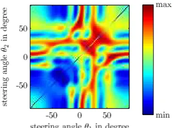
Once again, a typical DML function is drawn in Fig. 3 for the same situation.θ=(θ1,θ2)Tis now a two-element DOA
Fig. 3. DML function for two targets.
vector. While the Bartlett beamformer and MUSIC perform an one-dimensional search to estimateθ1andθ2of two
tar-gets, DML performs a two-dimensional search to estimate θ1 andθ2simultaneously. Note the symmetry of the figure
along its diagonal. It stems from the commutativity of the two targets, as the target numbering is arbitrary. We see from Fig. 3 that the maximum of the DML function is reached at either(0◦,60◦)or(60◦,0◦).
Besides its interpretation of the maximization of a likeli-hood function, Eq. (7) can be seen as maximizing the power of the input signals projected onto the model signal subspace.
4.4 SML
According to (Jaffer, 1988), the SML algorithm can be writ-ten as
ˆ
θSML=argmax
θ
−log A(θ)
OP(θ)A(θ)H+ ˆσ2(θ)I
(10) using the signal projection
OP(θ)=A(θ)†Rˆ− ˆσ2(θ)I A(θ)†
H
(11) together with the DOA dependent noise power estimation
ˆ
σ2(θ)= 1
N−MTr
5⊥A(θ)Rˆ (12)
and the orthogonal projection matrix
5⊥A(θ)=I−5A(θ). (13)
Fig. 4. SML function for two targets.
4.5 WSF
One approach to combine the ideas from ML and subspace based estimators is to use the signal subspace as the source of a projection into the model space, which is known as the WSF algorithm (Viberg et al., 1991a; Haykin et al., 1993). Analog to MUSIC, the eigenvalue decomposition is needed, but WSF uses the strongest eigenvalues in a diagonal matrix
ˆ
3signaland the corresponding eigenvectors in the signal sub-space matrix9ˆ
signal. WSF can then be written as ˆ
θWSF=argmax
θ
Tr5A(θ)9ˆsignalW9ˆH signal
, (14)
where W is a weighting matrix to reduce the impact of the subspace swap (Johnson et al., 2008a,b) defined as
W=3ˆsignal−2σˆ2I+ ˆσ23ˆ−signal1 (15)
Instead of Eq. (12), an estimation forσˆ2 independent ofθ can be used to decrease the computational effort.
ˆ
σ2= 1
N−M N−M
X
k=1 ˆ
3noise,k. (16)
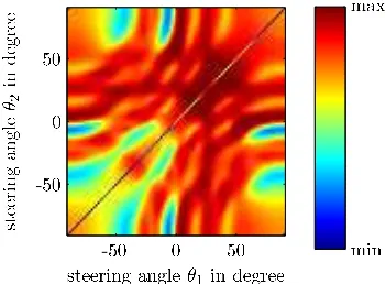
Note thatR is rank deficit in the two target case and the in-ˆ version of3ˆsignalis problematic. Nevertheless it can be done with a numerically robust algorithm leading to W with only one element differing from zero. Again, Fig. 5 shows the WSF function using the same snapshot as before. The func-tion has relatively broad maxima, which lead to higher vari-ances. Besides that, it is hard to differ the true DOAs from the single or close target case at around(30◦,30◦).
4.6 Complexity
When comparing the computational complexity of DOA al-gorithms, two aspects have to be distinguished. The first two algorithms do M one-dimensional optimizations, whereas
Fig. 5. WSF function for two targets.
the last three algorithms perform oneM-dimensional opti-mization, which is much more expensive for largeM. Fur-thermore, the effort for calculating a function value differs for different DOA algorithms. The order of the five con-sidered DOA algorithms in this paper is roughly sorted by increasing computation time.
5 Simulation results
To compare the performance of different DOA algorithms, we performed Monte Carlo simulations. The signals were generated according to the signal model and the optimiza-tions were done using a grid search followed by local opti-mizations.
The targets are estimated in the full angular range from
−90◦to 90◦and without any further postprocessing. The fol-lowing simulation results thus show the relative performance of different DOA estimators. The absolute performance can be improved by additional processing which is not subject of this paper.
In Fig. 6 we see that for one target in front direction and 1000 Monte Carlo trials, all algorithms behave the same for medium and large SNR values regarding their root mean squared error (RMSE). The estimators are close to the deter-ministic Cram´er-Rao Bound (CRB) which is included as an orientation. This is expected as it can be proofed, that MU-SIC, DML and WSF are the same as the Bartlett beamformer for a single snapshot and a single target. For very low SNR, the threshold region is reached and thus the distance between the estimators and the CRB rapidly increases (Athley, 2005). SML has a higher probability of outliers than the other al-gorithms and thus a higher RMSE. With only one snapshot, SML is significantly more sensitive to noise than the other DOA algorithms in this paper.
10 20 30 40 50 10−2
10−1
100
101
102
SNR in dB
RMSE
in
de
gree
Target at0◦, 1000 trials
Bartlett MUSIC DML SML WSF CRB
Fig. 6. DOA estimation of one target.
10 20 30 40 50 10−1
100
101
102
SNR in dB
A
v
erage
RMSE
in
de
gree
Uncorrelated targets at0◦and60◦, 300 trials
Bartlett MUSIC DML SML WSF
Fig. 7. DOA estimation of two widely spaced targets.
is the mean of 300 Monte Carlo trials, whereas the average after taking the root averages both targets. SML, MUSIC and the Bartlett beamformer are more or less useless. To-gether with their large errors, they lack an SNR dependency, which exposes a general modelling problem. WSF and DML behave better with DML being best.
In general, the average RMSE of both targets is dominated by outliers. So the estimation accuracy of most trials is much better than in the corresponding figures. There is only a frac-tion of trials which lead to large errors, but the fracfrac-tion de-pends on the DOA algorithm. Figures 7 and 8 show that the probability of outliers for DML is low.
It is interesting to note that widely spaced targets are not necessarily easier to resolve than close targets, when using a sparse array. This is because the envelope of the corre-lation of the non-sparse array is monotonically decreasing when starting at the main lobe. As the steering vectors are less similar, the estimation is less sensitive and thus more ac-curate. For general arrays there is no monotonic behaviour of the envelope of the correlation function and that is why Fig. 7 does not show better results than Fig. 8.
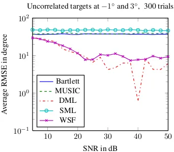
The situation in Fig. 9 seems more challenging than in
10 20 30 40 50
10−1
100
101
102
SNR in dB
A
v
erage
RMSE
in
de
gree
Uncorrelated targets at−1◦and3◦, 300 trials
Bartlett MUSIC DML SML WSF
Fig. 8. DOA estimation of two close targets.
10 20 30 40 50
10−1
100
101
102
SNR in dB
A
v
erage
RMSE
in
de
gree
Correlated targets at−1◦and3◦,10dB∆SNR, 300 trials
Bartlett MUSIC DML SML WSF
Fig. 9. DOA estimation of two differing correlated close targets.
Fig. 8. Two close targets at(−1◦,3◦)have an SNR differ-ence of 10 dB. One target has 5 dB less and the other one 5 dB more SNR than shown on the abscissa. The SNR differ-ence models radar cross section fluctuations when looking at the targets from different angles. Furthermore, the phase of the signals of the two targets are fully correlated, i.e. they are always the same, which can happen when crash barrier re-flections occur. This effect reduces the probability of outliers for DML and WSF and leads to an excellent DML perfor-mance. Further investigation is needed to give an exhaustive reason for that behaviour.
6 Conclusions
Acknowledgements. This research has partly been conducted with the support of the Robert Bosch Corporation, to which the authors would like to express their gratitude.
References
Athley, F.: Threshold Region Performance of Maximum Likelihood Direction of Arrival Estimators, IEEE Trans. on Signal Process-ing, 53, 1359–1373, 2005.
Barabell, A. J.: Improving the Resolution Performance of Eigenstructure-Based Direction Finding Algorithms, in: IEEE Proc. of Int. Conf. on Acoustics, Speech, and Signal Processing, 8, 336–339, 1983.
Capon, J.: High Resolution Frequency-Wavenumber Spectrum Analysis, IEEE Proc., 57, 1408–1418, 1969.
Gershman, A. B. and Stoica, P.: Mode with Extra-Roots (MODEX): A new DOA Estimation Algorithm with an Improved Threshold Performance, in: IEEE Proc. of Int. Conf. on Acoustics, Speech, and Signal Processing, 1999.
Haykin, S., Ho, T., Litva, J., McWhirter, J., Nehorai, A., and Nickel, U.: Radar Array Processing, Springer, 1 edn., 1993.
Jaffer, A. G.: Maximum Likelihood Direction Finding of Stochas-tic Sources: A Separable Solution, IEEE Proc. of Int. Conf. on Acoustics, Speech, and Signal Processing, 5, 2893–2896, 1988. Johnson, B. A., Abramovich, Y. I., and Mestre, X.: The Role
of Subspace Swap in Maximum Likelihood Estimation Per-formance Breakdown, IEEE Proc. of Int. Conf. on Acoustics, Speech, and Signal Processing, 2469–2472, 2008a.
Johnson, B. A., Abramovich, Y. I., and Mestre, X.: The Role of Subspace Swap in MUSIC Performance Breakdown, IEEE Proc. of Int. Conf. on Acoustics, Speech, and Signal Processing, 2473– 2476, 2008b.
Jurgen, R. K.: Adaptive Cruise Control, SAE International, 2006. Krim, H. and Viberg, M.: Two Decades of Array Signal Processing
Research, IEEE Signal Processing Magazine, 13, 67–94, 1996. Li, J., Stoica, P., and Liu, Z.-S.: Comparative Study of IQML and
MODE Direction-of-Arrival Estimators, IEEE Trans. on Signal Processing, 46, 149–160, 1998.
Lopes, A., Bonatti, I. S., Peres, P. L., and Alves, C. A.: Improving the MODEX Algorithm for Direction Estimation, ELSEVIER’s Signal Processing, 83, 2047–2051, 2003.
Moffet, A.: Minimum-Redundancy Linear Arrays, IEEE Trans. on Antennas and Propagation, 16, 172–175, 1968.
Ottersten, B., Viberg, M., and Kailath, T.: Analysis of Subspace Fitting and ML Techniques for Parameter Estimation from Sen-sor Array Data, IEEE Trans. on Signal Processing, 40, 590–600, 1992.
Paulraj, A., Roy, R., and Kailath, T.: Estimation of Signal Param-eters via Rotational Invariance Techniques – ESPRIT, in: Proc. of Asilomar Conf. on Circuits, Systems and Computers, 83–89, 1985.
Pillai, S. and Kwon, B.: Forward/Backward Spatial Smoothing Techniques for Coherent Signal Identification, IEEE Trans. on Acoustics, Speech, and Signal Processing, 37, 8–15, 1989. Reiher, M. and Yang, B.: Optimal Modulation Design in Linear
FMCW Radar Concerning Mismatch Probability, in: Proc. of Intern. Radar Symposium (IRS), 2009.
Rife, D. C. and Boorstyn, R. R.: Single-Tone Parameter Estimation from Discrete-Time Observations, IEEE Trans. on Information Theory, 20, 591–598, 1974.
Rife, D. C. and Boorstyn, R. R.: Multiple Tone Parameter Estima-tion from Discrete-Time ObservaEstima-tions, The Bell System Techni-cal Journal, 55, 1389–1411, 1976.
Schmidt, R. O.: Multiple Emitter Location and Signal Parameter Estimation, in: Proc. RADC Spectrum Estimation Workshop, 34, 243–258, 1979.
Schoor, M. and Yang, B.: High-Resolution Angle Estimation for an Automotive FMCW Radar Sensor, in: Proc. of Intern. Radar Symposium (IRS), Cologne, Germany, 2007.
Stoica, P. and Sharman, K.: Novel Eigenanalysis Method for Direc-tion EstimaDirec-tion, Radar and Signal Processing, IEE Proc. F, 137, 19–26, 1990a.
Stoica, P. and Sharman, K. C.: Maximum Likelihood Methods for Direction-of-Arrival Estimation, IEEE Trans. on Acoustics, Speech, and Signal Processing, 38, 1132–1143, 1990b. Swindlehurst, A.: Fast Updating of Maximum Likelihood Direction
of Arrival Estimates, in: Asilomar Conf. on Signals, Systems and Computers, 1, 302–306, 1991.
Viberg, M., Ottersten, B., and Kailath, T.: Detection and Estimation in Sensor Arrays Using Weighted Subspace Fitting, IEEE Trans. on Signal Processing, 39, 2436–2449, 1991a.
Viberg, M., Ottersten, B., and Nehorai, A.: Estimation Accuracy of Maximum Likelihood Direction Finding Using Large Arrays, Signals, Systems and Computers, 928–932, 1991b.