Proper Generalized Decomposition computational methods on a benchmark problem: introducing a new strategy based on Constitutive Relation Error minimization

Proper Generalized Decomposition

computational methods on a benchmark

problem: introducing a new strategy based

on Constitutive Relation Error minimization

Pierre‑Eric Allier

_{, Ludovic Chamoin and Pierre Ladevèze}

Notations

All continuous fields or spaces are in classical format u, while Finite Element approxima-tions fields uh benefit of an h index. Discretized terms, usually represented by vectors of nodal values, are bolded u and matrices are in uppercase and double-struck U.

Background

Nowadays, numerical simulations constitute a common tool in science and engineering activities. It is especially used for prediction and decision making, or simply for a bet-ter understanding of physical phenomena. However, in order to give an accurate repre-sentation of the real world, a large set of parameters and nonlinearities may need to be introduced in the mathematical models involved in the simulation, leading to important and often overwhelming computational effort. This results in a huge number of degrees of freedom, a drawback for such complex models, so that they cannot be tackled with classical brute force methods. Therefore, alternative numerical approaches are required, such as model reduction methods. These methods exploit the fact that the response of complex models can often be approximated with a reasonable accuracy by the response of a surrogate model, seen as the projection of the initial one on a lower dimensional

Abstract

First, the effectivity of classical Proper Generalized Decomposition (PGD) computational methods is analyzed on a one dimensional transient diffusion benchmark problem, with a moving load. Classical PGD methods refer to Galerkin, Petrov–Galerkin and Mini‑ mum Residual formulations. A new and promising PGD computational method based on the Constitutive Relation Error concept is then proposed and provides an improved, immediate and robust reduction error estimation. All those methods are compared to a reference Singular Value Decomposition reduced solution using the energy norm. Eventually, the variable separation assumption itself (here time and space) is analyzed with respect to the loading velocity.

Keywords: Model Reduction, Proper Generalized Decomposition (PGD), Separation of variables, Constitutive Relation Error (CRE)

Open Access

© 2015 Allier et al. This article is distributed under the terms of the Creative Commons Attribution 4.0 International License (http:// creativecommons.org/licenses/by/4.0/), which permits unrestricted use, distribution, and reproduction in any medium, provided you give appropriate credit to the original author(s) and the source, provide a link to the Creative Commons license, and indicate if changes were made.

RESEARCH ARTICLE

functional basis [1–3]. Model reduction methods distinguish themselves by the way of defining and constructing the reduced basis. Among them are the Proper orthogonal decomposition (POD) [4, 5] and the Reduced Basis Method (RB) [6, 7]. While the first one seeks to extract the most relevant information from an already partial solution, the second one selects the most relevant calculation to perform in order to enrich the basis, thanks to an error indicator.

A third and promising model order reduction method is the Proper Generalized Decomposition (PGD) [8, 9] which was introduced as radial loading approximation in [10]. The PGD approximation does not require any knowledge of the solution (it is thus referred as a priori) nor orthogonality property. Based on a separated variable represen-tation of the solution field, it operates in an iterative strategy in which a set of simple problems, that can be seen as pseudo eigenvalue problems, need to be solved. For time-dependent partial differential equations (PDEs), a separated representation of the solu-tion u over the space-time domain is taken under the form of a sum of m products of space and time functions:

PGD has been developed during years for solving time-dependent nonlinear problems in Structural Mechanics [10–13] as a key-point of the so-called LATIN method. Exten-sion to stochastic problems, initially under the name Generalized Spectral Decomposi-tion has been done in [14]. The PGD approach has also led to major breakthroughs for real-time simulation [15], decision making tools [16], as well as multidimensional [17, 18] or multiphysics [12] problems.

Even though PGD is usually very effective, a major question is to derive verification tools for controlling the calculation process. Basic results on a priori error estimation for separation of variable representation can be found in [11], and a first work providing strict bounds on global error in the PGD context is [19], in which specific error indica-tors are also given.

The first goal of this paper is to compare the effectivity of the classical PGD computa-tional methods which are all built on a progressive algorithm [20], rather than solving the m basis functions at once. A particular attention is paid to the numerical strategy developed around PGD methods since the beginning of the 90’s [11]: for a time-space problem, a new PGD mode is computed using very few subiterations and at the end the full PGD time function basis is updated at once. In the literature, several vari-ants of PGD have been proposed for the progressive construction of (1), respectively based on Galerkin formulation, Minimal Residual formulation [21] or Petrov–Galer-kin formulation [22]. Performances of all these methods are compared on a benchmark problem proposed by S. Idelsohn, a one dimensional transient thermal problem with a moving thermal load. Secondly, we propose a new computational technique based on a PGD error indicator introduced in [23], minimizing the Constitutive Relation Error (CRE), with very promising properties. Finally, the effectivity of the variable separation hypothesis is analyzed with respect to the velocity of the moving thermal loading. In (1) u(x,t)≃um(x,t)=

m

i=1

this context, a lifting PGD computational method is proposed to push the limits of that hypothesis.

The paper outline is as follows: in “The benchmark problem” we present the one dimensional transient thermal benchmark problem. In “Optimal reduced solution”, an optimal reduced solution, computed from a brute force finite element solution, is pro-posed through the Singular Value Decomposition (SVD). Classical definitions of PGD methods applied to the benchmark problem are reviewed in “Classical Proper General-ized Decomposition methods”. We then introduce in “Minimisation of the Constitutive Relation Error” a non classical definition of PGD, called CRE-PGD. In “A non-separable lifting algorithm”, the lifting technique is addressed to study limits of variable separation. In “Results and discussion”, the different methods presented in this article are compared on the benchmark problem.

Methods

The benchmark problem

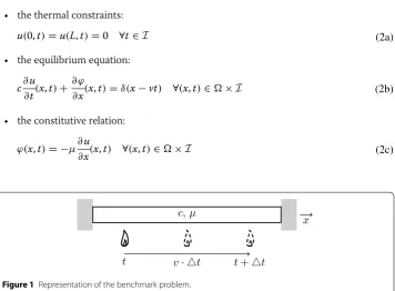
We consider a transient problem defined on a one dimensional domain _{= [}0,L], with boundary ∂�_{= {}0;L}, over the time interval I _{= [0,T]}. It is assumed that a prescribed zero temperature is applied on ∂� and that the domain is subjected to a time-dependent

thermal loading that consists of a thermal source fd(x,t) in . This loading can be seen as a moving flame/laser beam such that f_d(x,t)₌δ(x₋vt), a Dirac distribution, where v is the velocity of the flame/laser beam (see Figure 1).

For the sake of simplicity, the initial conditions are set to zero. The material that com-poses is assumed to be homogeneous and fully known where c (resp. µ) represents the heat capacity (resp. conductivity) of the material.

The associated mathematical problem consists of finding the temperature-flux pair (u(x,t),ϕ(x,t)), with (x,t)_∈�_×I, that verifies:

• the thermal constraints:

• the equilibrium equation:

• the constitutive relation:

(2a)

u(0,t)=u(L,t)=0 ∀t∈I

(2b) c∂u

∂t(x,t)+ ∂ ϕ

∂x(x,t)=δ(x−vt) ∀(x,t)∈�×I

(2c)

ϕ(x,t)_{= −}µ∂u

∂x(x,t) ∀(x,t)∈�×I

c,µ

t v_· t t+t

x

• the initial condition:

In the following, in order to be consistent with other linear problems encountered in Mechanics (linear elasticity for instance), we reform the variable ϕ→ −ϕ which leads, in particular, to the new constitutive relation ϕ₌µ∂_∂xu.

Defining V_=H1

0(�)= {w∈H1(�),w|∂�=0}, the weak formulation in space of the previous problem reads for all t∈I:

with u|t=0=0. Bilinear form b(·,·) and linear form l(·) are defined as:

As regards the full weak formulation, functional spaces T _=L2₍I₎ and L2(I_;V)₌V_⊗T are introduced. The solution _u∈L2(I_;V) is therefore searched, with ∂u

∂t ∈L

2_(I;L2_{(�)), such that:}

with

The exact solution of (4), which is usually out of reach, is denoted uex (and ϕ_ex=µ∂uex

∂x ). It may be approximated using the finite element method (FEM), considering time and space discretizations. Using the classical Galerkin approximation, approximate spaces are introduced: V_h⊂V (resp. T_h⊂T ) made from first order polynomials basis of dimension Nx (resp. Nt). The resulting Nx×Nt linear system leads to a costly brute-force evaluation when Nx and/or Nt are large. Such a solution can be represented as a

Nx×Nt matrix of the following discrete values:

Optimal reduced solution

Let us suppose that the full discrete approximated solution uh is known (under the form

U), and one looks to extract basis functions such as _uh can be approximated under the

separated representation form (1).

The problem consists of defining the separated representation um (1) of the solution

uh of (3) as the one which minimizes the distance to the approximated solution uh with respect to a given norm � · � on V_⊗T.

(2d) u(x, 0)=0 ∀x∈�

(3) Findu(x,t)∈V_{such thatb(u,w)=l(w) ∀w∈}V

b(u,w)=

�

c∂u ∂tw+µ

∂u ∂x

∂w ∂x

dx, l(w)=

�

δ(x−vt)wdx

(4) B(u,w)=L(w) ∀w∈L2(I_;V)

B(u,w)=

I

b(u,w)dt+

�

u(x, 0+)w(x, 0+)dx, L(w)=

I

l(w)dt

U₌



  

uh(x1,t1) uh(x1,t2) · · · uh(x1,tNt) uh(x2,t1) uh(x2,t2) · · · uh(x2,tNt)

..

. . .. ...

uh(xNx,t1) · · · uh(xNx,tNt) 

where functions ψi and i are the optimal reduced basis functions with respect to the chosen norm.

The SVD is a method that transforms correlated data into uncorrelated ones, identifies and orders the dimensions along which data points exhibit the highest variations. From a mathematical point of view, this method is just a transformation which diagonalizes a given matrix A of size _M×N and brings it to a canonical form [24]:

wherea W (resp. V) is a unitary matrix of size _M×M (resp. _N×N) consisting of the r first right (resp. left) singular vectors, r being the rank of A, and is a diagonal matrix

formed by the singular values σi of A such that _{σ1≥σ2≥ · · · ≥σr≥0}.

Since singular values are arranged in a specific order, a best approximation Ak of the

original data points A using fewer dimensions can be determined by simply ignoring

singular values below a particular threshold (k≤r) to massively reduce the data while preserving the main behavior of A. The implied matrix Ak of rank k verifies the Eckart–

Young theorem according to the Euclidean norm � · �2 [25]:

Therefore, if the singular values decreases rapidly, a good approximation of A with small

rank can be found.

For physical problems, the energy norm � · �E is the natural norm in which

measur-ing the error between uex and uh. Therefore, to compare SVD and PGD algorithms, we choose the associated energy scalar product, denoted ��·,·��E, that verifies the variable

separation property:

The implied discrete inner products �·,·�V_h and �·,·�T_h can be written:

where K_∈RNx2 (resp. M_∈RNt2) is the finite element stiffness matrix (resp. the finite ele-ment mass matrix in time) and u_,w_∈RNx×Nt the FEM solution. Employing a Cholesky

(5) �u_h(x,t)₋um(x,t)�2=min

ψi,i

u_h(x,t)₋

m

i=1

ψi(x)i(t) 2

A₌WV†

(6) min

rank(X)≤k�

A_{−X�2= �}A₋A_k�2=σ_k+1

(7a) ��u,w��E =�u(t),w(t)�V,�u(t),w(t)�V

T

(7b) �u(x,t),w(x,t)�T =

I

u(x,t)w(x,t)dt

(7c) �u(x,t),w(x,t)�V=

�

∂u ∂x(x,t)

1 µ

∂w ∂x(x,t)dx

factorization, the inner product ��·,·��E can be transformed to the standard Euclidean

inner product as:

To avoid the use of the Euclidean norm in (6) and thanks to the transformation (8), ones can compute the reduced SVD according to the energy norm through the regular SVD algorithm on the matrix √KU√M rather than on the matrix U. Therefore, the

sepa-rated variable decomposition obtained from the regular SVD verifies:

Matrices and that contain the reduced basis functions ψi and i introduced in (1), have to verify the following relations:

Remark 1 The reduced basis functions ψi∈Vh (resp. i∈Th) are orthogonal with respect to the inner product �·,·�V_h (resp. �·,·�T_h).

Classical PGD methods

Usually, the brute force solution uh is out of reach. In this section, classical PGD strate-gies are reviewed, aiming to approximate the solution u under the form um that verifies

(1) without knowledge of the solution u. In these methods, the reduced basis is com-puted on the fly as the problem is solved.

Rather than solving the m basis functions at once, which is not practical for large scale applications because of prohibitive computational cost, PGD algorithms are built on a progressive algorithm [20]. Assuming that a decomposition um is known (previously

computed), a new couple (ψ,_)∈V_×T is searched such that u is of the form (PGD decomposition of order m+1):

In the following and for clarity reasons, the functions dependency is no longer indicated.

Galerkin PGD

First, a PGD computational method based on Galerkin orthogonality [11] and well-suited for diffusion-dominated problems is presented. By injecting the separated vari-able form (9) in (4), the new couple (ψ,)_∈V_×T is the optimal one that verifies the Galerkin orthogonality:

That equation naturally leads to the following problems :

• the weak formulation of a partial differential equation (PDE) in space, usually

approx-imated by FEM:

(8) �u_�V_h= �

√

Ku_�2, _�u_�T_h= �u √

M_�2

(9) u(x,t)_≃um+1(x,t)=um(x,t)+ψ (x)(t)

• the weak formulation of ordinary differential equation (ODE) in time:

A couple (ψ,_)∈V_×T then verifies (10) if and only if _ψ verifies (11) and verifies (12), which is a non-linear problem. As this problem can be interpreted as a pseudo-eigenproblem [22], a natural algorithm to capture the dominant eigenfunction consists of a power iterations strategy. Starting from an initial random time function (verify-ing initial conditions), each iteration of the power algorithm verifies a sequence of lower dimensional problems (11–12), leading to Algorithm 1.

Remark 2 The key property of Galerkin computational method is that the error is orthogonal to the approximation spaces. Therefore, uex−um is orthogonal to Vh⊗Th according to B(·,·) scalar product.

(11) Bum+ψ,ψ∗=Lψ∗ ∀ψ∗∈V

(12) Bum+ψ_,ψ∗_=Lψ∗ _∀∗_∈T_.

Remark 3 Normalization of space ψ or time functions is preferable for stability rea-son of the power iterations algorithm. In Algorithm 1, we arbitrarily choose to normalize the space function ψ.

Remark 4 One could check the convergence of ψ to stop the power iterations. As explained in [22], a coarse criterion is sufficient to obtain good approximation as conver-gence is reached quickly. In practice, we rather prefer to fix a number of sub-iterations

kmax=4, letting the next PGD mode to correct the previous one if necessary.

Improvement of the decomposition

A post-processing of the computed functions can be made to improve the decomposition, like orthogonalization of space basis functions. A simple modification to the power itera-tions algorithm consists in updating the whole set of time funcitera-tions �m= {i}i₌1...m after

every n-th new PGD mode. These functions are defined by a system of ODEs of dimen-sion m analogous to (12). A mapping application T is defined taking the whole set of space functions �m= {ψ}i=1...m∈Vm into time functions �m=T(�m)∈Tm defined by:

This post-processing improves the quality of the progressive PGD algorithm, although the obtained decomposition is not the optimal one. If the update step is done after each new PGD mode, it is added after the power iterations step, as shown in Algorithm 2. Known as update step [26], it can be applied to all PGD computational methods.

Minimal residual PGD

The next technique is a PGD strategy based on a minimal residual criterion [21]. This construction presents monotonic convergence of the decomposition in the sense of residual norm.

The residual R(u)_∈V_⊗T is defined under the form:

Therefore, an optimal couple (ψ,_)∈V_×T is defined as the one that minimizes the residual norm:

or equivalently:

In a continuous framework, (14) leads to a non-classical formulation as it requires the introduction of a more refined functional space of the space domain V in order to

guar-anty existence and uniqueness of solutions (by introducing H2(�)_⊗H1(I₎ in place of H1(�)_⊗L2(I) for our benchmark problem). In practice, a minimal residual formulation

is applied to the discretized problem (4) after introducing approximation spaces Vh and Th. Therefore, by introducing the discrete NxNt×NxNt matrix B (resp. NxNt vector L) of the bilinear operator B(·,·) (resp. the linear operator L(·)), the discrete NxNt residual vector R of R_(·.) takes the form:

��w,R_{(u)�� =L(w)−B(u,w)= ��w,δ−}

k∂u

∂x +c

∂u

∂t

B_(u)

��

(ψ,_{)=arg min} ψ, �

R_(um+ψ)�2

(14)

(ψ,)₌arg min ψ,

1

2��B(ψ), B(ψ)�� − ��R(um), B(ψ)��

R_(u)=Bu₋L_, u₌ 

 

u_(t1) u_(t2)

.. .



such that an optimal couple (ψ,_)∈V_h×Th minimizes the discretized residual norm (Euclidean norm, since the matrix B is not invertible):

By introducing notation u_m+1=u_m+ψ_·, the minimization leads to the problem:

Let us define the Nx×Nx matrices Cij and the Nx vectors Fi such that:

The discrete minimization (15) leads to the following reduced problems:

• a discretized space problem:

• a discretized time problem:

Remark 5 As for all Galerkin based methods, the error uex−um is orthogonal to the approximation space BTB(V_h⊗T_h) according to the Euclidean scalar product, and depends strongly on the conditioning of the operator BTB_.

(ψ,)₌arg min

ψ, �

R_(um+ψ)_�2₂

(15)

ψ∗_·+ψ_·∗TBTB(u_m+ψ_·)₋BTL₌₀

BTB₌



  

C₁₁ C_{12 · · ·}

C₂₁ . .. ..

. . ..



  ,

BTL₌ 

 

F₁ F₂ .. .



 

(16)



�

i,j

_ijC_ij



ψ=� i

_iF_i

(17) 

  

ψTC₁₁ψ ψTC₁₂ψ _{· · ·}

ψTC₂₁ψ . .. ..

. . ..



  

₌



 

ψTF₁

ψTF₂

.. .



Petrov–Galerkin PGD

In this section, another possible PGD computational method is presented, based on a Petrov–Galerkin criterion, also called MinMax [22]. Such a formulation is frequently used for solving PDEs which contain terms with odd order, implying a loss of symmetry in the weak formulation, as transport-dominated problems.

This Petrov–Galerkin formulation uses the weak formulation (4) where the unknown u and test function w are in different finite dimensional subspaces. Under the variable separation assumption, the test function w is taken as another couple of space and time functions (ψ˜,˜)_∈V_×T such that the new PGD couple _(ψ,)_∈V_×T is the optimal one that verifies the Galerkin orthogonality:

This leads to the two following orthogonality criteria:

As a matter of fact, additional equations must be added in order to define the new functions (ψ˜,˜)_∈V_×T. The following orthogonality criteria (20a), (20b) are used, where ��·,·�� is an inner product on V_⊗T. To compare PGD computational methods one another, we select the energy inner product (7a)–(7c).

As for previous algorithms, an approximation of (ψ,ψ˜,_,˜)_∈V2_×T2 _{is computed} to verify (18) and (20a), (20b) simultaneously. As such a problem is non-linear, a power iterations strategy is chosen, where the four lower dimension problems are solved itera-tively one after the other (see Algorithm 4).

Remark 6 As for all Galerkin based methods, the error uex−um is orthogonal to an approximation space L_{=ψ˜i⊗ ˜i}

i=1...m of the test space according to the B(·,·) scalar product.

(18) Bum+ψ,ψ˜∗˜+ ˜ψ˜∗

=Lψ˜∗˜_{+ ˜ψ}˜∗ _{∀ ˜ψ}∗_∈V_,˜∗_∈T

(19a) Bum+ψ,ψ˜∗˜

=Lψ˜∗˜ _{∀ ˜ψ}∗_∈V

(19b) Bum+ψ_,ψ˜˜∗_=Lψ˜˜∗ _∀˜∗_∈T

(20a) Bψ∗_,ψ˜˜_=ψ∗_,ψ

E ∀ψ∗∈V

(20b) Bψ∗_,ψ˜˜_=ψ∗_,ψ

Minimisation of the CRE

To control the PGD computational process, specific error indicators have been built in recent years. They particularly assess the error due to truncation of the sum in the sepa-rated decomposition (1). A first robust approach for PGD verification, using the concept of CRE, was proposed in [27, 28] leading to guaranteed and relevant error evaluation. It specificity lies on the way to construct the required dual fields, as ϕ(um)=µ∂_∂u_xm does

not verify equilibrium (3). The solution leads to a variable separation of ϕ(um) with a static formulation, done from and after the classical Galerkin PGD space problem. The obtained data combine with prescribed ones, as displacements, traction and body forces define the starting point to evaluate the reduction error.

In this error estimator, the required dual field is computed after the PGD procedure and then cannot influence the solution. Here we propose to compute and control the PGD procedure on the fly with the CRE estimator.

The equilibrium is reformulated by introducing flux fields τ and Q such that:

We wish to minimize the CRE estimator (22), with the constraint that the flux τ verifies

equilibrium (21), with u a kinematically admissible field written with separated repre-sentation form.

As the flux τ has to verify the equilibrium (21), τ can also be written under the variable

separation form:

(21)

I

�

c∂u ∂tw+

ϕ₋Q

τ

∂w

∂x dxdt=0 ∀w∈V⊗T

(22) (u(x,t),τ (x,t))=arg min

u,τ

I

� 1 µ

τ (x,t)+Q(x,t)−µ∂u ∂x(x,t)

2

Indeed, by injecting assumption (1) into equilibrium (21) with a progressive algorithm solver, τ has to verify, at each PGD stage m, the following equation:

The chosen separated form (23) leads to an interesting condition between Zi and ψi:

Therefore, the progressive algorithm adopted in “Classical Proper Generalized Decomposi-tion methods” also applies on τ. It assumes that decomposition um and τm are known

(previ-ously computed) and it looks for a new couple (ψ,_,Z) such that u verifies (9) and τ verifies:

A full minimization

Minimizing the CRE (22) under conditions (25) leads to minimizing the following equa-tion for ψ _∈V, _∈T and Z where the constraint is taken into account through Lagrange multipliers:

Solving the saddle point problem (27) according to each unknown leads to:

• According to :

• According to ψ:

(23) τ (x,t)_≃τ_m(x,t)₌

m

i=1 d_i

dt(t)Zi(x)

(24)

∀k,∀t,

� k

i=1

cdi

dt ψi

w+τ∂w

∂x dx=0, ∀w∈V

(25) ∀i,∀t,

� Zi(x)

∂w

∂x +cψi(x)wdx=0, ∀w∈V

(26) τ (x,t)_≃τm+1(x,t)=τm(x,t)+

d dt(t)Z(x)

(27) (ψ,_,Z,w)₌arg min

ψ,_,Zmaxw

I � 1 µ

Q₊τm−µ

∂um

∂x +

d

dtZ−µ dψ dx 2 dxdt + � Zdw

dx +cψwdx

(28a) 0₌ I � 1 µ

Q₊τm−µ

∂um

∂x + d

dtZ−µ d_ψ

dx _d∗

dt Z−µ

∗dψ

dx

dxdt

∀∗_∈T

(28b)

0₌2

I

�

µ∂um

∂x −Q−τm−

d

dtZ+µ

dψ

dx

dψ ∗

dx dxdt

+

�

cψ∗wdx

• According to Z:

where S ₌

w∈L2(�)| ∀g∈L2(�),

�

gd_dw_x dx=0

.

• According to w:

As (28b)–(28d) are linked together, discrete finite element solutions (ψh,Zh,wh) are determined at once by inverting a matrix problem of thrice the problem size in space:

It should be noted that contrary to the usual case of CRE, discretization errors are not taken into account there. As a matter of fact, very refined space and time meshes will be taken to omit it.

A partial minimization

The full minimization leads to invert a huge problem. In the general case, it is computa-tionally expensive. We propose here a partial minimization where condition (21) is not taken into account in the minimization process but afterwards. That leads to a new and promising PGD computational strategy.

Minimizing (22) under constraint (25) leads to the minimization in V_⊗T _⊗S of:

Minimization (29) leads to:

• According to :

• According to ψ. The field Z is fixed to the previous value computed at the previous

iteration of the power iterations algorithm in first place:

(28c)

0₌2

I � 1 µ

Q₊τm−µ

∂um

∂x + d

dtZ−µ d_ψ

dx

_d

dtZ

∗_dxdt

+

�

Z∗∂w

∂x dx ∀Z

∗_∈S

(28d) 0=

� Z∂w

∗

∂x +cψw

∗_{dx ∀w}∗_∈V_.

B   ψ_h Z_h w_h 

=L

(29) (ψ,_{,Z)=arg min}

ψ,_,Z I � 1 µ

Q+τ_m−µ∂um

∂x +

d

dtZ−µ

dψ dx 2 dxdt (30) 0₌ I � µ

Q₊τm+∂

∂tZ−

∂um ∂x −

dψ

dx

Zd ∗

dt −µ

dψ

dx ∗

dxdt

• One can then determine Z to verify (25).

(31)

0₌

I

�

∂um

∂x +

dψ

dx−Q+τm+

∂

∂tZ

dψ

∗

dx dxdt ∀ψ

∗_∈V

•

Remark 7 The CRE quantity ϕm−µ∂∂umx =τm+Q−µ

∂um

∂x is orthogonal to V⊗T

and S_⊗T approximation spaces according to the energy scalar product.

Remark 8 For stationary problems, condition (24) does not apply. The idea is to seek

τ _∈S0 of the form:

where each Z˜i∈S0=

w_∈L2_(�,I_{)| ∀z∈L}2_(�,I_), I

�

w∂_∂xzdxdt₌0

. Since poten-tial and complementary energies are decoupled, each Z˜i is decoupled from ψi.

A non‑separable lifting algorithm

In this section, a solution of the benchmark problem is computed under the sum of two contributions:

• an enrichment function, determined analytically in an infinite domain, which does

not verify the separated decomposition;

• an additional function, that aims at verifying the boundary conditions, and which

verifies variables separation.

• For the specific benchmark problem defined in (2a)–(2d), we look for the solution in

an infinite domain without space boundary conditions. Let us set X=x−vt such

that U(X)=U(x−vt)=u(x,t). The problem then reads:

τ _≃τ_m= m

i=1 ˜ Zi(x,t)

cvd_dU_X +µd2U

dX2 = −δ(X)

The solution of such an ODE is straightforward, leading to the following equation, where θ stands for the Heaviside function and K is a real constant.

Therefore, a dedicated algorithm is proposed, called Lifting PGD, where the solution is computed with one of the previous PGD algorithms initialized by u_∞ with K =0, i.e. removing the homogeneous solution. To respect boundary conditions in space, u_∞ is

mul-tiplied with ad-hoc functions. As the solution u is equal to u_∞ far from the boundary

con-ditions, u is searched under a specific form to correct u_∞ near the boundary conditions.

To compute the space and time basis functions ψi and i, one can select one of the previ-ously presented PGD strategies.

Results and discussion

On the benchmark problem presented in “The benchmark problem”, we compare the behavior of the different PGD strategies detailed in this paper. The comparison focuses on: (i) quality of approximation by studying the convergence of the Greedy algorithm; (ii) computational cost. Finally, the influence of time effects is studied through the load-ing velocity parameter, to show the main limitations of PGD.

The reference solution u is the classical Galerkin approximation uh, solution of (3), obtained through a brute force FEM. To avoid influence of discretization error, very refined space and time meshes are chosen.

After defining some error indicators, performances of the different PGD strategies are conducted on the benchmark problem with L=3.14m, T =1s, c=0.1Jm−3K−1, µ₌1Wm−1K−1, v= _2TL to form a reasonable test case. Later in “Limits of the Proper Generalized Decomposition”, the influence of these coefficient values will be studied to illustrate limits of the PGD method.

Error estimation

To evaluate the quality of approximation, some error indicators are defined:

Reference reduction error

Since the reference solution is known, an exact reduction error can be defined as the distance between the reference uh and the reduced solution um according to the energy norm. As the mesh is highly refined, this reduction error is the exact one:

Residual error

estimator In general, the reference solution the equilibrium defects of the approximate solution uh is not at hand. Using um, an approximated measure of the real error can be performed without knowledge of the reference solution.

u_∞(x,t,K)₌ θ (x)+K

cv

1−exp−cvµx

− θ (x−vt)+K

cv

1−exp−cvµ(x−vt)

u(x,t)≈u_∞(x,t, 0)×δ(x)×δ(L−x)+um(x,t)

eref = �uh−um�E, eref = eref �uh�E

eres= �R(um)�L2, e_res=

Constitutive Relation As explained in “Minimisation of the Constitutive Relation Error estimator Error”, minimizing the CRE leads to an immediate error

esti-mator, evaluated without knowledge of the reference solution, as:

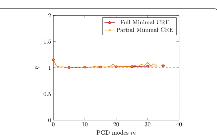
As the exact reduction error is available, one can also define an effectivity index η in

order to quantify the quality of the error estimators. Due to the use of a L2 norm to evaluate the residual error estimation, we only define the effectivity for the CRE estima-tor as:

An error estimator is (i) even more relevant and accurate as the value of its associated effectivity index η is close to 1; (ii) said guaranteed when the value of η is above 1.

Influence of the update phase

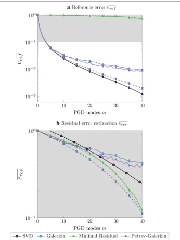
First we propose to compare the classical PGD computational methods presented in “Classical Proper Generalized Decomposition methods”, with or without the update step (see “Improvement of the decomposition”). Convergence curves are given in Figure 2 for a specific value of velocity set to v=L/2T for both reference and residual error estima-tors for classical PGD computational methods.

In Figure 2a, the first 10 modes of Galerkin/Petrov–Galerkin computational methods are close to the optimal decomposition obtained by SVD. Although extra modes degrade that convergence, they tend to follow the same path. Very poor convergence is observed for the classical Minimal Residual PGD computational method according to the refer-ence error e_ref. For Galerkin/Petrov–Galerkin PGD computational methods, the update

step improves significantly the quality of the PGD approximation without fitting the optimal one from SVD. They seem to result in the same PGD decomposition as the error is identical. To get an error of 1%, those two methods need 20 modes when the SVD requires 18 modes.

In general, the reference solution is unknown and convergence plots in Figure 2a can-not be obtained. Reduction error is therefore estimated through the residual error esti-mator eres as represented in Figure 2b. An estimation about 40 times larger than the

reference one for all computational methods is observed. The residual error eres predicts

that the best PGD decomposition comes from the Minimal Residual PGD computational method as it minimizes the residual, even if the reference reduction error says other-wise. The update step for this specific method does not improve the PGD decomposi-tion. On the contrary, the update step highly improves Galerkin/Petrov Galerkin PGD computational methods to the same convergence curve, with a PGD decomposition bet-ter than the Minimal Residual PGD one. According to the residual error estimator, the SVD decomposition is not the optimal one, since we build it according to the energy norm rather than Euclidean norm.

eCRE= �τm−µ ∂um

∂x �E, eCRE=

eCRE �τm+µ∂∂umx �E

η₌ eCRE

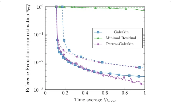
As the purpose of reduction model is to reduce the computational cost of a brute force approximated solution, Figure 3 shows the computational cost of each PGD computa-tional method where the time is averaged by tSVD, the time required to compute a brute

force solution and the separated form through SVD.

In Figure 3 the reference reduction error is plotted as a function of the averaged time to reach it. For the same error level, the consideration of the update step for Galerkin/ Petrov–Galerkin PGD computational method requires more computational time than

0 10 20 30 40

10−3

10−2

10−1

100

PGD modesm

e

f

a Reference error

0 10 20 30 40

10−1

100

PGD modesm

e

s

b Residual error estimation

SVD Galerkin Minimal Residual Petrov-Galerkin

the classical method. However, when using the update step fewer PGD modes are required than without update, thus enhancing storage footprint of the solution and post-processing manipulation.

The update step improves drastically the PGD solution and, in the author opinion, should always be used. In the following, the PGD computational methods will only refer to the PGD one with time function update step, unless otherwise specified.

Minimal CRE performances

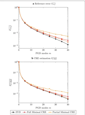
In “Minimisation of the Constitutive Relation Error” we proposed a new PGD com-putational method based on the minimization of CRE, with two variants. In Figure 4, the convergence of each Minimal CRE PGD variant is represented with or without the update step.

We observe in Figure 4a, that the first 10 modes of Full/Partial Minimal CRE PGD computational methods are close to the optimal decomposition obtained by SVD. How-ever extra modes degrade that convergence as the full minimization is better than the partial one. One should observe that when the update step is used, full and partial mini-mizations have the same convergence rate. As a matter of fact, the partial minimization with update gives similar results as the full minimization with update, for a lower com-plexity (Figure 5). Despite the absence of computational time gain in 1D, we hope that the partial minimization will present a better computational time in higher dimension.

In general, the reference solution is unknown and convergence plots in Figure 4a can-not be obtained. Since the new proposed Minimal CRE PGD computational methods have their own reduction error estimation (see “Minimisation of the Constitutive Rela-tion Error”) evaluated through the CRE indicator, the reducRela-tion error is therefore esti-mated through the CRE estimator eCRE as represented in Figure 4b. As seen in Figure 4a,

the update step improves the convergence of the computational methods close to the

0 0.2 0.4 0.6 0.8 1

10−3 10−2 10−1 100

Time averaget_{/tSV D}

Reference

Reduction

error

estimation

ere

f

Galerkin Minimal Residual

Petrov-Galerkin

reference one. As a matter of fact, they are effective (accurate and guaranteed) as shown in Figure 6.

As a result, in the general case, one can only evaluate some error estimators depend-ing on the computational methods. Then the CRE indicator obtained by minimizdepend-ing the CRE leads to an improved and accurate reduction error estimation. Other PGD com-putational methods errors underestimate the reduction error. Unlike the Minimal CRE PGD solution, they require to compute extra modes to target a specific reference error.

0 10 20 30 40

10−3

10−2

10−1

100

PGD modesm

e

f

a

0 10 20 30 40

10−3

10−2

10−1

100

PGD modesm

e

E

b

SVD Full Minimal CRE Partial Minimal CRE

Figure 4 Convergences of Minimal CRE PGD computational methods for the exact error e_ref (a) and the CRE

estimator eCRE (b). Dashed lines represent the update of time functions version, solid lines represent the PGD

The two CRE minimization strategies show great performances, robustness from min-imization and give direct effective error estimator.

Limits of the PGD

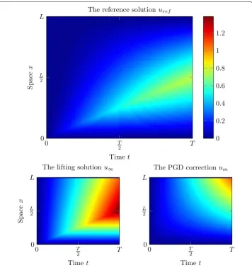
In “A non-separable lifting algorithm”, we proposed a PGD computational method lifted with a non-separable known solution. Figure 7 represents the enrichment solution u_∞

solution over an infinite domain and the correction PGD solution um computed with a

Galerkin PGD strategy with time functions update step. 3 modes are enough as the PGD

0 0.2 0.4 0.6 0.8 1

10−3 10−2 10−1 100

Time averaget_{/tSV D}

Reduction

error

estimation

eCR

E

Full Minimal CRE Partial Minimal CRE

Figure 5 Normalized computational cost of PGD methods according to the reduction error from CRE estimator eCRE. Dashed lines represent the update of time functions version, solid lines represent the PGD com‑

putational method without update.

0 10 20 30 40

0 0.5

1 1.5

2

PGD modes m

η

Full Minimal CRE Partial Minimal CRE

solution matches the reference solution uref below a relative reference error of 10−3. It

is easy to observe that the correction term verifies the separation of variables from Fig-ure 7, as the solution is smooth and continuous.

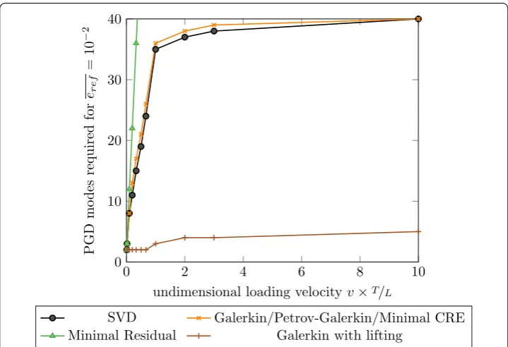
In Figure 8, the number of PGD modes required to obtain a reference error eref below

10−2 is studied depending on the loading velocity. While SVD and PGD computational methods require much more modes to catch the influence of the speed when the veloc-ity increases, the lifting method only requires 2 PGD modes to get an accurate solution below a relative reference error of 10−2. Such properties come from the lifting solution

u_∞ that catches the influence of the speed. According to (6), the 35th singular value of u_∞ is below 10−2 _{for v=} L

2T. It should be noted that when the velocity of the loading is greater than one, the flame leaves the domain. As a results, a plateau appears after that value.

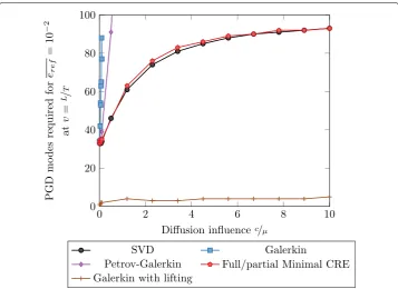
Therefore, we rather propose to study the influence of the instationary term in the equilibrium equation (2b). To do so, we study the number of PGD modes required to meet a target error of 10−2 _{according to the diffusion coefficient c/µ, as shown in}

0 T

2 T

0 L 2

L

Timet

Space

x

The reference solutionuref

0 0.2

0.4

0.6

0.8

1 1.2

0 T

2 T

0 L 2

L

Timet

Space

x

The lifting solutionu∞

0 T

2 T

0 L 2

L

Timet

The PGD correctionum

Figure 9. While classical PGD methods have difficulties to catch the right solution, minimizing the CRE leads to a better solution close to the optimal SVD one. As previ-ously noted, the lifting technique requires much less modes to catch the solution, and does not depend of the influence of the diffusion term. Even if SVD or PGD computa-tional methods require less modes to reach such an error, the lifting technique has the advantage not to compute those modes and therefore does not depend on the loading velocity.

From Figures 8 and 9, we study the influence of the transient part of the solution. Such a part does not verify the assumption of separated variables representation. When the diffusion term is neglectable, time does not influence the solution and a separated rep-resentation is implicit. On the other hand, time cannot be longer neglected, and extra separated modes are required.

In this section, the assumption of variable separation shows its limits for instation-ary problems that do not verify such an assumption. Initializing PGD strategies with a known unseparable solution circumvents that limit. Such more thoughtful strategy, pre-sented as a lifting PGD technique, shows that the PGD method is not faulted.

Conclusion

We reviewed different possible PGD computational methods for the a priori con-struction of reduced order time-dependent thermal model (ROM) based on the separated representation of the related solution. Different constructions have been analyzed, based on Galerkin, Minimal Residual and Petrov–Galerkin formulations

0 2 4 6 8 10

0 10 20 30 40

undimensional loading velocity v×T_/L

PG

Dm

odes

required

for

ere

f

=1

0

−

2

SVD Galerkin/Petrov-Galerkin/Minimal CRE

Minimal Residual Galerkin with lifting

Figure 8 Number of PGD modes required to target a reference error eref below 10− 2

of the evolution problem. They were compared on a one dimensional benchmark problem.

The numerical example has illustrated the importance of selecting a relevant and accu-rate reduction error estimator, as it is required to know when to stop the progressive algorithm. As the reference error estimator is generally out of reach, classical PGD com-putational methods usually lie on residual error estimator. As a matter of fact, this esti-mator is not effective nor accurate.

We proposed an innovative PGD construction based on minimizing the CRE. Its main advantage is to provide a robust, accurate and relevant reduction error indicator while maintaining advantages of PGD. Due to the use of CRE, discretization error is within easy reach and allows adaptive construction of PGD decomposition.

The update step highly improves convergence properties of all PGD computational methods. Putting aside the Minimal Residual PGD, all PGD computational methods coupled with this update step converged to the same PGD decomposition. It has the same convergence properties as an optimal reduced solution obtained by SVD.

Finally, limitations of PGD computational methods have been illustrated by lift-ing Galerkin PGD computational method with a non-separable solution. Convergence of PGD computational methods tends to decrease when the separation of variables assumption cannot respect the problem to solve. We illustrated it for a time dependent problem, but parameters dependent problems may have the same behavior.

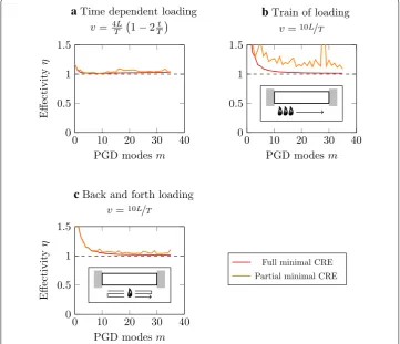
Further analysis of the Minimal CRE PGD computational method was conducted for different loading types and confirms its performances as shown in Figure 10. Future

0 2 4 6 8 10

0 20 40 60 80 100

Diffusion influencec_/µ

PG

Dm

odes

required

for

ere

f

=1

0

−

2

at

v

=

L/

T

SVD Galerkin

Petrov-Galerkin Full/partial Minimal CRE

Galerkin with lifting

work will be devoted to the extension of the newly proposed PGD computational method (CRE) to non-linear and multi-parameter problems.

Endnote

a_Here, V† denotes the adjoint matrix of V.

Authors’ contributions

All authors have read and approved the final manuscript.

Compliance with ethical guidelines Competing interests

The authors declare that they have no competing interests.

Received: 30 January 2015 Accepted: 29 June 2015

References

1. Krysl P, Lall S, Marsden J (2001) Dimensional model reduction in non‑linear finite element dynamics of solids and structures. Int J Numer Methods Eng 51(4):479–504

2. Ryckelynck D (2005) A priori hyperreduction method: an adaptive approach. J Comput Phys 202(1):346–366 3. Boyaval S, Bris CL, Maday Y, Nguyen NC, Patera AT (2009) A reduced basis approach for variational problems with

stochastic parameters: application to heat conduction with variable robin coefficient. Comput Methods Appl Mech Eng 198(41):3187–3206

0 10 20 30 40

0 0.5 1 1.5

PGD modesm

Effectivit

y

η

a

b

c

T

0 10 20 30 40

0 0.5 1 1.5

PGD modes m

v=10L_/T

0 10 20 30 40

0 0.5 1 1.5

PGD modesm

Effectivi

ty

η

v=10L_/T

Full minimal CRE Partial minimal CRE

4. Kunisch K, Volkwein S (2001) Galerkin proper orthogonal decomposition methods for parabolic problems. Numer Math 90(1):117–148

5. Sanghi S, Hasan N (2011) Proper orthogonal decomposition and its applications. Asia Pac J Chem Eng 6(1):120–128 6. Maday Y, Rønquist E (2002) A reduced‑basis element method. J Sci Comput 17(1–4):447–459. doi:10.102

3/A:1015197908587

7. Rozza G, Huynh DBP, Patera AT (2008) Reduced basis approximation and a posteriori error estimation for affinely parametrized elliptic coercive partial differential equations. Arch Comput Methods Eng 15(3):229–275. doi:10.1007/ s11831‑008‑9019‑9

8. Chinesta F, Ladeveze P, Cueto E (2011) A short review on model order reduction based on proper generalized decomposition. Arch Comput Methods Eng 18(4):395–404. doi:10.1007/s11831‑011‑9064‑7

9. Chinesta F, Ladevèze P (eds) (2014) Separated representations and PGD‑based model reduction, vol CISM554. Springer, Udine

10. Ladevèze P (1989) The large time increment method for the analysis of structures with non‑linear behavior described by internal variables. Comptes Rendus de l’Académie des Sciences Série II 309(11):1095–1099

11. Ladevèze P (1999) Nonlinear computational structural mechanics: new approaches and non‑incremental methods of calculation. Springer, Berlin

12. Néron D, Ladevèze P (2010) Proper generalized decomposition for multiscale and multiphysics problems. Arch Comput Methods Eng 17(4):351–372

13. Ladevèze P (2014) PGD in linear and nonlinear computational solid mechanics. In: Chinesta F, Ladevèze P (eds) Separated representations and PGD‑based model reduction, vol CISM554. Springer, Udine, pp 91–152

14. Nouy A (2008) Generalized spectral decomposition method for solving stochastic finite element equations: invari‑ ant subspace problem and dedicated algorithms. Comput Methods Appl Mech Eng 197(51):4718–4736

15. Niroomandi S, Alfaro I, Cueto E, Chinesta F (2012) Accounting for large deformations in real‑time simulations of soft tissues based on reduced‑order models. Comput Methods Programs Biomed 105(1):1–12

16. Leygue A, Verron E (2010) A first step towards the use of proper general decomposition method for structural optimization. Arch Comput Methods Eng 17(4):465–472

17. Chinesta F, Ammar A, Cueto E (2010) Recent advances and new challenges in the use of the proper generalized decomposition for solving multidimensional models. Arch Comput Methods Eng 17(4):327–350

18. Vitse M, Néron D, Boucard P‑A (2014) Virtual charts of solutions for parametrized nonlinear equations. Comput Mech 54(6):1529–1539

19. Ladevèze P, Chamoin L (2011) On the verification of model reduction methods based on the proper generalized decomposition. Comput Methods Appl Mech Eng 200(23):2032–2047

20. Temlyakov VN (2008) Greedy approximation. Acta Numer 17:235–409

21. Ammar A, Chinesta F, Falcó A (2010) On the convergence of a greedy rank‑one update algorithm for a class of linear systems. Arch Comput Methods Eng 17(4):473–486

22. Nouy A (2010) A priori model reduction through proper generalized decomposition for solving time‑dependent partial differential equations. Comput Methods Appl Mech Eng 199(23):1603–1626

23. Ladevèze P, Chamoin L (2013) Toward guaranteed PGD‑reduced models. Bytes and Science. CIMNE: Barcelona, pp 143–154

24. Golub GH, Van Loan CF (2012) Matrix computations, vol 3. JHU Press, Baltimore

25. Hubert L, Meulman J, Heiser W (2000) Two purposes for matrix factorization: a historical appraisal. SIAM Rev 42(1):68–82

26. Bussy P, Rougée P, Vauchez P (1990) The large time increment method for numerical simulation of metal forming processes. In: Proceedings of NUMETA, pp 102–109

27. Chamoin L, Ladevèze P (2012) Robust control of PGD‑based numerical simulations. Eur J Comput Mech 21(3–6):195–207