Mesh refitting approach: a simple method to model mixed-mode crack propagation in nonlinear elastic solids

R E S E A R C H A R T I C L E

Open Access

Mesh refitting approach: a simple method

to model mixed-mode crack propagation

in nonlinear elastic solids

Y. Sudhakar

and Wolfgang A. Wall

*_{Correspondence:} [email protected] Institute for Computational Mechanics, Technical University of Munich, Boltzmannstr. 15, 85747 Garching, Germany

Abstract

We devise a finite element methodology to trace quasi-static through-thickness crack paths in nonlinear elastic solids. The main feature of the proposed method is that it can be directly implemented into existing large scale finite element solvers with minimal effort. The mesh topology modifications that are essential in propagating a crack through the finite element mesh are accomplished by utilizing a combination of a mesh refitting procedure and a nodal releasing approach. The mesh refitting procedure consists of two steps: in the first step, the nodes are moved by solving the elastostatic equations without touching the connectivity between the elements; in the next step, if necessary, quadrilateral elements attached to crack tip nodes are split into triangular elements. This splitting of elements allows the straightforward modification of element connectivity locally, and is a key step to preserve the quality of the mesh throughout the simulation. All the geometry related operations required for crack propagation are addressed in detail with full emphasis on computer implementation. Solving several examples involving single and multiple cracks, and comparing them with experimental or other numerical approaches indicate that the proposed method captures crack paths accurately.

Keywords: Mesh refitting method, Crack propagation in nonlinear materials, J-integral, Nodal releasing technique, Fracture of nonlinear solids

Background

Objective and motivation

One of the main reasons why devising a computational methodology to deal with fracture mechanics is challenging, is the fact that cracks propagate in arbitrary directions through the material. If the dynamics of the crack were known apriori, one can design an optimal mesh that allows the propagation of a crack through the pre-existing mesh at each instant. Since this is not the usual case, the mesh has to be repeatedly modified to accommodate the advancement of cracks within the finite element (FE) mesh. The objective of this work is to devise a simple procedure to achieve the required mesh modifications, which enables us to model complex crack paths through nonlinear elastic solids. The present work is motivated by our interest in developing computational methodologies for fluid-structure-fracture interaction (FSFI) [1] that model the following phenomenon: when a flexible structure interacts with the fluid flow, the fluid loading induces elastic deformation

©The Author(s) 2017. This article is distributed under the terms of the Creative Commons Attribution 4.0 International License (http://creativecommons.org/licenses/by/4.0/), which permits unrestricted use, distribution, and reproduction in any medium, provided you give appropriate credit to the original author(s) and the source, provide a link to the Creative Commons license, and indicate if changes were made.

as well as fracture failure of the structure, and the fluid medium fills the crack opening. The first step of extending fluid-structure-interaction (FSI) methods to handle FSFI is to equip the structural analysis with a fracture mechanics solver. This is achieved in this work by developing a crack propagation approach which facilitates, with minimal implementation efforts,

• to update the existing large scale structural mechanics solver into a robust tool to handle single and multiple quasi-static cracks

• to couple the crack propagation method with existing FSI approach to model FSFI.

The method devised in this paper is implemented inBACI, a large scale parallel multi-physics solver developed at our institute. It is to be mentioned that the objective of the present work is not to devise a method which is competitive to the available class of meth-ods in terms of computational efficiency or accuracy. Rather, the focus is on devising a simple crack propagation approach, which circumvents the complexities associated with them (as discussed below) to aid the development of an FSFI solver.

Brief overview of relevant methods

The present work is based on fracture mechanics [2–12] framework rather than on contin-uum damage mechanics [13,14] because we model the propagation of sharp cracks in the material. Majority of the existing computational methods employing fracture mechanics principles utilize either one of the following frameworks:

• Adaptive remeshing • Enriched partition of unity

These methods are very successful and find plethora of applications but implementing them in an existing (large scale) FE package pose several challenges.

Adaptive remeshing methods

These methods, as the name implies, adaptively refine the mesh in the crack tip vicinity where the solution dictates the dynamics of crack propagation, and coarsen the mesh away from the crack tip. They make use of special data structures [2,3,15], together with either a globally adaptive remeshing procedure [4–6] or a local mesh modification algorithm [7] to accommodate crack propagation at arbitrary directions within the computational domain. Each time when a crack extends, these methods introduce several new nodes into the mesh. As a result, they require mesh generation related algorithms to modify the mesh appropriately. Usually in a large scale FE code which is generalized to address multiscale and multiphysics problems, such fracture-specific and mesh-modification routines are neither available nor easy to implement in a generalized way.

Enriched partition of unity methods (EPUM)

can propagate within the interior of an element, and hence it is possible to simulate crack propagation without modifying the underlying discretization. Though these methods are demonstrated to be powerful, the following points hamper their easier implementation into an existing structural mechanics solver. The numerical integration of singular enrich-ment functions is still an active area of research in EPUM [22–28]. Moreover, these meth-ods require the implementation of complicated geometry-mesh intersections for which robustness is always an issue, especially in 3D. Also, the number of degrees of freedom attached to a few nodes changes each time when the crack advances. Most importantly, except a few (e.g. [29–31]), all studies are focused on crack propagation through linear elastic materials mainly because the formulation of enrichment functions in nonlinear regime is still an active area of research.

Owing to the aforementioned implementation issues, neither EPUM nor adaptive remeshing methods are ideal for developing fluid-structure-fracture interaction meth-ods. This is because FSFI methods have to handle the combination of challenges from two sources: those arising from crack propagation besides another big challenge from FSI. The aim of this work is to devise a simple crack propagation approach that is suitable specifically for developing FSFI.

The method developed in this work, as will be explained later, shares a similarity with arbitrary Lagrangian Eulerian (ALE) based methods that it involves a mesh-deformation step. Therefore, ALE based methods for fracture mechanics are briefly recalled. The use of ALE in computational fracture mechanics is not widespread. Only few studies employed ALE to address crack propagation problems, and a brief account of majority of such works is provided below.

Existing ALE based crack propagation methods

of ALE to maintain high nodal density in the preferred region is accomplished effectively without resorting to remeshing strategies (refer to [39] for complications involved in implementing such a method in mesh-based FEM). The method is successfully applied to simulate wave propagation and dynamic crack propagation.

To summarize, to our knowledge neither a complex trajectory of a single crack nor simple propagation of multiple cracks within a material is modeled until now using ALE based methods. This is predominantly due to the fact that the mesh modification method used in ALE, in its classical sense, cannot handle the mesh topology changes that are introduced by advancing a crack through the FE mesh. Continuous remeshing is manda-tory to eliminate the associated mesh tangling problems. In this work, this is avoided by using an additional step in the mesh refitting procedure that allows tomodify the element connectivity locallyto preserve the quality of mesh, as will be explained in the later section.

Structure of the paper

The remainder of the paper is structured as follows. The next section briefs the govern-ing equations and the boundary conditions for the problem. Then the complete crack propagation algorithm together with all the details necessary for computer implementa-tion are presented. Finally several numerical examples to demonstrate the accuracy of the proposed method are described.

Governing equations

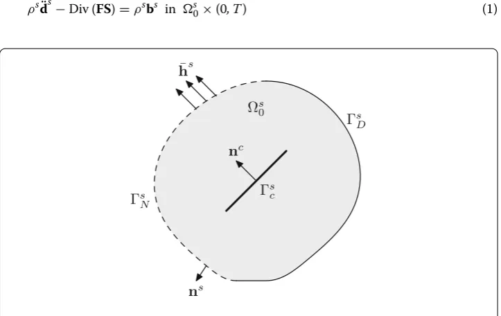
At reference timet = t0, let the structure occupy the domains₀, withsdenoting the boundary of the structure (Fig.1).sis divided into three non-overlapping portions such thats = s_D∪_Ns ∪s_cin which_Ds ands_N are Dirichlet and Neumann portions of the boundary respectively, ands_cdenotes the crack surfaces which contain always two physical crack facess_c=_c+s ∪_c−s . The balance of linear momentum equation is written as,

ρs_d¨s_{−Div (FS)=ρ}s_bs _in s

0×(0, T) (1)

Γ

Γ

Γ

n

n

Ω

¯

h

where ρs_{is the density of the structure,Fis the deformation gradient,Sis the second} Piola-Kirchhoff stress tensor,bs represents externally applied body force per unit mass, ds is the structural displacement andd¨s = d_dt2d2s. T is the end time of the considered

time interval, and Div(·) is the divergence operator defined with respect to the material reference frame.

Since this is an evolutionary problem involving second order time derivative, initial conditions must be specified ondsand its first derivative ˙ds= d_dtds

ds|t=0=ds0 ons0; ˙d s

|t=0=d˙s0 ons0 (2)

Over the boundary of the domain, Dirichlet conditions are specified on_Ds, Neumann conditions are prescribed on_Ns, and the crack surfaces are assumed to be traction-free.

ds=d¯s on_Ds ×(0, T) ; (FS)·ns=h¯s on_Ns ×(0, T) (3a)

(FS)·nc+=0 ons_c+×(0, T) ; (FS)·nc−=0 on_c−s ×(0, T) (3b)

We deal with hyperelastic Neo-Hookean materials in this work. The strain energy function for such material is given as

NH= μs

2 (trC−3)−μ

s_lnJ+λs 2 (lnJ)

2 ₍₄₎

whereCis the Cauchy–Green tensor,Jis the determinant of deformation gradientJ = detF,λsandμsare Lame’s constants.

The mesh refitting approach

The complete numerical methodology, together with the computer implementation aspects, of the present approach are presented in this section. It is assumed that the fracture behavior of the material is completely characterized by theJ-integral.

The focus of the present work is to simulate through-thickness mixed-mode quasi-static crack propagation within a structure. The current work can be considered as an extension of Tabiei and Wu [40] which describes the implementation of a crack module in DYNA3D FE package, and shares similarities with the method of Miehe and Gürses [3]. Both works address crack propagation through linear elastic materials only. Moreover the complex geometry related operations, like deciding the new crack tip nodes, are not addressed in depth. These details are crucial for implementation of the method. The approach proposed in [3] was called anr-adaptive method, but in order to avoid confusion with complexr -adaptive mesh redistribution methods [41,42], the present method is labelled as mesh refitting approach. The following section presents the complete implementation details of the present method. Though we simulate through-thickness cracks, for simplicity we explain the geometry-related operations in 2D.

Algorithm 1Computational crack propagation procedure at each time step 1: Construct local coordinate system at crack tip

2: Compute vectorJ-integral

3: Check whether crack propagates or not, from crack propagation criterion 4: if Crack propagation criterion is not satisfiedthen

5: continue to the next time step 6: end if

7: Obtain the direction of crack propagation from crack kinking criterion 8: Find the new crack tip nodes

9: Apply mesh refitting procedure

10: Propagate the crack using nodal releasing technique

Solve the governing equations

The first step is to solve the structural dynamic equations by freezing the location of the crack. The strong form given in Eq. (1) is multiplied by appropriate test functions (δds) and are integrated over the structural domain to obtain the weak form which is stated as, Findds∈Wdsuch that for allδds∈Vd, the following holds

(δds,ρsd¨s)s

0+(Gradδd

s_,FS)

s

0 =(δd

s_,ρs_bs₎

s

0+ δd

s_,h¯s s

N (5)

where (., .)s

0 and., .sN mean the standardL

2_{-inner product over the reference domain}

and Neumann part of the boundary, respectively.

The solution space and the test function space are defined as Wd = {ds∈H1(s0)|ds=d¯

s

ons_D} (6)

Vd = {δds∈H1(0s)|δds=0 onDs} (7)

The above integral equations are dealt with nonlinear FEM for spatial discretization and Generalized-α method for time discretization. The resulting nonlinear system of algebraic equations are solved using Newton–Raphson method to obtain the solution of displacement field (ds). For a more elaborate discussion of this well established procedure, the reader can refer to the literature (e.g. [43,44]).

Perform computational crack propagation procedure

The displacement solution obtained from the previous step is used to perform crack propagation procedure by computing vectorJ-integral. It involves seven discrete steps, each of which are detailed below.

Step 1: Construct local coordinate system at crack tip

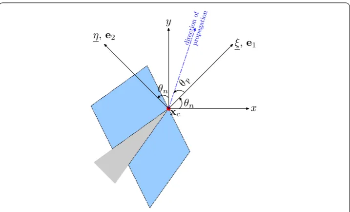
To compute fracture mechanics quantities from the FE solution, and to decompose these quantities into their corresponding modes in a mixed-mode problem, it is essential to construct a local coordinate system (ξ,η) at the crack tip (xc) as shown in Fig.2. The base vectors (e1,e2) associated with (ξ,η) can be easily constructed becausee1is the symmetry line of the crack; e2 can be obtained by computing the normal toe1 in a right hand coordinate system.

Step 2: Compute vectorJ-integral

propa-xc

x

y

ξ

,

e

η

,

e

θ

θ

θ

direction of

propagation

Fig. 2 Construction of local coordinate system at crack tip. TheshadedQuads represent finite elements

gates or not, and if at all it propagates in which direction it advances. Hence, it is essential to accurately evaluate theJ-integral.

With respect to the spatial configuration, the energy release rate along the direction of a crack is defined as,

J =

γj

wn_ξ−n·σ· ∂d

∂ξ

dγ (8)

whereγjis the integration contour,wis the strain energy stored per unit deformed volume, nis the normal to contourγjandσis the Cauchy stress tensor. All these quantities are defined in the current spatial configuration as shown in Fig.3a. Since the current work

a b

employs a total Lagrangian formulation, it is convenient to express theJ-integral in the reference configuration using pull-back operations. As shown in [30], it reads as

J =

j

WN−N·P· ∂d

∂

d (9)

wherej, W,Nare the corresponding quantities in reference configuration,Pis the first Piola-Kirchhoff stress tensor and (, H) denote the crack tip coordinate system in the reference configuration, which is given by its base vectors (E1,E2) in Fig.3a.

In FEM, the contour integrals are cumbersome to implement because the material variables are available only at the Gauss points. Interpolating these variables over the desired contour presents complications, in addition to introducing interpolation errors. Hence, several studies [46,47] have proposed the idea of converting the contour integral into an integral evaluated over a finite domain around the crack tip by applying the divergence theorem. This procedure is straightforward to implement, as it requires only the quantities at Gauss points of elements within the finite domain. The equivalent domain form ofJ-integral for large deformation problems is given as [29,30],

J =

S

∂d

∂X ·P−WI

·∇0(q)dS (10)

whereSis the domain enclosed byj, and∇0(q) is the gradient of support functionqwith respect to the reference configuration.

In order to constructq, using nodal connectivity information, all the elements that are located onn−layers around the crack tip (see Fig.3b withn= 4) are considered. From this, the elements connected to the crack tip are deleted. Then, all the nodes that are on the outer boundary of this element set are located, and among these nodes, the one which has the shortest distance (rmin) from the crack tip is chosen. Then the support function is initialized to take a value of unity at the inner layer of nodes, and drops smoothly to zero when the distance of a node from crack tip is more than or equal tormin. The distribution ofqwithin the integration domain is given in Fig.3b.

NoteIn this work, we assume that the crack surfaces are traction-free. However, in FSFI applications, fluid loads are acting on the crack faces, and as a result an additional term appear in the computation ofJ-integral. This is explained further in [1].

Step 3: Check crack propagation criterion

The crack propagation criterion determines whether the existing crack propagates through the structure under the current stress state. Crack propagation occurs when the driving force reaches or exceeds the material resistance. The J-integral provides a measure of driving force, and its critical value (Jc) is assumed to be a material property, which quantifies the material’s resistance to crack propagation.

The present work makes use of the vectorJ-integral based crack propagation criterion proposed by Ma and Korsunsky [48]. This criterion requires, first, the calculation of maximum strain energy release rate, which is given by the magnitude of J.

Gmax=

whereJ1andJ2are the strain energy release rates along the direction ofe1ande2 respec-tively, which are given by simple dot productsJ1=J·e1andJ2=J·e2.

The crack extension under the given loading conditions occurs, whenGmaxreaches the fracture toughness of the material (Jc),

Gmax≥Jc (12)

If the crack propagation criterion is not satisfied, then there is no need to perform the remaining operations; the algorithm moves to the next time step to solve the governing equations of the structure.

Step 4: Obtain the direction of crack propagation

After confirming that the crack propagates, the next logical step is to determine along which direction it is going to advance through the material, which is provided by the crack kinking criterion.

There are several methods put forward to determine the crack kinking direction, and the most important methods are

• Maximum circumferential stress criterion [49], • Minimum strain energy density criterion [50],

• Maximum energy release rate criterion (MERR)[48,51].

It is concluded in a comparative study [52] that the minimum strain energy density criterion is less accurate, and the accuracy of maximum circumferential stress criterion and maximum energy release rate criterion are equivalent in all the tests considered.

This work incorporates the maximum energy release rate criterion, proposed in [48], which is consistent with the crack propagation criterion given in the last section. It is stated that the crack propagates whenGmaxreaches or exceeds the characteristic fracture toughness of the material. MERR predicts the crack propagation direction (θp) to be the direction ofJ, which is simply given as

θp=tan−1

J2

J1

(13)

It is to be remembered thatθpis measured with respect to the crack normal, as indicated in Fig.2. Moreover, in this work, the extent of crack propagation is always set to be the length of one complete edge of an element.

Step 5: Find new crack tip nodes

Having computed the crack propagation direction fromJ, the next essential step is to determine the new crack tip nodes i.e, nodes in the FE mesh through which the crack must be propagated. A geometry-based method is used in this work to identify the new tip nodes.

φ

φ

δ

current tip

diagonal nodes

propagation vector

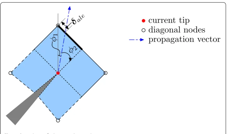
Fig. 4 Procedure to find new crack tip nodes

After getting the required intersecting edge, the next step is to check whether the crack propagates along the diagonal. This is realized by the condition,φ1≤diag-tol(=0.25 radians in all the simulations). In this case, the diagonal node corresponding to φ1 is marked as new tip node. Since the crack propagates through a diagonal of the element, this element must be split along this diagonal to accommodate crack propagation through the mesh, as explained in the next step.

Ifφ1>diag-tol, then the non-diagonal node of the intersecting edge will be the next new tip node. In either cases, all the new tip nodes (if there are multiple cracks, each crack tip will have its own new tip node) are stored inRale. Moreover, the distance between the intersection point and the new tip nodes, marked asδ_alein the figure, are computed and will be used in the next step.

Step 6: Mesh refitting procedure

In this step, we refit the existing mesh in such a way that the modified mesh contains an edge along which the crack can propagate. The mesh refitting procedure used in the present work involves two discrete operations listed as follows:

1. Nodal repositioning

2. Splitting quadrilateral (Quad) elements into triangular (Tri) elements

In the first step, the nodes are repositioned without touching the elements. This means that the element topology (shape and total number of elements, or the connectivity between elements) remains unchanged. The elements only deform due to the movement of the nodes.

∇·σm_{=0 on}s _(14a)

dm=0 on∂ale (14b)

dm=δale onRale (14c)

where σm is the fictitious Cauchy stress tensor,dm denotes the displacements at each node within the mesh,s_{represents the whole structural domain, and∂aledenotes the} boundary for ALE computations:∂ale=s

D∪Ns ∪cs. Displacements at the new crack tip nodes are set to beδalethat is computed in the previous step.

The above equations are solved to obtain the mesh displacementdm, which is used to move each node in the mesh to its new location. After this mesh movement operation, the new crack tip node is moved to the intersection point along the intersection edge (see Fig.4).

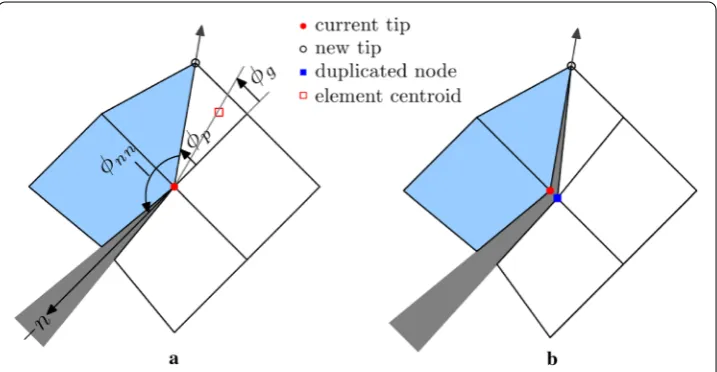
In the next step of the mesh refitting procedure, theQuadelements that are marked to be split are cut into two Tri elements. This happens when the crack propa-gates very close to the diagonal of a Quad element (Fig. 5a). This process does not involve introducing new nodes into the mesh. By comparing Figs.4 and5a, the effect of the mesh refitting procedure is clear: the new tip nodes are first moved to the desired location using the nodal repositioning step, and then the Quad element is appropriately split into Tri elements to enable crack propagation along the diago-nal. In short, the combination of nodal repositioning and element splitting ensure that after the mesh modifications, the crack propagates along an existing edge in the new mesh.

One of the main reasons for the failure of ALE based methods in handling large defor-mation or topology change is that such methods maintain their nodal connectivity during the entire simulation. The element splitting operations used in the present work allevi-ates this problem by enabling us to modify the connectivity between the elements locally. This is an essential step without which the nodal repositioning method cannot handle the change in mesh topology that is inherent to crack propagation problems, without resorting to complicated and time-consuming remeshing procedures.

Step 7: Nodal releasing technique

The two previous steps have enabled us to identify new tip nodes, and to move these nodes to match the computed propagation angle. However, the material separation is not yet included within the FE procedure. In order to achieve this, and to form physical crack surfaces, the nodal releasing technique is used.

In order to represent the material separation, the element connectivity at the current tip node must be modified; a duplicate node is created at the same location where the current tip resides. Few elements are released from the current tip node, and are assigned with a new duplicate node. This, in turn, generates new crack surfaces. In order not to destroy the FE mesh during this process, a consistent way of determining which elements get duplicate nodes is used.

In this procedure, two angles are defined: one isφpalready defined in Fig.4, and the other is the angle formed by the negative normal at crack tip to the propagation vector (φnn in Fig.5a). Then, for each element, the angle (φg) formed by the line connecting current tip to the centroid of the element and the normal is computed. The element is released and gets the duplicate node, ifφg ∈/ [φp,φnn]. The elements that retain the current tip node are shaded in Fig.5a. After nodal releasing and modifying element connectivity, the mesh close to the crack tip is plotted in Fig.5b. At this point, the material separation is introduced and all the crack propagation operation are completed.

Numerical examples

Several examples of varying complexity are solved to demonstrate the effectiveness of the proposed method. These examples exhibit single and mixed-mode behavior, involv-ing mono- and multimaterials. In order to closely examine the accuracy of the method, crack paths obtained from the present method are compared with experiments or results obtained from other methods in literature.

The first two examples consider stationary cracks, and the quantities calculated are compared with XFEM studies [30,31]. These examples consider highly nonlinear effects evident from the crack tip blunting observed in the results. All the other examples involve complex crack propagation through the structure.

Crack tip blunting

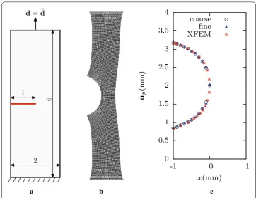
Consider a single edge notched specimen with dimensions 2 mm ×6 mm. The crack occupies half-width as shown in Fig.6a. The top surface is subjected to a fixed displacement of 4 mm. All these details are taken from [30]. The strain energy function of the material is given by,

NH= μs

2 (trC−3) (15)

The Lame parameters are set such thatμs_{=0.4225 MPa and the equivalent Poisson ratio} in the linear regimeν=0.49.

a b c

0

0.5

1

1.5

2

2.5

3

3.5

4

-1

0

1

u

(mm)

x

(mm)

coarse

fine

XFEM

Fig. 6 Crack tip blunting.aGeometry. All dimensions are in mm.bDeformed configuration.cPlot of vertical displacement of crack surface nodes against their horizontal position in reference state. XFEM results for comparison are taken from [30]

from our simulations are matching well with the reported results. Moreover, the simu-lations using coarse and fine mesh yield identical values, which shows that the reported results are converged with mesh density. The coarse and fine mesh contain 1200 and 4800 uniform Cartesian elements respectively. It is to be mentioned that the XFEM study [30] was focused on incompressible materials, and the present results closely resembles the incompressible condition by takingν=0.49.

J-integral computation

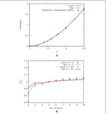
J-integral is a crucial parameter in our work because both the crack propagation and crack kinking criterion are entirely based on this single parameter. In order to study the accuracy ofJ-integral evaluation, we consider an edge crack specimen under simple extension. A 2 mm×2 mm plate withμs=0.4425 MPa and the equivalent Poisson ratio in the linear regimeν= 0.49 is taken, and the crack occupies half-width of the specimen. The strain energy function and boundary conditions are same as that of the previous example. These details are taken from an XFEM study [31], which reports the value ofJ-integral for large stretch ratios (λ).λis defined as the ratio of deformed length to the original length. We intentionally chose [31] as the reference for our validation because comparingJ-integral values at highλcould be challenging.

0 0.5 1 1.5 2

1 1.5 2 2.5

J

-in

tegral

λ

coarse fine Rashetnia, Mohammadi (2015)

a

0.7 0.8 0_.9 1 1.1 1.2 1.3

2 3 4 5 6 7 8 9 10

J

Jre

f

No. of layers

coarse_λ= 2

fine_λ= 2

coarseλ= 2.5 fineλ= 2.5

b

Fig. 7 Computation ofJ-integral:aVariation with respect to_λ.bDomain independency

mesh is only 1.3%. At the sameλ, the difference between the value reported in [31] and the present simulation using the fine mesh is as low as 3.4%. This quantitative comparison shows that theJ-integrals computed in our work are very accurate even at largeλ.

The variation ofJwith respect to the number of layers chosen around the crack tip as the integration domain is given in Fig.7b. It can be seen that after initial changes, the value ofJ is stable after 5 layers, after which only minute variations exist inJ. In all the simulations presented in this work, 5 layers of elements around the crack tip are chosen to compute theJ-integral.

Having simulated a stationary crack, the remaining examples consider complex crack propagation through the structure. The comparison between the present results and the results obtained from the literature demonstrates the accuracy of the method. For all the following examples, the strain energy function is given by Eq.4.

Single edge cracked plate under mixed-mode loading

7 7.5 8 8.5 9

0 1 2 3 4 5 6

y

x

Present Phongthanapanich, Dechaumphai (2004) Rao, Rahman (2000)

a b

c

Fig. 8 Single edge crack plate under mixed mode loading:aGeometry, material parameters and loading conditions; all dimensions are in mm.bContours of displacement in vertical direction.cCrack tip trajectory

Lame parameters are set such thatE=30 MPa andν=0.25. The computational domain is discretized with 2736 elements with the whole area of crack propagation discretized with a fine mesh.

view of crack path is plotted in Fig.8c, and the result obtained from the present simulation is compared with two other studies: one utilizes a meshless method [53], and the other study is based on adaptive FEM [6]. It can be seen that the predicted crack tip trajectory matches very well with the results obtained from the other two studies.

Crack in a drilled plate

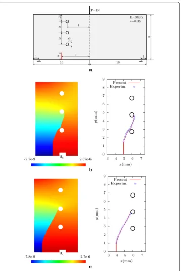
To demonstrate further the accuracy of the proposed method to simulate the crack path, the example given in [7] is considered. It reported the propagation of a crack from an initial notch in a beam which has three drilled holes. The study carried out both experimental and numerical tests, and observed a curvilinear crack propagation within the drilled plate. The geometrical configuration, material properties, and the loading conditions are given in Fig. 9a.The Lame parameters are set such thatE = 3 GPa and ν = 0.35. In this example, the stress/strain fields are influenced by the presence of holes in the beam, and this provides interesting curvilinear crack tip trajectories. There are two simulation cases considered based on the location of the initial notch. These are dictated by the choice of aandbin Fig.9a whose values are given in Table1for simulation-1 and simulation-2.

As reported in [7], the crack path follows different trajectories based on the choice ofa andb, which are described as follows.

Simulation-1

The location of the initial notch is given bya= 5 andb=1.5 mm. The crack is initially attracted towards the bottom hole, propagates near this hole, and got deflected away to end in the middle hole as shown in Fig.9b. This is in accordance with the experimental results of [7], and other numerical studies [3,6,54]. Comparison with the experimental results show that the present simulation produces very good results; even the crack deflection near the bottom hole is predicted well in the simulation as can be directly seen from Fig.9b. This is one of the very challenging validation test cases, owing to the complex crack tip trajectory involved. The developed methodology can be said to be accurate as it produces results that are matching very well with the experimental values even for this complex configuration.

Simulation-2

In this example, for whicha=6 andb=1 mm, the crack is attracted towards the middle hole, and directly ends in it (Fig.9c). There are no crack deflections observed, and for this example as well, the results match excellently with the experiment (Fig.9c).

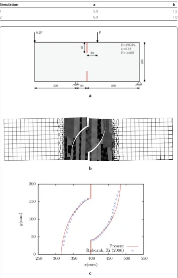
Four point beam with two notches

In order to test the performance of the present method to simulate multiple cracks in a structure, the four point bending beam with two pre-existing notches, shown in Fig.10a, is simulated. The beam is supported from below at two points, and is loaded at two other points. The material properties are also given in Fig. 10a. The computational domain is discretized with 7400 elements. This example is proposed by Bocca et. al. [55] who performed experiments on the structure, and also simulated them numerically.

Fig. 9 Bittencourt’s drilled plate problem.aGeometry,bSimulation-1,cSimulation-2. Experimental values for comparison are taken from [7]

Table 1 Geometric parameters defining notch location for Bittencourt’s drilled plate problem shown in Fig.9a

Simulation a b

1 5.0 1.5

2 6.0 1.0

40

P P

2 . 0

320 80 400

80

200

E=27GPa

ν=0.18 P=-100N

0 50 100 150 200

250 300 350 400 450 500 550

y

(mm)

x(mm)

Present Rabczuk, Zi (2006)

a

b

c

Though our method can handle multiple cracks, care must be taken to make sure that the domains used to evaluateJ-integral do not intersect with each other. However, this is not a specific drawback associated with our method alone. This is a common issue with other available approaches as well.

Crack deflection due to inclusion

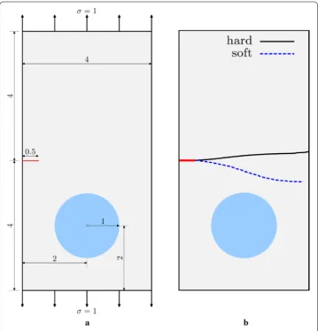
Crack growth in the presence of an inclusion is studied in this example. Geometry, loading, and boundary conditions are given in Fig.11a; they are taken from [57]. The configuration consists of a rectangular plate which contains an off-centre circular inclusion. The Lame parameters of the plate are set such thatE_plate=20 MPa andν=0.3. The objective of this study is to check whether the method is capable of accurately predicting the influence of this inclusion on crack propagation, which is already reported in [52,57].

The inclusion is characterized by the ratio of Young’s modulus of the plate to that of the inclusion (r=Eplate/Eincl.). Two values are considered;r=10 which means that the Young’s modulus of the inclusion is 10 times lower than that of the plate which is referred to as “soft” inclusion, andr=0.1 that is referred to as “hard” inclusion. The Poisson ratio

is assumed to be the same as that of the plate. The whole structural domain is discretized with 3213 elements.

The effect of the inclusion on the crack tip trajectory is shown in Fig.11b. For soft inclusion, the crack is attracted towards the side of the inclusion; however, the crack does not end in it. In case of a hard inclusion, the crack deflects away from it. These observations are consistent with the already reported results [52,57].

Nonlinear elastic plate with a hole

The above examples considered crack propagation with little material nonlinearity. This is evident from the fact that the crack remains sharp even after several propagation steps. The following example considers crack propagation involving high material nonlinearity under large deformation. A small off-centre hole is introduced in the geometric configuration considered for the first example, and this simulation allows the crack to propagate through the material. The Lame parameters are set to yieldE=10 GPa,ν=0.3; criticalJ-integral, Jc=50 kJm−2. The top surface is subjected to a displacement of 0.5 mm. The geometric configuration of this example is presented in Fig.12a.

As with the linear elastic examples, the loading (or the corresponding Dirichlet boundary condition here) is increased very smoothly from the zero initial value so that the influence of inertia is neglected. When the material starts deforming, as expected, the crack starts to blunt, and theJ-integral value starts to increase. WhenJ reaches Jc, then the crack starts to propagate; the deformed configuration of the structure at which the crack starts propagating is depicted in Fig.12b. Due to the presence of the hole, the crack slightly deflects upwards, as can be seen from Fig.12b, c. From all these plots, one can infer that the crack tip is always blunt owing to the material nonlinearity, and the present method is able to model fracture behavior in such scenarios.

Conclusion

A finite element methodology to model mixed-mode crack propagation through non-linear elastic materials is proposed in this work. The striking feature of this method is that it facilitates, with minimal implementation efforts, to update an existing large scale structural mechanics solver into a robust tool to handle single and multiple cracks. The method involves two steps: in the first step, the governing equations of the structure are solved using nonlinear FEM by freezing the crack in the structure; in the next step, the solution obtained from the FEM is used to propagate the crack based on the maximum energy release rate criterion. Advancing the crack through a FE mesh requires a continual change in topology of the mesh, which is achieved in this work by utilizing a mesh refit-ting approach. This method, as the name suggests, refits the mesh at each instant of crack advancement in such a way that the crack propagates through an existing edge in the mod-ified mesh. The mesh deformation strategies (for example used in ALE based methods) usually result in mesh tangling issues when attempting to handle topology changes in the mesh. This problem is circumvented in this work by splitting the quadrilateral elements into triangular elements in the crack tip neighborhood, which allows the possibility of local mesh connectivity to be modified. This step is crucial to preserve the quality of the mesh throughout the simulation, without which the mesh movement methods will fail. Examples involving single- and multi-materials with one or multiple cracks are reported. The obtained results are compared with experimental and other available computational methods. The comparison demonstrated that the present method accurately predicted the fracture behavior of all the examples considered.

Authors’ contributions

YS developed the idea, conducted numerical experiments and wrote draft. WAW fine-tuned the research idea, suggested numerical experiments and revised the paper. Both authors read and approved the final manuscript.

Competing interests

The authors declare that they have no competing interests.

Publisher’s Note

Springer Nature remains neutral with regard to jurisdictional claims in published maps and institutional affiliations.

Received: 30 August 2016 Accepted: 5 June 2017

References

1. Sudhakar Y, Wall WA. A strongly coupled partitioned approach for fluid-structure-fracture interaction. Int J Numer Methods Fluids; Submitted.

2. Wawrzynek PA, Ingraffea AR. An edge-based data structure for two-dimensional finite element analysis. Eng Comput. 1987;3:13–20.

3. Miehe C, Gürses E. A robust algorithm for configurational-force-driven brittle crack propagation with R-adaptive mesh alignment. Int J Numer Methods Eng. 2007;72:127–55.

4. Bouchard PO, Bay F, Chastel Y, Tovena I. Crack propagation modelling using an advanced remeshing technique. Comput Methods Appl Mech Eng. 2000;189:723–42.

5. Miranda ACO, Meggiolaro MA, Castro JTP, Martha LF, Bittencourt TN. Fatigue life and crack path predictions in generic 2D structural components. Eng Fract Mech. 2003;70:1259–79.

6. Phongthanapanich S, Dechaumphai P. Adaptive Delaunay triangulation with object-oriented programming for crack propagation analysis. Finite Elem Anal Design. 2004;40:1753–71.

7. Bittencourt TN, Wawrzynek PA, Ingraffea AR. Quasi-automatic simulation of crack propagation for 2D LEFM problems. Eng Fract Mech. 1996;55:321–34.

8. Camacho GT, Ortiz M. Computational modeling of impact damage in brittle materials. Int J Solids Struct. 1996;33:2899– 938.

9. Ortiz M, Pandolfi A. Finite-deformation irreversible cohesive elements for three-dimensional crack-propagation anal-ysis. Int J Numer Methods Eng. 1999;44:1267–82.

10. de Borst R. Numerical aspects of cohesive-zone models. Eng Fract Mech. 2003;70:1743–57.

12. Park K, Paulino GH. Cohesive Zone Models: a critical review of traction-separation relationships across fracture surfaces. Appl Mech Rev. 2013;64:060802.

13. Allix O, Ladevze P, Gilletta D, Ohayon R. A damage prediction method for composite structures. Int J Numer Methods Eng. 1989;27:271–83.

14. Genet M, Marcin L, Ladevze P. On structural computations until fracture based on an anisotropic and unilateral damage theory. Int J Damage Mech. 2014;23:483–506.

15. Celes W, Paulino GH, Espinha R. A compact adjacency-based topological data structure for finite element mesh representation. Int J Numer Methods Eng. 2005;64:1529–56.

16. Moës N, Dolbow J, Belytschko T. A finite element method for crack growth without remeshing. Int J Numer Methods Eng. 1999;46:131–50.

17. Sukumar N, Moës N, Moran B, Belytschko T. Extended finite element method for three-dimensional crack modelling. Int J Numer Methods Eng. 2000;48:1549–70.

18. Réthoré J, Gravouil A, Combescure A. An energy-conserving scheme for dynamic crack growth using the eXtended finite element method. Int J Numer Methods Eng. 2005;63:631–59.

19. Xiao QZ, Karihaloo BL. Improving the accuracy of XFEM crack tip fields using higher order quadrature and statistically admissible stress recovery. Int J Numer Methods Eng. 2006;66:1378–410.

20. Gupta V, Kim DJ, Duarte CA. Analysis and improvements of global-local enrichments for the generalized finite element method. Comput Methods Appl Mech Eng. 2012;245–256:47–62.

21. Gupta V, Duarte CA, Babuška I, Banerjee U. A stable and optimally convergent generalized FEM (SGFEM) for linear elastic fracture mechanics. Comput Methods Appl Mech Eng. 2013;266:23–39.

22. Nagarajan A, Mukherjee S. A mapping method for numerical evaluation of two-dimensional integrals with 1/r singularity. Comput Mech. 1993;12:19–26.

23. Béchet E, Minnebo H, Moës N, Burgardt B. Improved implementation and robustness study of the X-FEM for stress analysis around cracks. Int J Numer Methods Eng. 2005;64:1033–56.

24. Laborde P, Pommier J, Renard Y, Salaün M. High-order extended finite element method for cracked domains. Int J Numer Methods Eng. 2005;64:354–81.

25. Park K, Peraira JP, Duarte CA, Paulino GH. Integration of singular enrichment functions in the generalized/extended finite element method for three-dimensional problems. Int J Numer Methods Eng. 2009;78:1220–57.

26. Mousavi SE, Sukumar N. Generalized Duffy transformation for integrating vertex singularities. Comput Mech. 2010;45:127–40.

27. Mousavi SE, Sukumar N. Generalized Gaussian quadrature rules for discontinuities and crack singularities in the extended finite element method. Comput Methods Appl Mech Eng. 2010;199:3237–49.

28. Minnebo H. Three-dimensional integration strategies of singular functions introduced by the XFEM in the LEFM. Int J Numer Methods Eng. 2012;92:1117–38.

29. Dolbow J, Devan A. Enrichment of enhanced assumed strain approximations for representing strong discontinuities: addressing volumetric incompressibility and the discontinuous patch test. Int J Numer Methods Eng. 2004;59:47–67. 30. Legrain G, Moës N, Verron E. Stress analysis around crack tips in finite strain problems using the eXtended finite

element method. Int J Numer Methods Eng. 2005;63:290–314.

31. Rashetnia R, Mohammadi S. Finite strain fracture analysis using the extended finite element method with new set of enrichment functions. Int J Numer Methods Eng. 2015;102:1316–51.

32. Donea J, Huerta A, Ponthot JP, Rodrìguez-Ferran A. Arbitrary Lagrangian-Eulerian methods. In: Stein E, Borst R, Hughes TJR, editors. Encyclopedia of computational mechanics, vol. 1. Hoboken: Wiley; 2004.

33. Koh HM, Haber RB. A mixed Eulerian-Lagrangian model for the analysis of dynamic fracture. Illinois: Dept. of Civil Engineering, University of Illinois at Urbana-Champaign, Civil Engineering Studies, Structural Research Series; 1986. p. 524.

34. Koh HM, Lee HS, Haber RB. Dynamic crack propagation analysis using Eulerian-Lagrangian kinematic descriptions. Comput Mech. 1988;3:141–55.

35. Abdelgalil AI. Modeling of dynamic fracture problems using ALE finite element formulation. Vancouver: The University of British Columbia; 2002.http://hdl.handle.net/2429/13320.

36. Amini MR, Shahani AR. Finite element simulation of dynamic crack propagation process using an arbitrary Lagrangian Eulerian formulation. Fatigue Fract Eng Mater Struct. 2013;36:533–47.

37. Bruno D, Greco F, Lonetti P. A fracture-ALE formulation to predict dynamic debonding in FRP strengthened concrete beams. Compos Part B. 2013;46:46–60.

38. Ponthot JP, Belytschko T. Arbitrary Lagrangian-Eulerian formulation for element-free Galerkin method. Comput Meth-ods Appl Mech Eng. 1998;152:19–46.

39. Rashid MM. The arbitrary local mesh replacement method: an alternative to remeshing for crack propagation analysis. Comput Methods Appl Mech Eng. 1998;154:133–50.

40. Tabiei A, Wu J. Development of the DYNA3D simulation code with automated fracture procedure for brick elements. Int J Numer Methods Eng. 2003;57:1979–2006.

41. Browne PA, Budd CJ, Piccolo C, Cullen M. Fast three dimensional r-adaptive mesh redistribution. J Comput Phys. 2014;275:174–96.

42. Budd CJ, Russell RD, Walsh E. The geometry of r-adaptive meshes generated using optimal transport methods. J Comput Phys. 2015;282:113–37.

43. Belytschko T, Liu WK, Moran B. Nonlinear finite elements for continua and structures. Hoboken: Wiley; 2001. 44. Bonet J, Wood RD. Nonlinear continuum mechanics for finite element analysis. Cambridge: Cambridge University

Press; 1997.

45. Rice JR. A path independent integral and the approximate analysis of strain concentration by notches and cracks. J Appl Mech. 1968;35:379–86.

47. Shivakumar KN, Raju IS. An equivalent domain integral method for three-dimensional mixed-mode fracture problems. Eng Fract Mech. 1992;42:935–59.

48. Ma L, Korsunsky AM. On the use of vectorJ-integral in crack growth criteria for brittle solids. Int J Fract. 2005;133:L39–46. 49. Erdogan F, Sih GC. On the crack extension in plates under plane loading and transverse shear. J Basic Eng. 1963;85:519–

25.

50. Sih GC. Strain-energy-density factor applied to mixed-mode fracture problems. Int J Fract. 1974;10:305–21. 51. Hussain MA, Pu SL, Underwood JH. Strain energy release rate for a crack under combined mode I and mode II. Fract

Anal ASTM STP. 1974;560:2–28.

52. Bouchard PO, Bay F, Chastel Y. Numerical modelling of crack propagation: automatic remeshing and comparison of different criteria. Comput Methods Appl Mech Eng. 2003;192:3887–908.

53. Rao BN, Rahman S. An efficient meshless method for fracture analysis of cracks. Comput Mech. 2000;26:398–408. 54. Areias P, Dias-da-Costa D, Alfaiate J, Júlio E. Arbitrary bi-dimensional finite strain cohesive crack propagation. Comput

Mech. 2009;45:61–75.

55. Bocca P, Carpinteri A, Valente S. Mixed mode fracture of concrete. Int J Solids Struct. 1991;27:1139–53.

56. Rabczuk T, Zi G. A meshfree method based on the local partition of unity for cohesive cracks. Comput Mech. 2006;39:743–60.