STSMUS.pdf

State Taxes and Spatial Misallocation

∗

Pablo D. Fajgelbaum

UCLA& NBER

Eduardo Morales

Princeton & NBER

Juan Carlos Su´

arez Serrato

Duke & NBER

Owen Zidar

Princeton & NBER

August 2018

Abstract

We study state taxes as a potential source of spatial misallocation in the United States. We build a spatial general equilibrium framework that incorporates salient features of the U.S. state

tax system, and use changes in state tax rates between 1980 and 2010 to estimate the model

parameters that determine how worker and firm location respond to changes in state taxes.

We find that heterogeneity in state tax rates leads to aggregate welfare losses. In terms of consumption equivalent units, harmonizing state taxes increases worker welfare by 0.6 percent

if government spending is held constant, and by 1.2 percent if government spending responds

endogenously. Harmonization of state taxes within Census regions achieves most of these gains.

We also use our model to study the general equilibrium effects of recently implemented and proposed tax reforms.

∗

1

Introduction

Regional fiscal autonomy varies considerably across countries. In some countries, such as France,

Japan, and the United Kingdom, regional governments do not set tax policy. In others, such as

Germany, Italy, and Spain, regional governments have varying degrees of autonomy to set tax

rates, grant tax breaks, and introduce or abolish taxes. As a result, tax rates can vary considerably

across regions. Over time, several countries have adjusted their reliance on regional tax policies;

for example, Canada, Australia, and India have moved towards greater regional tax harmonization

in recent decades. The reasoning from recent research studying dispersion in distortions – across

firms, as in Restuccia and Rogerson (2008) and Hsieh and Klenow (2009), or across cities, as in

Desmet and Rossi-Hansberg (2013) – suggests that regional tax heterogeneity may have negative

aggregate effects by distorting the spatial allocation of resources. Early studies of local public

finance reinforce this logic by showing that, in some cases, allocative efficiency requires equal tax

payments across locations (Flatters et al., 1974; Helpman and Pines, 1980).

To the best of our knowledge, however, no quantitative evidence on the general equilibrium

tradeoffs between centralized and decentralized tax systems exists. We develop a spatial general

equilibrium model that incorporates salient features of the U.S. state tax code and quantify the

aggregate effects of dispersion in tax rates across U.S. states. The United States is a typical example

of a country with a decentralized tax structure, both in terms of the share of total tax revenue

collected by regional governments and the degree of spatial dispersion in tax rates.

In our model,

workers decide where to locate and how many hours to work based on each state’s taxes, wage,

cost of living, amenities, and availability of public goods, and firms decide where to locate, how

much to produce, and where to sell based on each state’s taxes, productivity, factor prices, market

potential (a measure of other states’ market sizes discounted by trade frictions), and provision of

public goods. We use the over 350 changes in state tax rates implemented between 1980 and 2010

to estimate the model parameters that determine how workers and firms reallocate in response to

changes in state taxes. Using the estimated model, we compute the general equilibrium effects

on worker welfare and aggregate income of replacing the current U.S. state tax distribution with

counterfactual distributions featuring varying degrees of dispersion in tax rates.

Overall, we find that tax dispersion leads to aggregate losses. In private consumption equivalent

units, harmonizing state taxes increases worker welfare by 0.6 percent if every state’s government

spending is kept constant. The gains to workers increase to 1.2 percent when we take into account

the impact that the change in taxes would have on each state’s government spending. Importantly,

most of these gains could be achieved by harmonizing taxes only across states located in the same

U.S. Census region. We also use our model to study the general equilibrium effects of recently

implemented and proposed state tax reforms, such as the limits to the State and Local Tax (SALT)

deduction imposed by the 2017 tax reform. We find that eliminating SALT increases tax dispersion,

1

results in welfare losses, and has heterogeneous effects across states depending on each state’s taxes,

income distribution, and composition of trading partners.

Our model embeds a canonical local public finance environment with many states, several fixed

(land and structures) and mobile (workers and firms) factors of production, and state governments

that use the tax revenue to finance the provision of public services which may be valued by workers

or used as intermediate goods in production. We generalize this framework in several directions.

First, we account for the main sources of tax revenue of U.S. state governments – sales, individual

income, and corporate income taxes apportioned through firm sales and factor usage – as well as for

federal taxes. Second, we allow states to have heterogeneous productivities, amenities, endowments

of fixed factors, and trade frictions with other regions; specifically, we model trade costs using the

standard approach in the quantitative trade literature (Eaton and Kortum, 2002; Anderson and

van Wincoop, 2003). Third, we assume that firms are monopolistically competitive, as in Dixit and

Stiglitz (1977) and Krugman (1980). Fourth, we allow workers’ preferences and firms’ productivities

to have idiosyncratic components that vary across states. These four ingredients allow our model

to match the observed responses of workers and firms to changes in taxes, and to rationalize as an

equilibrium outcome of our model the distribution of economic activity and trade flows observed

in any given year.

Our framework can be mapped to existing quantitative models of trade and economic geography.

We leverage properties of these models to implement counterfactuals with respect to the state tax

distribution, since a change to the tax distribution in our model is equivalent to a specific set

of changes in amenities, productivities, bilateral trade costs, and trade imbalances in a standard

trade and economic geography model such as Redding and Rossi-Hansberg (2017). Importantly,

determining this specific set of equivalent changes in fundamentals and trade imbalances requires

using the general equilibrium relationships predicted by our model to determine how much tax

bases change in the counterfactual.

We rely on a simpler version of our model to establish theoretically how worker welfare and

aggregate output depend on features of the U.S. state tax distribution. Eliminating dispersion in

state tax rates while keeping government spending constant may have a positive or negative effect

on worker welfare. As pointed out by Wildasin (1980), for any fixed arbitrary distribution of public

spending, efficiency requires equalization across states of tax payments per worker. The reason is

that efficiency requires equalization across locations of the marginal product of labor (which is equal

to the wage) net of the marginal social cost of attracting a worker to a location (which is equal

to consumption per capita). Absent compensating differentials (e.g., Hsieh and Klenow, 2009),

no dispersion in tax rates implies that tax payments are equalized. What is distinctive about a

spatial environment like ours is that wages and consumption per capita vary across locations due to

compensating differentials. Therefore, a change in tax rates may either increase or decrease

alloca-tive efficiency depending on its impact on the dispersion of tax payments per worker. Specifically,

eliminating dispersion in tax rates increases welfare if the cross-state correlation between tax rates

and fundamentals (productivity and amenities) is sufficiently large, since eliminating dispersion in

on real aggregate income is also theoretically ambiguous: eliminating tax dispersion may increase

or decrease aggregate real income depending on the initial correlation between state tax rates and

both state amenities and expenditure in public goods.

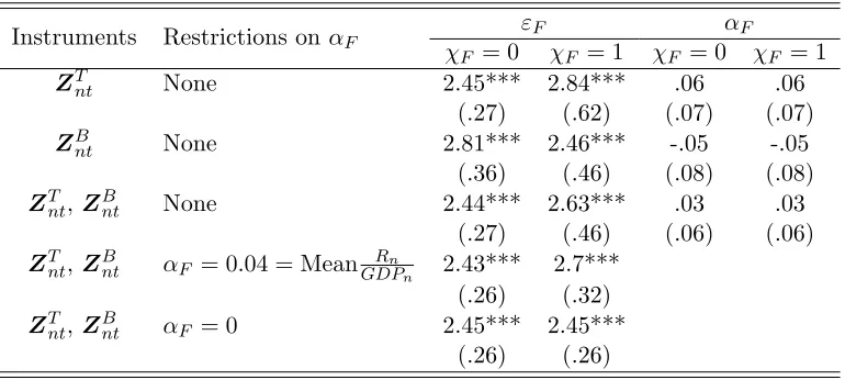
Four structural parameters are key for determining the impact of any change in taxes on worker

welfare and aggregate output: the elasticities of worker and firm mobility with respect to after-tax

real earnings and profits, respectively, and the weights that public services have in both workers’

preferences and firms’ productivity. To estimate these parameters, we use estimating equations

derived from our model and a longitudinal dataset containing each state’s number of workers and

establishments, tax rates, and government revenue between 1980 and 2010. Our model generates

a worker-location equation that models each state’s employment share as a function of that state’s

after-tax real earnings and government spending, and a firm-location equation that models each

state’s share of establishments as a function of that state’s after-tax market potential, factor prices,

and government spending. We then use observed worker and firm responses to actual changes in

taxes and state government spending to estimate the parameters entering these two equations. For

example, small estimated partial elasticities of employment shares and firm shares with respect

to government spending are rationalized in our model as a consequence of small weights of public

services in worker preferences and firm productivity, respectively.

Our estimation procedure uses several approaches to instrument for each state’s changes in

taxes, factor prices, and government spending. We instrument for these potentially endogenous

covariates using either taxes in other states or two Bartik-type instruments that exploit variation

in each state’s exposure to national industry shocks and national shocks that affect sources of tax

revenue differentially. This latter instrument exploits the fact that if, for example, a state’s tax

revenue comes mostly from sales taxes, then national sales booms will generate especially high

tax revenues for that state. Regardless of instrumentation strategy, the resulting estimates always

imply that workers’ and firms’ location decisions are more responsive to after-tax real wages or

profits, respectively, than to government spending. Our baseline estimates yield a partial elasticity

of state employment with respect to after-tax real wages of 1.1 and with respect to government

spending of 0.2, and a partial elasticity of the share of establishments in a state with respect to

after-tax market potential of 0.8 and with respect to government spending of 0.1.

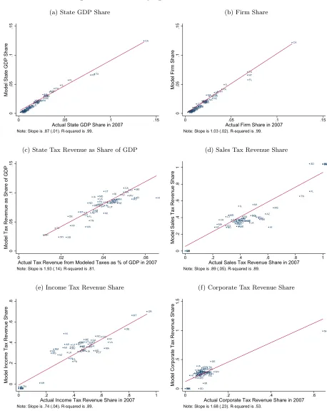
The outcomes of our counterfactuals also depend on state-specific production technologies,

productivities, amenities, and trade costs. These additional parameters are calibrated such that the

model exactly reproduces, as an equilibrium outcome, the distribution of labor and

intermediate-input income shares, wages, employment, trade flows, and trade imbalances across states observed

in 2007. We find that the distributions of states’ GDP and tax revenue shares in GDP implied by

the estimated model are very similar to those observed in the data, even though we do not use this

information to quantify the parameters of our model.

Using the estimated model, we implement a series of counterfactuals that demonstrate the

im-portance of state tax dispersion for aggregate outcomes in the U.S. From a theoretical perspective,

the question of how the distribution of state tax rates impacts the allocation of workers and firms

government spending impacts economic activity. Hence, when evaluating each counterfactual

dis-tribution of state taxes, we implement the analysis in two steps: first, holding the level of public

spending of every U.S. state constant at its initial level; and, second, allowing state spending to

change in response to the implied changes in tax revenue. The first step allows us to isolate the

impact of the tax distribution operating through spatial efficiency. The second step allows us to

take into account the impact of the tax distribution through changes in government spending.

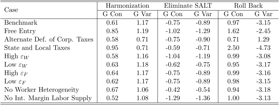
As mentioned above, we find that dispersion in U.S. tax rates across states leads to aggregate

welfare and output losses. These results are robust to alternative assumptions on how preferences

for government spending vary across states. In particular, they hold both in the extreme case in

which we assign zero weight to public services in workers’ preferences and firms’ productivity, and in

the case in which we assume that the observed ratio of government spending to GDP in each state

reflects its residents’ preferences for public services. These results are also robust to alternative

ways of measuring effective state tax rates; e.g., adjusting corporate tax rates for the share of

establishments in a state that are C-corporations, and adjusting income, sales, and corporate taxes

to account for local taxes.

We compute the aggregate implications of partial harmonizations that homogenize tax rates

only across subsets of states. We find that, as taxes are harmonized across a greater number of

U.S. states, the overall dispersion in tax payments per capita shrinks and, consequently, welfare

gains increase. Quantitively, however, we find that harmonizing taxes across states within the same

U.S. Census region generates welfare gains that are similar to those obtained under complete

har-monization. This regional harmonization result suggests that regional coordination of tax policies

could achieve most of the gains from harmonization across all U.S. states.

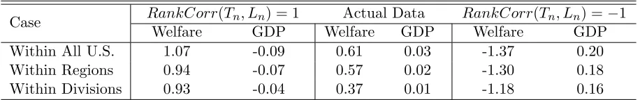
Our quantitative results show that the gains from tax harmonization would be different if the

distribution of fundamentals across U.S. states were different from that implied by the 2007 data.

Consistent with our theoretical analysis, a tax harmonization that keeps government spending

constant would lead to a larger increase in worker welfare if there were a higher correlation between

initial state tax rates and amenities or productivity. Therefore, the answer to the question of

whether a harmonized tax system that keeps government spending constant through a system of

transfers is superior to an alternative tax distribution that features dispersion in tax rates across

regions will depend both qualitatively and quantitatively on the specific country in question.

In terms of evaluating proposed tax reforms, we focus on the effects of eliminating the State and

Local Tax (SALT) deduction, which is one of the largest expenditures in the U.S. tax code and which

was substantially reduced by the Tax Cuts and Jobs Act of 2017. Eliminating SALT would increase

dispersion in tax payments, since places with high state taxes and high-income taxpayers would

pay even higher taxes. Consequently, we find that eliminating SALT reduces welfare by roughly

0.6 percent and aggregate real GDP by approximately 0.3 percent if government spending is held

constant, and by 0.8 and 0.4 percent, respectively, if government spending responds endogenously.

Southeastern states experience the largest gains. The hardest hit states are those with a large share

of high income people and high tax rates, especially in the Northeast. Cross-state trade linkages

enjoys the largest gains in real GDP despite having positive state income taxes, reflecting the

concentration of gains in nearby states. Similarly, among states with no state income tax, Florida

and Tennessee enjoy larger gains than states like Nevada, which is near states with high income

tax rates.

We also use our model to study the general equilibrium impact of actual tax reforms that have

taken place in the U.S. in recent years and of potential policy changes currently being discussed.

Over the past thirty years, U.S. state tax rates have increased on average, and they have become

more reliant on sales taxes. Overall, we find that these changes increased worker welfare and

aggregate output, and that these gains are driven in part by less dispersion in tax payments per

capita across states.

The rest of the paper is structured as follows.

Section 2 relates our work to the existing

literature. Section 3 describes features of the U.S. state tax system that motivate our analysis.

Section 4 introduces our model and describes its general equilibrium implications. Section 5 studies

theoretically how dispersion in taxes affects welfare and aggregate output in a simplified version

of our model. Section 6 presents our estimation approach, and Section 7 discusses our analysis

of counterfactual changes in taxes. Section 8 concludes. We provide additional derivations and

figures, and details on both our estimation approach and data sources in an Online Appendix.

2

Relation to the Literature

Misallocation

Our paper contributes to the literature on the aggregate effects of misallocation.

Distortions across firms are often measured as an implied wedge between an observed allocation

and a model-implied undistorted allocation, as in Hsieh and Klenow (2009). Recent papers have

adopted a similar methodology to analyze misallocation across geographic units, such as Desmet

and Rossi-Hansberg (2013), Brandt et al. (2013), and Behrens et al. (2017).

These wedges capture

distortions that may be due to multiple sources. Rather than inferring distortions from wedges,

we focus on quantifying the potential misallocation caused by dispersion in state taxes that we

directly observe in the data, and we use the observed variation in these taxes to estimate key model

parameters. Similarly, Albouy (2009) studies how federal tax progressivity impacts the allocation

of workers and aggregate outcomes.

Trade and Economic Geography

Our framework shares several components with recent

quan-titative economic geography models, such as Allen and Arkolakis (2014), Ramondo et al. (2016),

Redding (2015), and Caliendo et al. (2018). Our research question – the impact of state taxes on

the U.S. economy – drives our modeling choices, estimation approach, and counterfactuals. Relative

to this literature, we incorporate into our framework the main taxes imposed by U.S. states and

by the federal government as well as a government sector that uses tax revenue to finance public

services valued by workers and firms. Alongside workers with idiosyncratic preferences for location

as in Tabuchi and Thisse (2002) and others, we also introduce imperfect firm mobility through

firms that receive idiosyncratic productivity draws across states. A central feature of our analysis

is that we perform counterfactuals with respect to policy variables that are directly observed (U.S.

state tax rates) and use the observed variation in these same policies to identify the key model

parameters.

Fiscal Competition

The literature on fiscal competition, summarized among others by Oates

(1999) and Keen and Konrad (2013), typically considers static and perfectly competitive economies

with two or more regions and several factors of production, some of which are immobile and some

of which are mobile, which may be used to produce a consumption good and a non-traded public

good. These basic ingredients are included in our model. Our model generalizes this structure to a

multi-region setting in which the distribution of state characteristics can be disciplined using data

on the distribution of economic activity. A central question in this literature has been whether

jurisdictions setting tax policies according to the equilibrium of a non-cooperative game deliver a

socially efficient allocation. A recent quantitative study in the literature is Ossa (2018), who uses

an economic geography model with home-market effects to compute the Nash equilibrium of a game

where states use lump-sum taxes to finance firm subsidies. Our focus does not involve computing

the equilibrium of a non-cooperative game, so it does not require taking a stand on the objective

function or the information sets of policy makers, or on the process through which observed taxes

are determined.

Factor Mobility in Response to Tax Changes

We estimate elasticities of firm and worker

location with respect to taxes to identify key structural parameters. Evidence on the effect of

taxes on worker mobility includes Bartik (1991) and, more recently, Moretti and Wilson (2017).

Estimates of worker mobility across regions include Bound and Holzer (2000), Notowidigdo (2013),

and Diamond (2016). In terms of firm mobility, Holmes (1998) uses state borders to show that

manufacturing activity responds to business conditions, and a large literature studies the impact

of local policies on business location. Within this literature, Su´

arez Serrato and Zidar (2016)

provide evidence on the impact of corporate taxes on worker and firm mobility, Su´

arez Serrato

and Wingender (2016) show that local economic activity responds to public spending, and Giroud

and Rauh (2015) show that C-corporations reduce their activity when states increase corporate

tax rates.

Appendix D.9 compares our estimates to estimates from this prior literature. While

the aim of this literature is to quantify the local effects of actual policy changes, we use similar

empirical specifications and variation in the data to estimate key parameters of a general equilibrium

model, and then use these estimates to study how counterfactual policy changes in one state or

simultaneously in many states impact aggregate outcomes in the U.S. economy.

3

Background on the U.S. State Tax System

Our benchmark analysis focuses on three sources of state tax revenue: personal income taxes,

corporate income taxes, and sales taxes. The revenue raised through these three sources accounted,

respectively, for 35, 7, and 32 percent of total state tax revenue in 2007, and collectively amounted

to 4 percent of U.S. GDP.

In this section, we describe how we model each tax, present statistics

summarizing the dispersion in tax rates across states, and provide some evidence on how state

taxes relate to cross-state trade flows. Appendix F details the sources of the data we use.

3.1

Main State Taxes

Individual Income Tax

States tax the individual income of their residents. In 2007, the average

state income tax rate was 3.1%; the states with the highest average income tax rates were Oregon

(6.0%), North Carolina (5.0%), Minnesota (4.8%), and New York (4.8%), while seven states had

no income tax. State income tax rates tend to be progressive, but less so than federal income tax

rates. In our analysis, we approximate the schedule of income keep tax rates in each state, defined

as one minus the tax rate, through a log-linear function of income

y

: 1

−

t

(

y

) =

a

y

−byn,state

.

As Heathcote et al. (2017) recently argue, these functional forms accurately approximate U.S. tax

schedules. We compute the parameters of this tax schedule, (

a

, b

), for each state and

year using the average effective tax rate from NBER TAXSIM, which runs a fixed sample of tax

returns through each state’s income tax schedule every year and accounts for most features of the

tax code. Appendix Table A.3 reports the 2007 income tax schedule parameters.

Corporate Income Tax

States also tax businesses. The tax base and tax rate on businesses

depend on the legal form of the corporation. In our baseline analysis, we treat all businesses

4_{Additionally, Devereux and Griffith (1998) estimate the effect of profit taxes on the location of production} of U.S. multinationals, Goolsbee and Maydew (2000) estimate the effects of the labor apportionment of corporate income taxes on the location of manufacturing employment, Hines (1996) exploits foreign tax credit rules to show that investment responds to corporate tax regulations. Chirinko and Wilson (2008) and Wilson (2009) also provide evidence consistent with the view that state taxes affect the location of business activity.

5_{Our paper is also related to the literature that has analyzed the general equilibrium effects of tax changes.} Shoven and Whalley (1972) and Ballard et al. (1985) point out the importance of general equilibrium effects when analyzing large changes in policy. See Nechyba (1996) for an early Computable General Equilibrium (CGE) model of local public goods. A large literature in macroeconomics also studies the dynamic effects of taxes in the standard growth and real business cycle model; Mendoza and Tesar (1998), among others, study dynamic effects of taxes in an international setting.

6

as C-corporations — traditional corporations subject to the corporate income tax — since they

account for the majority of businesses’ net income in the United States.

In 2007, the average

state corporate income tax rate was 6.6%; the states with the highest corporate tax rates were

Iowa (12%), Pennsylvania (10%), and Minnesota (9.8%), while five states had no corporate tax.

State tax authorities determine the share of a C-corporation’s national profits allocated to their

state using apportionment rules, which aim to measure the corporation’s activity share in their

state. To determine this activity share, states put different weight on three apportionment factors:

the share of the corporation’s national payroll, property value, and sales. Payroll and property

factors thus depend on where goods are produced and typically coincide; the sales factor depends

on where goods are sold.

Apportionment through sales tends to be more prevalent: thirteen states

exclusively apportion through sales, while roughly three quarters of the remaining states apply

either a 50 or 33 percent apportionment through sales.

Sales Tax

Sales taxes are usually paid by the consumer upon final sale, and states typically do

not levy sales taxes on firms for purchases of intermediate inputs or goods that they will resell. In

2007, the average statutory general sales tax rate was 4.9%; the states with the highest sales tax

rates were California (7.25%), Mississippi (7%), New Jersey (7%), Maryland (7%), and Tennessee

(7%), while five states had no sales taxes.

3.2

Stylized Facts on State Taxes

Panels (a) to (c) of Figure 1 show that tax rates and tax revenue vary considerably across states.

Panel (a) shows the 2007 distribution of sales, income, corporate, and sales-apportioned corporate

tax rates.

Corporate tax rates are the most dispersed; the 90-10 percentiles of the distributions of

general sales, average personal income, and corporate income tax rates are 6.8%-1.5%, 4.6%-0%,

and 9.2%-1.0%, respectively. For each type of tax, there are at least five states with 0% rates.

7_{C-corporations are incorporated and officially registered business entities whose owners enjoy limited liability.} The other main type of business entities are private “pass-through” businesses, which are taxed at the owner rather than the entity level, i.e., the income that these private businesses earn passes through to the owners, who pay personal income taxes on their share of the firm’s income. C-corporations accounted for 66% percent of total business receipts in 2007 (PERAB, 2010). In robustness checks, we also explore how our results change when we adjust state corporate tax rates for the fraction of C-corporations revenue in each state’s total business revenue.

8

For example, a single-plant firm j located in stateiwith sales sharesj_ni in each state npays a corporate tax rate oftj=tcorp_{f ed} +tl

i+

P

ns j nit

x

n, wheret corp

f ed is the federal tax rate,t x

n=θxntcorpn is the corporate tax apportioned

through sales in state n (wheretcorpn is the corporate tax rate of staten and θxn is its sales apportionment), and tl

i= (1−θxi)t corp

i is the corporate tax apportioned through property and payroll in statei.

9

The sales-apportioned corporate tax rate is the product of the sales apportionment factor and the corporate rate; i.e. txn=θ

x nt

corp

n (see footnote 8). Table A.2 in Appendix F.2 shows the state tax rates in 2007 in all 50 states.

Figure 1: Stylized Facts on State Taxes

(a) Distribution of Tax Rates Across States

0

.1

.2

.3

.4

Density

0 5 10

State Tax Rates in 2007

Sales Individual Income

Corporate Sales Apportioned Corporate

(b) Tax Revenue as Share of GDP Across States

0

.02

.04

.06

.08

State Tax Revenue as Share of GDP in 2007 _{NH AK TX WY SD DE NV MT CO} IL

WA FL ND TN AL IAMO OR LA OK PA OH MD VA GA MI VT NE IN SC UT AZ CT NC KY NM RI KS NY MA WI NJ MN CA WV ID MS AR ME HI

Income Sales Corporate

(c) State Tax Rate Progressivity

0

2

4

6

8

State Income Tax Rate in 2007

0 50 100 150 200

Adjusted Gross Income ($1000)

State Avg. Iowa Indiana

(d) Trade Shares and Tax Rates

-4.4

-4.3

-4.2

-4.1

Log Bilateral Trade Share

.01 .02 .03 .04 .05 .06

Destination Corporate Tax Rate Weighted by Sales Apportionment (i.e., tx

) Note: Slope is -1.44 (.85). Controls for destination GSP. Includes origin, destination, and year FE.

Notes: Panel (a) shows the density of tax rates across states in 2007. Specifically, sales (tcn) and corporate income

(tcorpn ) tax rates are statutory, while individual income tax rates (tyn) are estimated using NBER’s tax simulator

TAXSIM. For each state, we compute average state tax liabilities and divide them by average Adjusted Gross Income (AGI) in that state. Finally, we compute sales apportioned corporate income tax rates (txn) by multiplyingtcorpn by

sales apportionment weights. Panel (b) shows state government tax revenue as a share of state GDP. Individual income, corporate income, and general sales tax revenues are drawn from Census Government Finances. Panel (c) shows how average state income tax rates in 2007 vary with taxpayer AGI for each state. For each level of AGI, we compute each state’s tax rate as tyn,state = 1−a

y n,statey

−by_n,state

. Progressivity is heterogeneous across states. For instance, the effective tax rate in Indiana is higher than Iowa for AGI below $30K, while the opposite is true for AGI above $30K. Panel (d) shows the OLS estimate of the coefficient from a regression of intra-U.S. trade flows on state corporate tax rates. Specifically, we compute bilateral trade shares as sin = Pxin

ixin, wherexin denotes sales

from state n to state i, and sales-apportioned corporate tax rates (txi) in destination states. The panel includes

These differences in tax structures across states are associated with differences in the total tax

revenue collected. Panel (b) shows the distribution of tax revenue as a share of state GDP by type

of tax. The share of the sum of income, general sales, and corporate tax revenue in GDP varies

across states between 1.1% and 6.5%. Local (sub-state) governments also tax residents. State taxes

amount to roughly 65% of state and local tax revenue combined.

Panel (c) plots our estimated

individual income tax schedules for all states in 2007. Some states like Indiana have flatter average

tax rates as a function of income, whereas others like Iowa have substantially more progressive

tax rates. Finally, panel (d) shows that inter-state exports are lower to destinations with high

sales-apportioned corporate taxes (see Table A.4 in Appendix A for additional evidence), after

controlling for state and year fixed effects.

3.3

State Tax Revenue and Government Spending

Besides taxes, transfers from the federal government are a major source of revenue for U.S.

state governments. On average across states, these transfers amounted to roughly 3.3% of their

GDP in 2007. Once these federal government transfers are taken into account, state governments

typically have balanced budgets (Poterba, 1994). Federal transfers therefore allow state spending

to exceed state tax revenue. The actual process determining these transfers is complex. However,

empirically, for the period 1980 to 2010, the size of the total direct expenditures of each state is

well approximated by a state-specific multiplier of that state’s tax revenue. Letting

R

be state

n

’s tax revenue and

E

= (1 +

ψ

)

R

be state

n

’s direct expenditures in year

t

, of which

ψ

R

is the part financed through federal transfers, the estimates of the regression

ln

E

= ln (1 +

ψ

) + ln

R

+

ε

(1)

yield an

R

of 0.97.

We adopt this relationship when modeling federal transfers in our quantitative

model.

4

Economic Geography Model with State Taxes and Public Goods

We model a closed economy with

N

states indexed by

n

or

i

. A mass of workers, normalized

to be of measure one, receives idiosyncratic preference shocks, which impact how they sort across

states. After the location decision has been made, each worker receives a productivity draw and

chooses how many hours to work. In our baseline model, a fixed mass of firms, also normalized to

be of measure one, sorts across states according, in part, to idiosyncratic productivity draws. For

10

Heterogeneity in tax rates across states is also present when both state and local taxes are taken into account. Figure A.1 in Appendix A reproduces panel (a) of Figure 1 using the sum of state and local tax rates. It shows that cross-state differences in tax rates increase when local tax rates are taken into account. Local governments rely mostly on property taxes. State tax revenue make up roughly 92%, 87%, and 79% of consolidated state and local revenue from income, corporate, and sales taxes, respectively, but only 3% of consolidated property tax revenue.

11_{We measure the variableE}G

ntusing “state direct expenditures” from the Census of Governments. The main

direct-expenditure items include: education, public welfare, hospitals, highways, police, correction, natural resources, parks and recreation, government administration, and utility expenditure. Panel (a) of Appendix Figure A.2 illustrates the close relationship betweenEG

robustness, we also examine an alternative model in which firms freely enter each location subject

to entry costs. We let

L

and

M

be the measure of workers and firms that locate in state

n

.

Each state

n

has an endowment

H

of fixed factors of production (land and structures), an

amenity level

u

, and a productivity level

z

.

There is an iceberg cost

τ

≥

1 of shipping from

state

i

to state

n

(if one unit is shipped from

i

to

n

, 1

/τ

units arrive). Firms are single-plant and

sell differentiated products. They use the fixed factor, workers, and intermediate inputs to produce

output. Workers only receive labor income, which they spend in the state where they live. Firms

and fixed factors are owned by immobile capital owners exogenously distributed across states.

State governments collect personal income taxes

t

(

y

) that depend on individual income

y

,

sales taxes

t

, and corporate income taxes apportioned through sales,

t

, and through payroll and

property,

t

. Each state uses the tax revenue to finance the provision of public services, which

enter as shifters of both that state’s amenity and productivity. The sensitivity of a state’s amenity

to public services may vary across states.

The federal government collects personal income taxes

t

(

y

), payroll taxes

t

, and corporate

taxes

t

. Federal taxes are used to finance federal transfers to state governments as well as federal

public goods that benefit any worker independently of their location (e.g., national defense).

4.1

Workers

A continuum of workers

l

∈

[0

,

1] decides in which state to work and consume. Each worker

l

observes a vector

of idiosyncratic state-specific preferences and decides the state of

resi-dence. Then, the worker discovers her own productivity level

z

in that state. This productivity

draw captures heterogeneity in job opportunities and gives rise to a non-degenerate income

distri-bution within each state. After observing her productivity in state

n

, each worker

l

chooses her

number of working hours,

h

. The total income of a worker

l

in state

n

is thus

w

h

z

, where

w

is the wage per efficiency unit and

h

n

z

are the efficiency units that worker

l

supplies in that state.

Workers have preferences over amenities, public goods, and final consumption goods, and

ex-perience disutility from working.

The direct utility of a worker who lives in state

n

, consumes

c

units of the private good, and works

h

hours is

U

(

c

, h

), where

U

(

c, h

) =

u

g

n

c

d

(

h

)

.

(2)

The amenity level

u

captures both natural characteristics, like the weather, and the rate at which

the government transforms total real spending into services valued by workers; this rate includes

the fraction of the state budget used to finance public services valued by workers. It may also

capture utility from a national public good provided by the federal government. The parameter

α

captures the weight of state-provided services in preferences. This weight may vary across

states, reflecting complementarities between state-specific features such as the weather or natural

amenities and government services. In turn, real government spending enjoyed by each worker

in state

n

,

g

, equals total real government spending,

G

, normalized by a function of the total

number of workers living in state

n

,

L

n

:

g

=

G

L

n

.

(3)

The parameter

χ

captures the degree to which public goods are rival, and ranges from

χ

= 0

(non-rival) to

χ

= 1 (rival). Workers also face disutility from effort, captured by the term

d

(

h

).

This disutility function is allowed to vary by state in order to give the model enough flexibility to

match cross-state differences in the per-worker number of hours worked. The indirect utility of a

worker

l

living in state

n

is

v

, where

v

≡

E

max

h

U

(

c

(

w

hz

)

, h

)

(4)

is the expected value over the possible realizations of the individual productivity shock

z

in state

n

, and where

c

(

y

) is the quantity of final goods consumed by an individual with income

y

in state

n

. We refer to

v

as the “appeal” of state

n

.

From the consumer’s budget constraint, and letting

P

be the price of the final good in state

n

, the final good consumption of an individual with income

y

living in state

n

is

c

(

y

) =

1

−

T

(

y

)

P

y,

(5)

where the real keep-tax rate is

1

−

T

(

y

)

≡

(1

−

t

(

y

))(1

−

t

(

y

))

1 +

t

.

(6)

This formulation takes into account that state income taxes can be deducted from federal taxes.

The idiosyncratic taste draw

is assumed to be independent and identically distributed

across individuals

l

and states

n

.

Hence, the fraction of workers located in state

n

is

L

=

Pr

n

= arg max

v

.

Assuming that the idiosyncratic taste draws follow a Fr´

echet

distri-bution, Pr(

< x

) = exp(

−

x

) with

ε

W

>

1, then

L

=

v

v

,

(7)

where

v

≡

X

n

v

n

!

.

(8)

The ex-ante expected utility of a worker over the distribution of taste draws

{

}

n=1

is proportional

to

v

. A larger value of

ε

implies that idiosyncratic taste draws are less dispersed across states; as

a result, locations become closer substitutes and an increase in the relative appeal of a location (an

We make additional functional-form assumptions to reach a closed-form solution for

v

. First,

we assume log-linear keep-tax schedules at the state and federal levels: 1

−

t

(

y

) =

a

y

−by_n,state

and 1

−

t

(

y

) =

a

y

f ed

.

These schedules are progressive (regressive) when the coefficients

b

and

b

adopt positive (negative) values. Together with (6), these forms imply

1

−

T

(

y

) =

a

y

y n

1 +

t

,

(9)

where

a

≡

a

a

,

(10)

b

≡

b

+

b

−

b

b

.

(11)

Second, we assume disutility from hours worked of the form

d

(

h

) = exp

−

α

h

1 + 1

/η

!

.

(12)

Together with (4), this functional form implies that utility is separable between consumption and

leisure and, thus, all workers in a state

n

work the same number of hours:

h

=

1

−

α

α

(1

−

b

)

.

(13)

Finally, we assume that productivity draws across workers located in state

n

follow a Pareto

dis-tribution with scale and shape parameters (

z

, ζ

):

Pr

h

z

≤

Z

i

= 1

−

Z

z

.

(14)

This assumption leads to the empirically consistent prediction of a fat-tailed income distribution.

The expressions (9) to (14) imply the following solution for the common component of utility

defined in (4):

v

=

ζ

ζ

−

(1

−

b

) (1

−

α

)

u

g

n

a

(1 +

t

)

P

w

z

h

e

y

n

.

(15)

Equation (15) captures several forces determining workers’ location. The first term reflects wage

heterogeneity within the state. Wage heterogeneity vanishes as

ζ

→ ∞

, in which case the individual

productivity distribution converges to a mass point at

z

. The average returns to locating in state

n

are also a function of the common component of amenities, public spending per capita, after-tax

wages and hours worked.

From the definitions of

L

and

v

in (7) and (15), the partial elasticity of the share of workers

while

ε

α

is the partial elasticity with respect to real government services per worker,

g

. We

will rely on these relationships to estimate

ε

and

{

α

}

in Section 6.2.

4.2

Capital Owners

Immobile capital owners located in state

n

own a fraction

ω

of a portfolio that includes the

profits of all firms in the economy and the payments to all fixed factors. In our model, a larger

ownership rate relative to other states results in larger trade imbalances. Therefore, we will calibrate

the ownership shares

ω

to match the observed trade imbalances across states.

Capital owners

spend their income locally, pay sales taxes on consumption, and pay the highest marginal rate for

both federal and state income taxes (Cooper et al., 2016). We do not need to specify the number

of capital owners or their utility function at any stage of our analysis.

4.3

Final Good

In each state, a competitive sector assembles a final good from differentiated varieties through

a constant elasticity of substitution aggregator with elasticity

σ

,

Q

=

X

i

Z

j∈Ji

q

σ

dj

!

σ−1

,

(16)

where

J

denotes the set of varieties produced in state

i

and

q

is the quantity of variety

j

produced

in state

i

which is used for production of the final good in state

n

. Letting

p

be the price of this

variety in state

n

, the cost of producing one unit of the final good in state

n

(and also its price

before sales taxes) is

P

=

X

i

Z

j∈Ji

p

dj

!

.

(17)

The final good

Q

is non-traded and can be used by consumers (workers and capital-owners) for

aggregate consumption of workers and capital owners (

C

and

C

), by firms as an intermediate

input in production (

I

), and by state governments (

G

) and the federal government (

G

) as an

input for the supply of public services:

Q

=

C

+

C

+

I

+

G

+

G

.

(18)

4.4

Firms

In our baseline model, we assume that there exists a fixed mass of firms which must decide in

which state to locate.

Assuming that these firms heterogeneous in terms of their productivity

across locations, this approach enables us to use data on firms’ location choices to estimate a

13_{Two alternative modeling approaches would be to assume that all workers own equal shares of the national} portfolio, or that the returns of that portfolio are spent outside of the model. Under these approaches, the model would lead to empirically inconsistent predictions for trade imbalances across states.

parameter determining the elasticity of the number of firms located in a state with respect to its

taxes. In this approach, taxes do not affect the mass of firms in the economy. To account for this

possible effect of taxes, we also explore the implications of an alternative model that features free

entry of firms with homogeneous productivity to each location, as in Krugman (1991) and Helpman

(1998). We describe the main implications of this alternative model at the end of this section.

Production Technologies

Each firm

j

∈

[0

,

1] produces a differentiated variety and is endowed

with state-specific productivities

{

z

}

i=1

. To produce quantity

q

j

i

in region

i

, firm

j

combines its

own productivity in that location

z

, a fixed factor

h

, efficiency units of labor

l

, and intermediate

inputs

i

, through a Cobb-Douglas technology:

q

=

z

"

1

γ

h

β

l

1

−

β

#

i

1

−

γ

,

(19)

where

γ

is the value-added share in production and 1

−

β

is the labor share in value added. The

fixed factor acts as a source of congestion: the higher the number of firms and workers located in

a given state, the higher the relative price of this fixed factor.

Profit Maximization given Firm Location

Each firm decides in which state to produce and

how much to sell in every state. Firms are monopolistically competitive. Consider a firm

j

located

in state

i

whose productivity is

z

. Its profits are

π

(

z

) = max

{

}

1

−

t

X

n=1

x

−

c

z

N

X

n=1

τ

q

!

,

(20)

where

t

is the corporate tax rate of firm

j

if it were to locate in state

i

,

x

=

P

Q

1

σ

n

(

q

)

−1

σ

are

its sales to state

n

, and

c

=

1 +

t

w

r

P

(21)

is the the minimum unit cost of a bundle of factors and intermediate inputs, where

w

is the wage

per efficiency unit,

r

stands for the cost of a unit of land and structures in state

i

and

t

are

federal payroll taxes. This definition of

c

accounts for the fact that, unlike consumers, firms do

not face sales taxes when purchasing the final good to use it as an intermediate.

All firms face corporate taxes apportioned through sales, payroll, and land and structures. A

firm

j

located in state

i

whose share of sales to state

n

is

s

pays a share

s

t

of its pre-tax

national profits in corporate taxes to state

n

. Firms located in

i

also pay a fraction

t

of its pre-tax

national profits in corporate taxes to state

i

, and a rate

t

in federal corporate income taxes. As

a result, the overall corporate tax rate of firm

j

is:

t

=

t

+

t

+

N

X

n=1

t

s

.

(22)

is not separable across states. When a firm increases the fraction of its sales to state

n

(i.e.,

when

s

increases), the average tax rate on the firm’s national profits changes depending on the

sales-apportioned corporate tax in state

n

,

t

. Firms thus trade off the marginal pre-tax benefit of

exporting more to a given state against the potential marginal cost of increasing the corporate tax

rate on all its profits.

Pricing Distortion Through Corporate Taxes

Despite the non-separability of the sales

deci-sion across markets, the solution to the firm optimization problem in (20) retains convenient

aggre-gation properties inherited from the standard CES maximization problem with constant marginal

production costs in Krugman (1980) or Melitz (2003). We describe these properties here and refer

to Appendix B.1 for details. Specifically, all firms located in a state

i

choose the same sales shares

across destinations irrespective of their productivity; i.e.,

s

=

s

for all firms

j

located in

i

. From

(22), this property leads to a common corporate tax rate across firms,

t

=

t

. Additionally, firms

set identical, constant markups over marginal costs, but these markups vary bilaterally depending

on corporate taxes. The price set in

n

by a firm with productivity

z

located in state

i

is:

p

(

z

) =

τ

σ

σ

−

˜

t

σ

σ

−

1

c

z

,

(23)

where

˜

t

≡

t

−

P

n0

t

s

1

−

¯

t

.

(24)

The term ˜

t

is a pricing distortion due to heterogeneity across states in the sales-apportioned

corpo-rate tax corpo-rates. This distortion increases with the sales tax in the importing state,

t

, implying that

prices will be higher in states with higher sales-apportioned corporate taxes.

If sales-apportioned

corporate tax rates were common across all states (

t

=

t

for all

n

, and, thus ˜

t

= 0 for all

i

and

n

), firms’ prices would be as predicted in the standard CES framework; i.e., the markup over

marginal cost would equal

σ/

(

σ

−

1).

Firm Location Choice

We assume that firm-level productivity

z

can be decomposed into a

term

z

common to all firms located in

i

and a firm- and state-specific component

, i.e.,

z

=

z

.

The common component of productivity is assumed to be:

z

=

G

M

i

z

i

.

(25)

This common component has an endogenous part that depends on the amount of public spending

and an exogenous part,

z

. The endogenous part equals total real government spending,

G

, divided

by a function of the number of firms located in state

i

,

M

i

, where the parameter

χ

captures

rivalry among the mass of firms

M

in the access to public goods. The exogenous part captures

natural characteristics that impact productivity, like natural resource availability, the rate at which

15

the government transforms real spending into services valued by firms, and the share of public

goods provided by state governments that increase the productivity of the firms located in their

states. Firm

j

decides to locate in state

i

if

i

= arg max

π

(

z

i0

). The idiosyncratic component

of productivity,

, is independent and identically distributed across firms and states and is drawn

from a Fr´

echet distribution, Pr(

< x

) = exp(

−

x

). As a result, the profits of firm

j

when

it locates in state

i

,

π

(

z

) =

π

(

z

)(

i

)

, are also Fr´

echet-distributed with shape parameter

ε

/

(

σ

−

1)

>

1. The fraction of firms located in state

i

is thus

M

=

π

z

¯

π

!

,

(26)

where

π

(

z

) is defined in (20) and ¯

π

is proportional to the expected profits before drawing the

idiosyncratic productivity shocks

{

}

i=1

. Equation (26) indicates that the fraction of firms located

in

n

depends on the common component of profits in

n

,

π

(

z

), relative to that in other locations.

A larger value of

ε

/

(

σ

−

1) implies that the idiosyncratic productivity draws are less dispersed

across states; as a result, states become closer substitutes and an increase in the relative profitability

of a state leads to a larger response in the fraction of firms that choose to locate in it.

Equilibrium State Productivity Distribution and Aggregation

As firms choose where to

locate based on their state-specific productivity draws, the productivity distribution in each state

is endogenous. State-level outcomes can be formulated as a function of a single moment ˜

z

of the

productivity distribution in each state

i

:

˜

z

=

z

M

− 1

εF

i

.

(27)

The productivity of the representative state-

i

firm, ˜

z

, is larger than the unconditional average of the

distribution of productivity draws (i.e., ˜

z

> z

), reflecting selection. This equation describes one of

the congestion forces in the model: as firms are heterogeneous and self-select based on productivity,

a higher number of firms locating in a state

i

is associated with lower average productivity in that

state.

Aggregate outcomes in state

i

can be constructed as if all of the

M

firms located there had

the (endogenous) productivity level ˜

z

. Appendix B.2 presents the expressions for the state-level

outcomes needed to compute the general equilibrium of the model.

Alternative Model with Free Entry of Firms

For robustness, we also perform counterfactuals

under the alternative assumption of free entry in each state

i

of firms with a common productivity

level

z

defined in (25). Conditional on entering state

i,

firms solve the problem (20) for

z

=

z

,

leading also to (22) to (24). To enter state

i

, firms must pay a cost equal to

f

units of the

cost-minimizing bundle of factors and inputs

c

in (21). In this alternative model, the zero-profit

16

By definition, ˜zi= (R_j∈J

i(z

j i)

σ−1

dj)σ1−1_{. To reach (27), we use the equalityπ(˜zi) = ¯π(implied by the Fr´echet}

condition

π

(

z

) =

c

f

thus determines the number of firms in each state

i

. Appendix B.2

presents the expressions for the state-level outcomes needed to compute the general equilibrium of

the model under this free entry assumption. As in the baseline model, the number of firms in each

state turns out to also be proportional to aggregate sales in the state.

4.5

State Governments

State governments use state tax revenue

R

and transfers from the federal government

T

to finance spending in public services,

P

G

. The budget constraint of state

n

is thus

P

G

=

R

+

T

,

(28)

where the tax revenue collected by the state is

R

=

R

+

R

+

R

,

(29)

and where

R

,

R

, and

R

n

denote government revenue from corporate, sales, and income taxes,

respectively. These expressions are defined in (A.15) to (A.17) in Appendix B.2.

Consistent with the empirical evidence in Section 3.3, we assume that transfers from the federal

government to state governments are proportional to the tax revenue collected by these state

governments, where the constant of proportionality

ψ

may vary by state:

T

=

ψ

R

.

Combined with (28), this relationship implies that

P

G

= (1 +

ψ

)

R

. While the distribution of

federal transfer rules

{

ψ

}

impacts all model outcomes in levels, they do not have any impact

on the counterfactual results we report in Section 7.

4.6

Federal Government

The federal government uses income and corporate taxes to finance transfers to state

govern-ments and to purchase the final good produced in each state,

G

, which it employs as an input

in the production of a national public good. Our analysis assumes that public services from the

federal government are valued in the same way across locations.

4.7

General Equilibrium

A general equilibrium of this economy consists of distributions of workers and firms

{

L

, M

}

,

aggregate quantities

{

Q

, C

, C

, I

, G

, G

}

, wages per efficiency unit and cost of fixed

fac-tors

{

w

, r

}

, and final good prices

{

P

}

such that: i) final good producers optimize, setting

their prices according to (17); ii) workers make consumption, work hours and location decisions

optimally, as described in Section 4.1; iii) budget constraints of capital owners hold; iv) firms make

17_{Under free entry, the number of firms in state iis M}

i = (1−ti)Xi/(σcifE,i). Under a fixed mass of ex-ante

heterogeneous firms, Mi = (1−ti)Xi/(σπ¯).The free-entry model has thus an additional parameter per state, the

entry cost fE,i, which can be calibrated to exactly match the observed number of firms per state. However, as

production, sales, and location decisions optimally, as described in Section 4.4; v) government

bud-get constraints hold, as described in Section 4.5; vi) final good markets clear in every location, i.e.,

(18) holds for all

n

; vii) the labor market clears in every state, i.e., labor supply (7) equals labor

demand (given by (A.7) in Appendix B.2) for all

n

; viii) the land market clears in every state, i.e.,

(A.8) in Appendix B.2 holds; and ix) the national labor market clears, i.e.,

P

n

L

= 1.

4.8

Adjusted Fundamentals and Implementation of Counterfactuals

According to our model, taxes in any state may affect outcomes in every state. However, as

shown in Appendix B.3, state tax rates

t

, t

(

·

)

, t

, t

n=1

only impact state outcomes through

their effect on a set of

adjusted fundamentals

,

{{

τ

}

i=1

, z

, u

}

,

z

=

1

−

¯

t

σ

−

1

1

εF+αFχF

G

n

z

−αF

n

,

(30)

τ

=

σ

σ

−

˜

t

τ

,

(31)

u

=

1

−

T

z

L n

w

1 +

t

!

G

n

u

,

(32)

and on the set of relative trade imbalances

{

P

Q

/X

}

(i.e., the ratio between state

expen-ditures and sales). Adjusted fundamentals (

z

, τ

, u

) become identical to state fundamentals

(productivity

z

, amenity

u

, and trade costs

τ

) if we assume away preferences for government

spending (

α

=

α

= 0) and set all tax rates to zero.

In our model, the distribution of outcomes across states depends on the distributions of adjusted

fundamentals and relative trade imbalances similarly to how it depends on the state fundamentals

and relative trade imbalances in standard economic geography models such as Allen et al. (2014) or

Redding (2015). Therefore, the effect of a counterfactual change in the tax distribution predicted

by our model is identical to the effect of a specific set of changes in amenities, productivities, trade

costs, and trade imbalances in a standard economic-geography model. Importantly, the mapping

from taxes to adjusted fundamentals and relative trade imbalances depends on the specific features

of the tax system that we incorporate in our framework. Thus, to compute our model-predicted

impact of counterfactual changes in the tax distribution, we simultaneously use a mapping from

changes in fundamentals to changes in outcomes that is standard in existing economic-geography

models, as well as a mapping from changes in taxes to changes in adjusted fundamentals that is

specific to our environment. The first mapping is presented in (A.35) to (A.42) in Appendix B.5,

and the second one in (A.43) to (A.46).

4.9

Agglomeration and Congestion Forces

Our model features agglomeration forces that push workers and firms to locate in the same state,

as well as congestion forces that push them to spread across different states. Specifically, our model

(who consume final goods) and firms (which purchase intermediate inputs) have an incentive to

locate near or in states with low price indices and large markets; in turn, the price index of a state

decreases with the number of firms located in that state, and its market size increases with the

number of workers located in it. Our model also features agglomeration through public service

provision as long as public goods are not fully rival (i.e., as long as either

χ

or

χ

are less than

one). States with a larger number of firms and workers have higher tax revenue and public spending

and, thus, higher utility per worker (see (4)) and firm productivity (see (25)).

At the same time, our baseline model features congestion through immobile factors in

produc-tion, leading to a higher marginal production cost in a state as employment increases in that state

(see (A.8) in Appendix B.2); through selection of heterogeneous firms, leading to a lower average

firm productivity in a state as the number of firms increases (see (27)); and through the presence

of immobile capital owners, who spend their income where they are located.