The Joint Effect of Firing Costs
on Employment and Productivity
in Search and Matching Models
Bj¨orn Br¨
ugemann
∗October 2006
Abstract
In the textbook search and matching model the effect of firing costs on employment is generally ambiguous as both accessions and separations are reduced. Similarly, the effect on average productivity of matches is ambiguous as less productive matches survive while hiring becomes more selective. Thus it would seem that the theory does not generate predictions with respect to the effect of firing costs on employment and productivity. In this paper I show that the theory does generate predictions about the jointresponse of employment and productivity: while employment may increase or average productivity may rise, it is not possible that both occurs together. That is, firing costs must have a negative effect on at least one of the two outcomes employment and average productivity.
Keywords: Employment Protection, Firing Costs, Employment, Productivity. JEL Classification: E24, J63, J65
∗Department of Economics, Yale University, 28 Hillhouse Avenue, CT 06511. E-mail:
Much research on employment protection policies has focussed on effects of such policies
on the level of employment. Theoretical work has not delivered general predictions on the
sign of this effect. In some models employment protection reduces separations and thereby
increases employment, in others it reduces hiring and thereby reduces employment, or both
effects may be present, making the overall effect ambiguous. Thus the direction of the effect
is generally regarded as something to be ascertained empirically. A large number of empirical
studies have attacked this question using a variety of approaches, and while the balance points
to a negative effect, the evidence is far from overwhelming.1
Establishing empirically the impact of firing costs on productivity is even more
challeng-ing and has only been attempted in a recent paper by Autor, Kerr, and Kugler (2006). They
preface their analysis stressing that in theory the sign of this effect is also ambiguous:
em-ployment protection may reduce productivity by inducing firms to retain some unproductive
worker, but this is potentially offset by firms screening new hires more stringently.
The Mortensen-Pissarides search and matching model is one of the most commonly
em-ployed theoretical frameworks for studying the effects of firing costs and labor market policies
more generally. Within this framework both ambiguities discussed above arise. An increase
in firing costs in general reduces both hiring and separations, making the employment effect
ambiguous; less productive matches survive while hiring becomes more selective, leading to
an ambiguous effect on employment.
Thus it would seem that theory makes no predictions regarding the effect of firing costs on
employment and productivity, and that this statement also applies to the specific environment
of the Mortensen-Pissarides search and matching model. In this paper I show that it is
not quite true that this model makes no predictions about the response of employment and
productivity to an increase in firing costs. While it is true that it makes no predictions about
how the two variables respond individually, the model does restrict their joint behavior in
response to an increase in firing costs. I show that while employment may increase or average
productivity may rise, it is not possible that both occurs together.
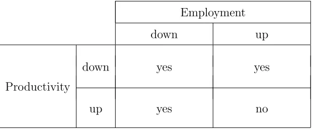
Table 1 displays the possible joint responses of employment and productivity to an increase
in firing costs. After describing the search and matching model in section 1, in section 3 I show
by example that the model can generate each joint outcome indicated affirmatively in Table
1
Employment
down up
down yes yes
Productivity
up yes no
Table 1: Possible Effects of Firing Cost.
1. Section 4 contains the main theoretical result of the paper, namely that the outcome in the
lower right corner of Table 1 is impossible: an increase in firing cost cannot simultaneously
increase employment and productivity. Specifically, I will show that if an increase in firing
costs increases employment, then it must shift down the distribution of productivity among
employed workers in the sense of first order stochastic dominance. Section 5 concludes.
1
Search and Matching Model with Firing Costs
Time is discrete. There is a continuum of infinitely lived ex ante identical workers of mass
one. At a point in time a worker is either employed or unemployed. The production structure
of the economy consists of many firm-worker matches, each composed of one worker and one
firm.
Timeline. The timing of events within a period is as follows. At the beginning of the
period a fraction of workers in existing matches quits exogenously. Then surviving matches
receive a new draw of match specific productivity. Next workers unemployed at the end of
last period and vacancies posted during last period are matched and each new match receives
an initial draw of match specific productivity. This is followed by separation decisions in all
matches. Now production takes place in surviving matches. Finally firms decide whether to
post vacancies.
Preferences. All agents have linear utility with discount factor (1−ρ)∈(0,1): the utility
of a consumption streamCt is given by P
∞
Creation. Maintaining an open vacancy is associated with a cost c per period. If at the
end of this period the number of unemployed workers is uand the number of open vacancies
isv, then the number of new matches created next period is given by m(u, v). The matching
functionmhas constant returns to scale, is continuous, strictly increasing in both arguments,
and satisfies m(u, v) < min{u, v}. An open vacancy is matched with probability q(θ) ≡
m 1θ,1
. The matching probability of an unemployed worker is f(θ) ≡ m(1, θ). The ratio
θ = v
u is referred to as labor market tightness. To insure existence of equilibrium I assume
that limθ→∞q(θ) = 0.
Production. The initial productivity of a new match is drawn from a distribution given
by the distribution functionG0. Subsequently a match experiences idiosyncratic productivity
shocks. In particular, match specific productivity follows a Markov process with state space
Y and transition function Q. The process is stochastically monotone: if productivity is
high today, it is likely to be high tomorrow; formally y′ ≥ y implies that Q(y′,·) first order
stochastically dominates Q(y,·). In addition, I make two standard technical assumptions.
First, I assume that the state space is a bounded interval Y = [ymin, ymax]. Second, I assume
that the transition function satisfies the Feller property.2 The payoff of non-market activity
received by unemployed workers is denoted as z ≥0.
Destruction. There is both exogenous and endogenous destruction. At the beginning of
each period a match is destroyed exogenously with probability ˜δ ∈(0,1). Idiosyncratic shocks
to match specific productivity are the source of endogenous destruction.
Employment Protection. When dismissing a worker, the firm is bound by statutory
em-ployment protection, which is modeled as wasteful firing costs F ∈ F ⊆R+. After meeting a
worker firms can decide not to form a match and walk away without paying the firing costs.
Bargaining. For illustrative purposes I will follow the bulk of the literature and use the
standard assumption that separations are bilaterally efficient and that at the time of creation
the worker and the firm split the value of the match via Nash bargaining with shares β and
1−β, respectively.
2
The Markov process has the Feller property ifR
f(z′)Q(z, dz′) is a bounded and continuous function ofz
I emphasize, however, that the specific model of wage determination does not play an
important role in the results. I will point out those implications of Nash bargaining that the
results do rely on.
2
Steady State Equilibrium
2.1
Partial Equilibrium Separation and Match Formation Decision
In steady state equilibrium the utility of unemployed workers U is constant. In this section
I will study the partial equilibrium separation and creation decision taking as given a level
of unemployed utility. In section 2.2 I turn to the determination of the utility of unemployed
workers in general equilibrium.
In order to study the separation decision, consider a match that has already been created.
The separation decision is made to maximize the joint value of the match. Let V∗(y, U, F)
be the joint value of a match with productivity y in an environment with firing costs F and
constant utility of the unemployedU. It solves the equation
V∗(y, F, U) = max
y+δU + (1−ρ−δ)
Z
V∗(y′, F, U)Q(y, dy′), U −F
. (1)
where I defineδ≡(1−ρ)˜δ for notational convenience. The second argument of the maximum
operator is the joint payoff if the match dissolves today, given by the utility of unemployment
obtained by the worker minus the firing cost liability of the firm. The first argument of the
maximum operator is the value of continuing the match. This yields output y this period.
With probability ˜δ the match separates exogenously in which case the firm obtains zero (it
does not have to pay the firing cost) while the worker obtains the utility (1−ρ)U. Taken
together this yields the present discounted joint payoff δU. If the worker does not quit the
match survives into the next period, receives a new productivity drawy′, and once again faces
the same decision.
The following lemma establishes the properties of the value function V∗ relevant for the
analysis here. All proofs not given in the text are collected in the appendix.
Lemma 1. (a) There exists a unique threshold y(F, U) ∈ R such that V∗(y, F, U) equals
U −F for y ≤ y(F, U) and is strictly increasing in y for y ≥ y(F, U). The threshold
(b) Consider FH > FL. The difference V(y, FH, U)−V(y, FL, U) is non-positive. It is
bounded below by FL−FH.
(c) Consider UH > UL. The difference V(y, F, UH)−V(y, F, UL) is positive. It is bounded
above by UH −UL, strictly so if y > y(F, UH).
Part (a) implies that separation occurs if productivity drops strictly below a threshold
productivity level y(F, U). If productivity equals y(F, U) the match is indifferent between
separation and continuation. For simplicity I assume that the match continues in this
situ-ation. Higher firing costs make splitting up less attractive, while less painful unemployment
hastens separations. Part (b) considers the comparative statics of the joint value with respect
to firing costs. An increase in firing costs reduces the value of the match, but by less than the
increase in firing costs as the latter are incurred at some point in the future. Similarly, part
(c) establishes that an increase in the utility from unemployment increases the joint value,
but not by more than the increase in the utility from unemployment.
Next I discuss how the joint value of the match is split between the worker and the firm, and
the decision whether or not a match is formed. First suppose that a match with productivity
y is formed. Then the worker and the firm share the value of the match via Nash bargaining
W(y, F, U)≡U +β[V∗(y, F, U)−U],
J(y, F, U)≡(1−β) [V∗(y, F, U)−U].
(2)
HereW(y, F, U) is the utility of the worker andJ(y, F, U) is the value of the firm. The outside
opportunity of the worker is unemployed utility U. At the time of match creation the firm
can still walk away without paying the firing cost, so its outside opportunity is zero. Thus
the surplus of the match is V∗
(y, F, U)−U, and each of the two parties receives its outside
option plus a share of the surplus.
Next consider the match formation decision. It is clear from equation (2) that both parties
are willing to form the match if the surplus V∗(y, F, U)−U is non-negative. Since the joint
value is increasing iny it follows that the match is formed if productivity exceeds a threshold
y0(F, U) implicitly defined by the equation
V∗(y0(F, U), F, U) =U. (3)
For convenience I assume that a match is formed if the surplus is exactly zero. The match
Lemma 2. (a) Positive firing costs F >0 imply y0(F, U)> y(F, U).
(b) The threshold y
0(F, U) is weakly increasing in F and strictly increasing in U.
Proof. It follows from property (a) of Lemma 1 that the separation threshold satisfies
V∗(y(F, U), F, U) = U − F. This implies V∗(y(F, U), F, U) < V∗(y
0(F, U), F, U). Since
V∗(y, F, U) is strictly increasing in y for y ≥ y(F) it follows that y
0(F, U) > y(F, U). This
proves part (a). Turning to part (b), first consider an increase in firing costsF. This weakly
reduces the left hand side of equation (3) andy0(F, U) must increase weakly to restore equality.
For an increase inU property (b) of Lemma 1 implies that the right hand side of (3) increases
more than the left hand side, soy0(F, U) must increase strictly to restore equality.
Property (a) states that as long as firing costs are positive the hiring threshold is more stringent
than the separation threshold. This is due to the assumption that at the time of match
formation the worker and the firm can still walk away without being subject to firing costs.
According to property (b) an increase in firing costs for given utility of the unemployed
leads to stricter hiring standards. This is because an increase in firing costs reduces the value
of the match. An increase in the utility of the unemployed increases the opportunity cost
of forming a match more than it increases the value of a match, so again hiring standards
become more stringent.
Define the ex ante value of the match as
V0∗(F, U)≡
Z ymax
y0(F,U)
V∗(y, F, U)dG0(y). (4)
It is easy to check that it inherits the comparative statics properties of the joint value V∗
established in parts (b) and (c) of Lemma 1.3 The ex ante payoff of the firm and the worker
are
W0(F, U)≡U +β[V0∗(F, U)−U],
J0(F, U)≡(1−β) [V0∗(F, U)−U].
(5)
3
The last statement in part (b) is not directly applicable to V∗
0; V0∗(F, UH)−V0∗(F, UH) is strictly less
thanUH−UL as long as 1−G
2.2
General Equilibrium
In a steady state equilibrium the utility of the unemployed U and labor market tightness θ
must satisfy the following two conditions.
c≥(1−ρ)q(θ)J0(F, U) with equality if θ >0, (6)
ρU =z+ (1−ρ)f(θ) [W0(F, U)−U]. (7)
Condition (6) is the free entry condition for posting vacancies. The left hand side is the return
from posting a vacancy, that is the present discounted value of being matched with a worker
next period. In equilibrium it cannot exceed the vacancy cost c and must equal this cost if
any vacancies are posted. Condition (7) states that the flow value of unemploymentρU is the
sum of the value of non-market activity z and the capital gain from being matched with an
employer in the next period.
The following lemma establishes existence and uniqueness of the steady state values of
labor market tightnessθ and unemployed utility U, and how they vary with firing costs F.
Lemma 3. (a) (Existence and Uniqueness) For each level of firing costs F ∈ F the
condi-tions (6)–(7) have a unique solution (Uss(F), θss(F)).
(b) (Comparative Statics) Both Uss(F) and θss(F) are weakly decreasing in F.
Proof. See Appendix B for the proof of part (a). Turning to part (b), first consider the
utility of unemployed workers. Suppose that unemployed utility increases in response to an
increase in firing costs. Then by equation (6) labor market tightness must fall, since both the
increase in firing costs and the increase in the utility of the unemployed reduce the value to
the firm of meeting a worker. This drop in labor market tightness reduces the probability
that an unemployed worker finds a job. Moreover, both the increase in F and the increase
in U reduce the capital gain from finding a job. Thus the right hand side of equation (7)
falls, contradicting the increase in U. Labor market tightness must also fall. The only way
an increase in labor market tightness could be consistent with the entry condition (6) is for
J0(F, U) to increase. The sharing rule (5) then implies that W0(F, U) must increase as well.
The right hand side of (7) then increases both because of higher labor market tightness and a
higher capital gain from finding a job, contradicting the fall in the utility of the unemployed.
The separation and match formation thresholds as a function of firing costs are given by
yss(F)≡y(F, Uss(F)) andyss
0 (F)≡y0(F, U
ss(F)). It is clear that the steady state separation
threshold is strictly decreasing in firing costs F since both the direct and the indirect effect
work in the same direction. In contrast, the direct effect of higher employment protection
is to increase the match formation threshold, while the indirect effect through unemployed
utility is to lower this threshold. Thus in general the effect of an increase in firing costs on
the steady state match formation threshold is ambiguous.4
2.3
Productivity Distribution and Employment
Take a pair (y
0, y) consisting of a match formation threshold and a separation threshold.
The following lemma establishes that such a pair induces a unique steady distribution of
productivity among employed workers.
Lemma 4. If G0(y0−)<1a pair(y0, y)withy≤y0 induces a unique steady state distribution
of productivity among employed workers.
HereG0(y0−) is the lefthand limit of G0 aty0. The conditionG0(y0−)<1 implies that if
a worker and a firm meet they form a match with positive probability. IfG0(y0−) = 1 all new
matches have productivity strictly below y0, that is the hiring threshold is so stringent that
steady state employment is necessarily zero, in which case there is no meaningful distribution
of productivity across employed workers.
Let Gss
emp(·|y0, y) denote the unique steady state distribution of productivity among
em-ployed workers. Then the steady state destruction probability is given by
d(y
0, y)≡δ˜+
1−˜δ
Z
Q(y,[ymin, y))Gssemp(dy|y0, y).
The first term of the sum is the probability of exogenous destruction. The second term
captures endogenous destruction: a match with productivity y that has escaped exogenous
destruction is destroyed endogenously if its new productivity draw is below y, which occurs
with probabilityQ(y,[ymin, y)).
4
In fact, under the assumptions made here once can show that this threshold must be increasing in firing
costs. But this property may not generalize to other models of wage determination. Moreover, it is not needed
Steady state employment as a function of the two thresholds and labor market tightness
is given by
Lss(y0, y, θ)≡ f(θ)(1−G0(y0−))
f(θ)(1−G0(y0−)) +d(y0, y)
. (8)
With slight abuse of notation I write the productivity distribution and employment as a
function of firing costs as
Gssemp(·|F)≡Gssemp·|yss
0 (F), y ss
(F),
Lss(F)≡Lssyss0 (F), yss(F), θss(F).
3
Possible Joint Responses
In this section I begin the analysis of the joint response of employment and productivity to an
increase in firing costs. I provide an example for each joint outcome indicated affirmatively
in Table 1. This sets the stage for the next section where I show that the only joint outcome
that is not possible is for both employment and productivity to increase.
3.1
Employment Up and Productivity Down
A special case of the model in which employment increases while productivity declines is
obtained by imposing two restrictions on the general model. First, I shut down the hiring
margin by letting the initial productivity distribution G0 be degenerate, so all matches start
at a common productivity levely0. Second, since in general an increase in firing costs reduces
recruiting effort of firms, I minimize the negative impact this has on employment by assuming
that this recruiting effort plays no productive role in matching, that is m(u, v) = ˜µu for
˜
µ∈ (0,1). In this case, as long as matches with productivity y0 are formed, the job finding
rate is constant at µ and not negatively affected by increases in firing costs. It then follows
that an increase in firing costs only reduces job destruction, thereby increasing employment.
As hiring does not become more selective while destruction is delayed, it also follows that the
productivity distribution shifts down.
As an illustration, consider the following simple productivity process which I will utilize
again to construct the other examples in this section. All matches start with productivity y0,
level of firing costs, one in which low productivity matches are destroyed and one in which
they survive.
First I compute the value of a new match under the assumption that low productivity
matches are destroyed. Later I will check when this is correct. One obtains
V∗(y0, F, U) =y0+δU + (1−ρ−δ) [˜γ(U −F) + (1−γ˜)V∗(y0, F, U)].
Solving forV∗(y
0, F, U) yields
V∗
(y0, F, U) =
y0 −γF + (δ+γ)U
ρ+δ+γ . (9)
where I define γ ≡ (1− ρ−δ)˜γ for notational convenience. Substituting into equilibrium
condition (7) gives
ρU =z+µβy0−γF −ρU ρ+δ+γ .
Solving forρU yields
ρU = (ρ+δ+γ)z+µβ(y0−γF)
ρ+δ+γ +µβ . (10)
The assumption that low productivity matches are destroyed is correct if
y1+δU
ρ+δ < U −F. (11)
The left hand side is the value of continuing in the low productivity state, the right hand
side is the value of termination. Substituting forU from equation (10), this condition can be
written as an upper bound on the low productivity level:
y1 <
(ρ+δ+γ)z+µβy0
ρ+δ+γ+µβ −
(ρ+δ+µβ)(ρ+δ+γ)
ρ+δ+γ+µβ F. (12)
Now I choose productivity parameters in the following way. First I sety0 > z and then I pick
y1 ∈
(ρ+δ+γ)z+µβy0 ρ+δ+γ+µβ , y0
. Let F1 be the level of firing costs for which (12) holds with equality.
The restrictions on the productivity levels insure that F1 > 0. Now consider an increase in
firing costs from zero to F1. Steady state employment levels are given by Lss(0) = δ+µγ+µ
and Lss(F1) = δ+µµ. Thus this increase in firing costs strictly increases employment. At zero
firing costs all matches have high productivity, while atF1 only a fraction γ+γδ do. Thus this
increase in firing costs is associated with a downward shift of the productivity distribution in
3.2
Employment and Productivity Down
In the preceding example I eliminated the negative effect of firing costs on employment by
making recruiting effort of firms irrelevant for match creation. In this example I want
em-ployment to be decreasing, so I go to the opposite extreme and assume that only vacancies
enter the matching function, i.e. m(u, v) = ˜µv.
Again I start by solving for the equilibrium assuming that low productivity matches are
destroyed. Equation (9) for the value of a high productivity match still applies, but now I
need to substitute this value into the entry condition (6) in order to obtain an equation for
unemployed utilityU:
c=µ(1−β)y0−γF −ρU
ρ+δ+γ .
Solving forρU yields
ρU =y0−γF −
(ρ+δ+γ)
µ(1−β) c. (13)
Labor market tightness is obtained by substituting the utility of the unemployed into condition
(7):
θss(F) = max
1
βµ
(1−β)µy0−z−γF
c −(ρ+δ+γ)
,0
(14)
which is valid as long as the assumption of low productivity matches being destroyed is correct.
Now given the parametersρ,δ,γ,β,candµI picky0 ∈
ρ+δ+γ ρ+δ z+
(ρ+δ+γ)c (1−β)µ ,
ρ+δ+γ ρ z+
(ρ+δ+γ)c (1−β)µ
and set y1 = 0. The lower bound on y0 insures that that labor market tightness is strictly
positive at zero firing costs.
As before the assumption that low productivity matches are destroyed is correct if
inequal-ity (11) holds. Substituting from equation (13) into this inequalinequal-ity yields the following upper
bound on the low productivity level:
y1 < y0−(ρ+δ+γ)
c
µ(1−β) +F
. (15)
LetF1 be the level of firing costs such that inequality (15) holds with equality. It is
straight-forward to check that the restrictions ony0 along with y1 = 0 implies that F1 is positive.
Now consider an increase in firing costs from zero to F1. Again this turns a productivity
distribution with only high productivity matches into a distribution in which a fraction γ+γδ
of matches has low productivity.
substi-tuting into equation (14) yields
θss(F1) = (
1
βµ
"
(1−β)µ
(ρ+δ)y0+γy1 ρ+δ+γ −z
c −(ρ+δ)
#
,0
)
.
The lower bound on y0 along with y1 = 0 insures that θss(F1) is strictly positive. Since
Lss(0) = µθss
(0)
µθss(0)+δ+γ while L ss(F
1) = µθ
ss
(F1)
µθss(F1)+δ it follows that employment falls if θ ss(F
1) < δ
δ+γθ
ss(0). It is straightforward to verify that the upper bound on y
0 insures that this is
satisfied.
3.3
Employment Down and Productivity Up
In the preceding examples I considered increases in firing costs that did not make firms more
selective in hiring because all matches started at the same level of productivity y0. Now I
assume that initial productivity can take two levels,yH
0 with probabilityφ and y0L< yH0 with
probability 1−φ, letting y0 denote mean initial productivity y0 = φy0H + (1−φ)y0L. From
both levels of initial productivity, a drop to productivity y1 ≤ y0L occurs with probability
˜
γ. Additionally, I return to the assumption that firm recruiting effort is irrelevant for the
production of matches, that is m(u, v) = ˜µu. Thus firing costs do not affect labor market
tightness. As a consequence an increase in firing costs can reduce employment only by making
firms sufficiently more selective in hiring. This will be the case in this example.
Suppose matches with low initial productivity are formed. Then it is easy to verify that
the utility of the unemployed is once again given by equation (10). The value of a match with
low initial productivity is
V∗(y0L, F, U) = y
L
0 −γF + (δ+γ)U
ρ+δ+γ .
For the assumption that matches with low initial productivity are formed to be correct it
must be thatV∗(yL
0, F, U)≥U. This yields the condition
yL0 ≥ (ρ+δ+γ)(z+γF) +µβφy H 0
ρ+δ+γ+φµβ
LetF0L be the level of firing costs at which this condition is satisfied with equality. For firing
costs aboveFL
0 matches with low initial productivity are formed. As before letF1 be the level
of firing costs for which equation (12) holds with equality. Thus for firing cost levels strictly
Now pick productivity levels as follows. First chooseyH
0 > z, then sety0L=
(ρ+δ+γ)z+φµβyH 0 ρ+δ+γ+φµβ .
This insuresFL
0 = 0. Finally picky1 ∈
z,(ρ+ρ+δ+δ+γ)γz++µβµβy0. This insures F1 >0. Now consider
an increase in firing costs from zero to any level strictly belowF1. This increase is not enough
to keep matches with productivityy1 from being destroyed, but it keeps matches with initial
productivity yL
0 from being formed. Hence this increase in firing costs reduces employment
fromµ+µδ+γ to µφ+µφδ+γ. In addition, it turns a productivity distribution with a fraction (1−φ) of
matches with low initial productivityyL
0 into a productivity distribution in which all matches
have high initial productivityyH
0 . Thus employment falls while the distribution of productivity
among employed workers shifts up in the sense of first order stochastic dominance.
Remark. The example above demonstrates that it is not true in general that FH > FL
implies that for all productivity levels y∈ Y
1−Gssemp(y|FH)≤1−Gssemp(y|FL),
that is it is not true in general that the distribution of productivity across employed workers
shifts down in the sense of first order stochastic dominance. However, even if this distribution
shifts up, it could still be generally true that FH > FL implies
Lss(FH)
1−Gssemp(y|FH)
≤Lss(FL)
1−Gssemp(y|FL)
.
That is, while the number of workers with productivity abovey may increase as a fraction of
employed workers, it could still be the case that it must decrease as a fraction of all workers.
For this property to hold, the increase in unemployment must be sufficient to overturn any
upward shift in the productivity distribution. The example above has been constructed in
such a way that it also violates this weaker property: the increase in firing costs considered
in the example increases workers with high initial productivityyH
0 as a fraction of all workers
from µ+µφδ+γ to µφ+µφδ+γ.
4
Impossibility of Employment and Productivity Up
In this section I establish the main result of the paper: an increase in firing costs cannot both
increase employment and productivity. More precisely, I show that if an increase in firing
costs does not decrease employment, then it must be associated with a downward shift in the
So far I have proceeded under the standard assumption that wages are determined through
Nash bargaining. This particular assumption is not needed for the result of this section to
apply. What is needed is the following. Consider an increase in firing costs from FL ≥ 0 to
FH > FL. Let θH ≡θss(FH),θL≡θss(FL), yH ≡yss(FH),yL ≡yss(FL), yH 0 ≡y
ss 0 (F
H) and
yL0 ≡ yss0 (FL). Under Nash bargaining an increase in firing costs reduces both labor market
tightness and the separation threshold, that isθH ≤θL and yH ≤yL. In addition, for a given
level of firing costs the match formation threshold exceeds the separation threshold, that is
yL 0 ≥ y
L and yH 0 ≥ y
H. These implications of Nash bargaining are all that is needed, so the
result of this section will extend to an alternative model of wage determination as long as it
reproduces these implications.
So far nothing has been said about how the increase in firing costs affects the match
formation threshold. The case in which the match formation threshold falls along with the
separation threshold is easily dealt with: in this case the productivity distribution shifts down
irrespective of what happens to employment.
Lemma 5. Consider (yH0 , yH) with yH0 ≥ yH and (y0L, yL) with yL0 ≥ yL. If yH0 ≤ yL0 and
yH ≤yL, then Gss
emp(y|yH0 , yH)≥Gempss (y|yL0, yL) for all y∈ Y.
It remains to consider the case in which the match formation threshold increases. As
demonstrated in the last example of the previous section, in this case it is possible for the
productivity distribution to shift up. However, the following proposition establishes that this
is only possible if employment decreases. Let LH ≡Lss(FH) and LL≡Lss(FL).
Proposition 1. Consider (yH0 , yH, θH) with yH0 ≥ yH and (yL0, yL, θL) with yL0 ≥ yL. If
yH ≤yL, θH ≤θL, and LH ≥LL, then Gss
emp(y|yH0 , yH)≥Gempss (y|yL0, yL) for all y ∈ Y.
Proof. The case yH
0 ≤ y L
0 has been dealt with in Lemma 1. So suppose y H 0 > y
L 0. Let
¯
G0(y)≡1−G0(y) be the probability that a new matches has productivity strictly higher than
y. A quantity that will play an important role in the proof will be the steady steady inflow
into productivity levels strictly larger thany as a fraction of employment. It is given by5
m(y|y
0, y)≡
1−Lss(y0, y, θ)
Lss(y 0, y, θ)
f(θ) ¯G0(max{y0, y}). (16)
5
Although bothLss(y
0, y, θ) and f(θ) depend on θ, is is easy to check using the formula for steady state
Let ¯Gssemp(y|y0, y) ≡ 1−Gssemp(y|y0, y) be the fraction of workers with productivity strictly
abovey in steady state. Then for y∈[y, ymax]
¯
Gssemp(y|y
0, y) =m(y|y0, y)
+1−δ˜
Z ymax
ymin
Q(y′,(y, ymax])Gssemp(dy
′
|y0, y) +Q(ymin,(y, ymax])Gssemp(ymin|y0, y)
.
The left hand side is the fraction of employed workers with productivity above y at the time
of production this period. It is the sum of two terms. The first term is the mass of workers in
new matches with productivity above y as a fraction of employment. The second term is the
mass of old matches who survived exogenous destruction and received a productivity draw
abovey this period.6 Integration by parts yields
¯
Gssemp(y|y0, y)
=m(y|y
0, y)−
1−δ˜
Z ymax
ymin
Gssemp(y′|y
0, y)Q(dy
′
,(y, ymax]))−Q(ymax,(y, ymax]))
for y∈[y, ymax]. This can be rewritten as
¯
Gssemp(y|y
0, y)
=m(y|y0, y) +1−δ˜
Q(ymin,(y, ymax]) + Z ymax
ymin
¯
Gssemp(y
′
|y0, y)Q(dy′,(y,+∞))
(17)
fory∈[y, ymax]. This expression has the following interpretation. If the distributionGssempwere
degenerate with all mass at productivityymin, then exactly a fraction
1−δ˜Q(ymin,(y, ymax])
of matches would survive into next period with productivity above y. This is not the case
if not all mass is at ymin. In particular, matches with productivity above ymin have a higher
chance of survival, and the integralRymax ymin G¯
ss
emp(y′|y0, y)Q(dy′,(y, ymax])) accounts for this fact
by adding the increment in the survival chances for matches with productivity aboveymin.
Notice that yH0 > yL0 implies ¯G0(max{yH0 , y}) ≤ G¯0(max{yL0, y}) for all y ∈ Y. Using
equation (16), this fact along with the increase in employment and the decrease in labor
market tightness implies
m(y|yH
0 , y H
)≤m(y|yL
0, y L
)
for all productivity levels y∈ Y. The reason for this is straightforward. The high firing costs
economy has fewer unemployed workers who meet firms at a lower rate, so it is clear that
6
The contribution of workers with last period productivity at the lower bound ymin is not captured by
the integral and must be added separately. Of course this term is zero if there is no mass point at ymin, in
the mass of new matches above a certain level productivity levels is lower. Since employment
is higher in the high firing costs economy, this holds also when this mass is considered as a
fraction of employment.
Taking the difference of equation (17) with respect to the two levels of firing costs yields
¯
Gssemp(y|yH0 , yH)−G¯ssemp(y|yL0, yL) =m(y|yH0 , yH)−m(y|yL0, yL)
+1−δ˜
Z ymax
ymin h
¯
Gssemp(y′
|yH
0 , y H
)−G¯ssemp(y′
|yL
0, y L
)iQ(dy′,
(y, ymax])
(18)
for y ∈ [yL, ymax]. Now suppose the distribution under low firing costs does not
domi-nate the distribution under high firing costs. Then over some range the difference between ¯
Gssemp(y′|yH0 , yH) and ¯Gssemp(y′|yL0, yL) is positive. Thus the least upper bound of this gap is
strictly positive:
sup
y′∈Y
h
¯
Gssemp(y
′
|yH0 , yH)−G¯ssemp(y
′
|yL0, yL)i >0. (19)
Clearly
¯
Gssemp(y|y H 0 , y
H
)−G¯ssemp(y|y L 0, y
L
)
≤1−δ˜sup
y′∈Y
h
¯
Gssemp(y
′
|yH0 , yH)−G¯ssemp(y
′
|yL0, yL)i[Q(ymax,(y, ymax])−Q(ymin,(y, ymax])]
(20)
for y∈[y
L, ymax]. To interpret this inequality, notice that the second term on the right hand
side of equation (18) gives the contribution of the gaps last period to the gap at
produc-tivity level y this period: if the distribution under high firing costs has more mass above
y′ last period, it tends to have more mass above y this period. Under what circumstances
is this contribution as large as possible, taken as given the upper bound (19)? This occurs
if the gap is constant and equal to the upper bound for all y ∈ Y. This corresponds to
the extreme case in which last period the distribution with high firing costs is the same as
the distribution under low firing costs except for some mass shifted from ymin to ymax. This
maximizes the contribution of this term due to stochastic monotonicity: matches with
pro-ductivityymin this period are least likely to be aboveynext period, whereas this is most likely
for matches with productivity ymax this period. The difference in these probabilities is given
byQ(ymax,(y, ymax])−Q(ymin,(y, ymax]). This difference is at most one, which corresponds to
the extreme case in which matches with productivity ymax this period will be above y next
y next period. Thus
¯
Gempss (y|yH0 , yH)−G¯ssemp(y|yL0, yL)≤
1−δ˜sup
y′∈Y
h
¯
Gssemp(y
′
|yH0 , yH)−G¯ssemp(y
′
|yL0, yL)i (21)
for y ∈ [yL, ymax]. This immediately generates a contradiction: even when conditions last
period are most conducive to creating a gap this period, the gap next period cannot exceed a
fraction (1−δ˜)<1 of the least upper bound of the gap last period.7 Thus there cannot be a
gap in steady state, that is
sup
y′∈Y
h
¯
Gssemp(y′|yH
0 , y
H)−G¯ss emp(y
′
|yL
0, y
L)i ≤0
which implies
Gssemp(y′|yH0 , yH)≥Gssemp(y′|yL0, yL)
for all y∈ Y.
5
Concluding Remarks
I have shown that the standard search and matching model has a testable implication for
the joint behavior of steady state employment and productivity in response to an increase in
firing costs. A natural extension would be to analyze whether this holds not only in steady
state but also throughout the transition from the low firing costs steady state to the high
firing costs steady state, and the other way around. This stronger type of prediction would
be easier to test empirically.
7
We derived inequality (21) only for y ∈ [yL, ymax]. For y ∈ [ymin, y
L) it is necessarily true that ¯
Gss
emp(y|yH0 , y
H)−G¯ssemp(y|yL
0, y
L)≤0 since ¯Gssemp(y|yL
0, y
A
Proof of Lemma 1
In equilibrium utility from unemployment cannot be lower than the utility from perpetual
unemployment U≡ z
ρ. Boundedness of the state space Y implies that utility from
unemploy-ment cannot exceed some upper bound ¯U for any value of firing costsF. Thus it is sufficient to
analyze the separation decision for utility from unemployment varying in the setU ≡ [U,U¯].
Firing costs are allowed to vary inF =R+. I will establish a more comprehensive result from
which Lemma 1 immediately follows.
Lemma A. The joint value function V∗
is bounded, continuous, and has the following
prop-erties.
(a) For each (F, U)∈ F ×U there exists a unique thresholdy(F, U)∈Rsuch thatV∗(y, F, U)
equals U −F for y≤y(F, U) and is strictly increasing in y for y≥y(F, U).
(b) Fix U ∈ U. Consider FH, FL ∈ F with FH > FL. Then y(FH, U) < y(FL, U). The
difference V∗(y, FH, U)−V∗(y, FL, U) is non-positive and bounded below by FL−FH.
(c) Fix F ∈ F. Consider UH, UL ∈ U with UH > UL. Then y(F, UH) > y(F, UL). The
difference V∗(y, F, UH)−V∗(y, F, UL) is non-negative and bounded above by UH −UL,
strictly so for y > y(F, UH).
Proof. LetV′
be the set of functionsV :Y ×F ×U →Rsatisfying all the properties stated
in the lemma. LetV be the set of functions obtained when the strictly increasing requirement
in property (a) is replaced by weakly increasing, and the strict requirements in properties (b)
and (c) are replaced by the corresponding weak requirements. Define the operator
(T V)(y, F, U)≡max
y+δU + (1−ρ−δ)
Z
V(y′, F, U)Q(y, dy′), U −F
.
I will show thatT(V)⊆ V′. The desired result then follows from Corollary 1 to the Contraction
Mapping Theorem in Stokey and Lucas (1989) in conjunction with the fact thatVis a complete
metric space. To verify the claim thatT(V)⊆ V′, supposeV ∈ V. Then T V is bounded and
continuous by Lemma 9.5 in Stokey and Lucas. It remains to verify properties (a)–(c).
(a) Define
(CV)(y, F, U)≡y+δU + (1−ρ−δ)
Z
V(y′, F, U)Q(y, dy′).
As V is weakly increasing in y and Q is stochastically monotone, it follows that the
to the unique solution of the equation (CV)(y, F, U) =U −F. Then (T V)(y, F, U) =
U−F for y≤y(F, U) and (T V)(y, F, U) is strictly increasing in y for y≥y(F, U).
(b) ConsiderFH, FL ∈ F withFH > FL. Since 0≥V(y′, FH, U)−V(y′, FL, U)≥FL−FH
for ally′ ∈ Yit follows that 0≥(CV)(y, FH, U)−(CV)(y, FL, U)≥(1−ρ−δ)(FL−FH).
Since the value of separation drops by FH −FL it follows that 0 ≥ (T V)(y, FH, U)−
(T V)(y, FL, U) ≥ FL−FH. Next consider the comparative statics of the separation
threshold. As (CV)(y(FL, U), FL, U) = U−FLit follows that (CV)(y(FL, U), FH, U)>
U−FH, so it must be that y(FH, U)< y(FL, U).
(c) The proof of property (c) proceeds in exactly the same way as the proof of property (b).
To obtain the additional result that the upper boundUH−ULis strict fory≥y(F, UH),
notice that in this case
(T V)(y, F, UH)−(T V)(y, F, UL) = (CV)(y, F, UH)−(T C)(y, F, UL)
≤δ(UH −UL) + (1−ρ−δ)(UH −UL)< UH −UL.
B
Proof of Lemma 3
Proof of Lemma 3. First consider equation (7) for a given value ofθ. The left hand side
is strictly increasing in U while the right hand side is weakly decreasing in U. Both are
continuous in U.8 For U = z
ρ the right hand side exceeds the left hand side. Since the left
hand side is unbounded it follows that there is a unique solution ˆU(θ). The function ˆU is
continuous. Since an increase in θ strictly increases the right hand side of equation (7) it
follows that ˆU(θ) is strictly increasing. Substituting into the right hand side of equation (6)
yields the term (1−ρ)q(θ)J0(F,Uˆ(θ)), which is continuous and strictly decreasing in θ. If it is
strictly less thancforθ= 0, then the equilibrium has θss(F) = 0 andUss(F) = z
ρ. Otherwise
the assumption that limθ→∞q(θ) = 0 insures that there is a unique valueθss(F) for which this
term equals c. Equilibrium utility from unemployment is then given by Uss(F) = ˆU(θss(F)).
8
Proof of Lemma 4. In steady state the mass of workers separating equals the mass of
workers entering employment. Thus the distribution of productivity across employed workers
can be computed from the transition function induced by Q when separated matches are
replaced by matches with productivity drawn fromG0. This transition function is given by
Qemp(y, Y|y0, y)≡
1−δ˜Q(y, Y ∩[y, ymax])
+δ˜+1−δ˜Q(y,[ymin, y))
µ0(Y ∩[y
0, ymax])
µ0([y0, ymax])
.
where µ0 is the probability measure associated with the distribution function G0. The first
term of the sum is the probability of transiting to a productivity level in the setY by surviving
both quits and the separation decision at the beginning of next period. The second term of
the sum is the probability of transiting to the set Y via replacement through new matches
with a productivity level within that set. It is the product of the destruction rate and the
probability of new matches having productivity in Y. Notice that the latter probability is
conditional on a new match being formed. LetT∗
emp(·|y0, y) be the adjoint operator associated
with Qemp(·|y0, y) and let Temp∗n (·|y0, y) be the n-fold composition of this operator.9
To prove the lemma I will show that this transition function satisfies Condition M in
Stokey and Lucas (1989, page 348). Set ε = 1
4δ˜. Take any Y ∈ B where B is the σ
-algebra associated with the productivity state space Y. . First suppose µ0(Y∩[y0,ymax]) µ0([y0,ymax]) ≥
1 2.
Then Qemp(y, Y|y0, y) ≥ 12δ > ε˜ for all y ∈ Y. Next suppose
µ0(Y∩[y0,ymax]) µ0([y
0,ymax])
< 12. Then
µ0(Yc
∩[y 0,ymax]) µ0([y0,ymax]) >
1
2 and Qemp(y, Y c|y
0, y) > 1
2˜δ > ε for all y ∈ Y. Thus Condition M is
satisfied and Theorem 11.12 in Stokey and Lucas (1989, p. 350) implies thatT∗
emp(·|y0, y) has
a unique invariant measureµssemp(y0, y) and thatTemp∗n (µ|y0, y) converges strongly toµssemp(y0, y)
asn → ∞for any probability measure µon (Y,B).
C
Proof of Lemma 1.
Proof. As a first step I show thatT∗
emp(·|yL0, yL) dominatesTemp∗ (·|yH0 , yH) according to the
de-finition of dominance in M¨uller and Stoyan (2002) (MS, 2002, p. 180). Using Theorem 5.2.5 in
MS dominance can be verified by showing thatQemp(y,[0, y′]|yL0, yL)≤Qemp(y,[0, y′]|yH0 , yH)
for ally, y′ ∈ Y. Fory′ < y
L the desired result follows immediately as Qemp(y,[0, y
′]|yL 0, y
L) =
9
0. Next consider the case yL≤y′ < yL
0. Then
Qemp(y,[0, y′]|yL0, yL) =
1−δ˜Q(y,[yL, y′
])≤1−δ˜Q(y,[yH, y′
])≤Qemp(y,[0, y′]|yH0 , yH).
Finally supposey′ ≥yL
0. Here it is helpful to notice that
µ0([yL0, y′])
µ0([yL0, ymax])
≤ µ0([y H 0 , y
′])
µ0([yH0 , ymax])
.
Thus it is enough to show that
1−δ˜Q(y,[yL, y′
]) +δ˜+1−δ˜Q(y,[0, yL)) µ0([y
H 0 , y
′])
µ0([yH0 , ymax])
≤1−δ˜Q(y,[yH, y′]) +˜δ+1−δ˜Q(y,[0, yH)) µ0([y
H 0 , y
′])
µ0([yH0 , ymax])
.
Simplifying, this condition reduces to
Q(y,[yH, yL)) µ0([y
H 0 , y
′
])
µ0([yH0 , ymax])
≤Q(y,[yH, yL))
which is satisfied. Now letµ be a probability measure on (Y,B). By Theorem 5.2.2. in MS
Temp∗n (µ|yL
0, y L
)≥F SD Temp∗n (µ|y H 0 , y
H
)
for all n ≥ 0. Since first order stochastic dominance is closed with respect to strong
conver-gence, it follows that
µssemp(·|yL
0, y L)≥
F SD µssemp(·|y H 0 , y
H).
References
Addison, John T., and Paulino Teixeira. 2003. “The Economics of Employment Protection.”
Journal of Labor Research 24 (1): 85–129.
Apostol, Tom M. 1974. Mathematical Analysis. Addison-Wesley.
Autor, David H., William R. Kerr, and Adriana D. Kugler. 2006. “Do Employment
Protec-tions Reduce Productivity? Evidence from U.S. States.” Mimeo.
M¨uller, Alfred, and Dietrich Stoyan. 2002. Comparison Methods for Stochastic Models and
Risks. Wiley.
Stokey, Nancy L., and Robert E. Lucas. 1989. Recursive Methods in Economic Dynamics.