Statistical Arbitrage Pairs Trading with High-frequency Data

(1)

Issues

ISSN: 2146-4138

available at http: www.econjournals.com

International Journal of Economics and Financial Issues, 2017, 7(4), 650-662.

Statistical Arbitrage Pairs Trading with High-frequency Data

Johannes Stübinger

1

**_{*, Jens Bredthauer}**

2

1_{Department of Statistics and Econometrics, University of Erlangen-Nürnberg, Lange Gasse 20, 90403 Nürnberg, Germany,} 2_{Department of Statistics and Econometrics, University of Erlangen-Nürnberg, Lange Gasse 20, 90403 Nürnberg, Germany.}

*Email: [email protected]

ABSTRACT

In recent years, more sophisticated techniques for analyzing data and exponential increase in computing power allow high-frequency trading. This paper provides a detailed overview on pairs trading in the context of intraday data and applies different strategies to minute-by-minute prices of the

S&P 500 constituents from 1998 to 2015. In the back-testing study, the best performing pairs trading approach produces statistically and economically significant returns of 50.50% p.a. and an annualized Sharpe ratio of 8.14 after transaction costs. Although most algorithms show declining returns

over time, there still exist pairs trading strategies with favorable results in the recent past.

Keywords: Finance, Pairs Trading, High-frequency data JEL Classifications: G10, G11, G14

1. INTRODUCTION

Pairs trading is a quantitative arbitrage strategy which has been developed by a group of mathematicians, physicists, and computer

scientists at Morgan Stanley in the mid 1980s (Vidyamurthy, 2004). Following Gatev et al. (1999; 2006), the underlying concept is based on a two-stage procedure. First, find pairs of synchronous stocks whose prices have historically moved together.

Second, observe the spreads of the prices, i.e., the difference of normalized prices, in the following out-of- sample trading period.

Upon divergence, the undervalued stock is bought while the overvalued stock is sold short. In case history repeats itself, the spread reverts to its historical equilibrium and a profit is made. Since its first academic publication by Gatev et al. (1999; 2006),

pairs trading is a frequently implemented and developed procedure

to trade securities on financial markets. The strategy is adapted in several ways, since, to fit the requirements of the modern financial market where the use of technology is pervasive. Krauss (2017)

categorizes pairs trading in the following approaches: Distance,

cointegration, time series, stochastic control, and “others”. Key contributions to pairs trading are provided by Gatev et al. (1999; 2006), Vidyamurthy (2004), Elliott et al. (2005), Avellaneda and Lee (2010), Do and Faff (2010; 2012), and Pizzutilo (2013) - all

of them focuses on daily data. In recent times, both increasing

research and computing power allow to trade at subsequently higher frequencies.

With our manuscript, we make two main contributions to the

practice of investment. Our paper reviews in detail the growing literature on pairs trading in the context of high-frequency data. Furthermore, we consider the distance approach and conduct a

large-scale empirical study on the S&P 500 constituents based on minute-by-minute stock prices from January 1998 until December 2015. Specifically, the procedure of selecting the most suitable pairs is varied, i.e., we consider variants applying Euclidean distance, correlation coefficient, and fluctuation behavior. Similarly, top pairs are traded with static thresholds, varying thresholds, and reverting thresholds.

Our research study exhibits a rush of findings as well as

implications for practical applications. First, we find that the

trading thresholds suggested on daily prices are too aggressive

in the context of high-frequency data. Gatev et al. (1999; 2006) determine the upper (lower) entry band by adding (subtracting) 2-times the standard deviation to (from) the mean. In contrast,

(2)

number of trades. Second, the strategy with Euclidean distance and varying thresholds outperforms the other constellations resulting

in a return of 50.50% p.a. and an annualized Sharpe ratio of 8.14

after transaction costs. Third, we observe declining returns for most of the pairs trading strategies in recent time but there still exist variants with desirable returns in the last years.

To gain more insight into this study, the remainder of this paper is organized in the following sequence. First, we give a literature review about the distance approach in context of high-frequency data. Second, the used data and software are described. Third, we construct pairs trading strategies based on different approaches for selecting the most suitable pairs and determining the trading rules. Forth, results are presented and discussed in light of the

relevant literature. Finally, we conclude key findings and provide improved framework for further research.

2. PAIRS TRADING IN THE CONTEXT OF

HIGH-FREQUENCY DATA

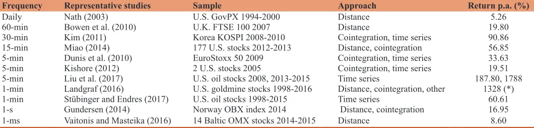
Table 1 provides a large range of back-testing high-frequency pairs trading strategies on different markets as well as at various

time frames. The relevant literature is ordered by increasing frequency. Research in pairs trading applied to high-frequency data is conducted in the most recent years while lower frequencies are examined in earlier years.

The first and most cited research study linked to high-frequency pairs trading is provided by Nath (2003). However, the author does not operate in a true high-frequency setting since tick data

of U.S. Treasury securities are aggregated to a daily average.

Nath (2003) diverges from the classic approach of Gatev et al. (1999; 2006) in terms of pairs selection and definition of trading signals. All securities for which there are at least ten quotes a day

are considered for constructing pairs and the trading signals are determined by the quantile of the normalized price series. In this

first high-frequency setting, returns of 5.26% p.a. are computed.

Bowen et al. (2010) further evaluate the high-frequency setting for the impact of transaction costs as well as other market frictions on the British stock market for the period January to December 2007. They identify a high sensitivity of returns to transaction

costs which reduce the trading results by a substantial amount.

By analyzing characteristics of returns over time they find that the

vast majority of trades is made in the 1st_{h of each day. The excess}

returns partly load on both market factor and reversal risk factor.

Kim (2011) presents the first study considering the Asian stock market for high-frequency pairs trading. Simultaneously, the author runs the cointegration and time series approaches to back-test the data. Kim (2011) suggests the strategy to be profitable

after transaction costs with a higher profitability in more volatile markets.

These findings are confirmed by Miao (2014) on a larger and more

liquid sample of 177 U.S. oil and gas companies. Using the S&P

500 as a benchmark, a strong performance is observed when the index produces opposite results. The author finds high returns of up to 56.85% p.a., also applying a cointegration algorithm for

pairs selection.

Dunis et al. (2010) employ their long-short strategy to stocks of the EuroStoxx50 index sampled at frequencies of 5, 10, 20, 30, 60 min and compare its profit potential to the results of trading based

on daily closing prices. Considering information ratio, for instance, the relation of annualized return to annualized standard deviation,

they find that intraday sampling intervals clearly outperform daily data - not surprising since mispricings on the market are corrected

at a faster pace.

Kishore (2012) only focuses on two stocks, Exxon Mobil

Corporation and Chevron Corporation, and provides a detailed analysis. Besides different allocation ratios to invest in pairs the author suggests an optimal width and level of the trading signal

threshold. Furthermore, the author finds dynamic trading bands as trading signals to generate more profitable results than the classic static trading bands computed in a preceding formation period. The

upper (lower) dynamic band is obtained by adding (subtracting) the multiple of the running standard deviation to (from) the running mean. Based on a long-term relationship of the stocks, Kishore (2012) cannot exploit cointegration for pairs selection.

Liu et al. (2017) use an Ornstein-Uhlenbeck process for modeling the price spread between two stocks. Specifically, they introduce

a doubly mean-reverting process using conditional modeling in order to secure mean-reversion of the spread. Thereby, the authors focus on a small long-term, however large intraday variance in

Table 1: Literature applying the pairs trading strategy to high-frequency data listed by increasing frequency. (*) An annual geometric mean is calculated since only daily returns of 104 basis points are available

Frequency Representative studies Sample Approach Return p.a. (%)

Daily Nath (2003) U.S. GovPX 1994-2000 Distance 5.26

60-min Bowen et al. (2010) U.K. FTSE 100 2007 Distance 19.80

30-min Kim (2011) Korea KOSPI 2008-2010 Cointegration, time series 90.86

15-min Miao (2014) 177 U.S. stocks 2012-2013 Distance, cointegration 56.85

5-min Dunis et al. (2010) EuroStoxx 50 2009 Cointegration, time series 33.63

5-min Kishore (2012) 2 U.S. stocks 2005 Cointegration, time series 19.51

5-min Liu et al. (2017) U.S. oil stocks 2008, 2013-2015 Time series 187.80, 1788

1-min Landgraf (2016) U.S. goldmine stocks 1998-2016 Distance, cointegration, other 1328 (*)

1-min Stübinger and Endres (2017) U.S. oil stocks 1998-2015 Time series 60.61

1-s Gundersen (2014) Norway OBX index 2014 Distance, cointegration 16.95

(3)

order to generate a large number of profitable trades. For empirical

study, the authors opt for oil stocks of NYSE and NASDAQ from both June 2013 to April 2015 and in 2008.

Recently, Stübinger and Endres (2017) develop a pairs trading framework applying a mean- reverting jump diffusion model to minute-by-minute data of the S&P 500 oil companies from 1998 to 2015. Using a 3-step calibration procedure to the spreads, they

are in position to perform intraday and overnight trading. In the

back-testing study, their strategy generates annualized returns of 60.61% and an annualized Sharpe ratio of 5.30 after transaction

costs.

Overall, pairs trading proves profitable when enhanced in different ways. Still, there always is the requirement to further improve the

strategy in order to escape the quick correction of mispricings on the market.

3. DATA AND SOFTWARE

The empirical study is performed on minute-by-minute stock prices of the S&P 500 index constituents from 1998 to 2015. This highly liquid subset contains the 500 largest companies of the U.S. stock market and covers approximately 80% of available market capitalization (S&P 500 Dow Jones Indices, 2015). The

data set serves as a representative basis to test any potential capital

market anomaly, given thorough investor scrutiny as well as global analyst reporting. We follow Krauss and Stübinger (2017)

and eliminate the survivor bias from our data using a two- stage

procedure. First, we use QuantQuote (2016) and create a daily constituent list that indicates which stock has been part of the index from January 1998 to December 2015. This information

is transferred into a binary matrix - columns represent all listed

stocks and rows describe the days from January 1998 to December 2015. If a company is a constituent of the S&P 500 index at the

current day, it is assigned a “1” at the corresponding element of the

matrix, otherwise a “0”. Second, the complete historical tick data for all stocks is downloaded from QuantQuote (2016), providing one quote for each time point a trade takes place. The prices are adjusted for stock splits, dividends, and further corporate actions.

In line with Stübinger and Endres (2017), the ticks are aggregated to minute-by-minute values, assigning a stock price to each minute. If the stock has not been traded from one minute to another, the

price from the previous time point is assigned to the current

one. By connecting both data sets, we obtain the S&P 500 index

constituency and the corresponding prices for each day.

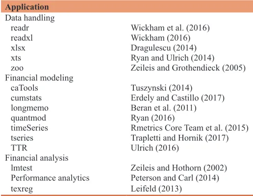
The financial modeling and results computing is conducted in the statistic programming language R. All additional software packages used are listed in Table 2.

4. CONSTRUCTING DIFFERENT PAIRS

TRADING STRATEGIES

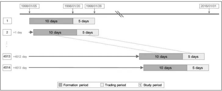
For our empirical application, we opt for minute-by-minute stock prices of the S&P 500 index constituents from January 1998 until December 2015 (see section 3). Following Jegadeesh and Titman

(1993) and Gatev et al. (1999; 2006), we split our data set into 4514 overlapping study periods, each shifted by 1 day (Figure 1). In the spirit of Bowen et al. (2010) and Kim (2011), each study period consists of a 10-day formation period (subsection 4.1) and an out-of-sample 5-day trading period (subsection 4.2). While the

former aims at identifying the most suitable pairs based on the

co-movement of the stocks, the latter relates to trade the top pairs applying predefined rules. Stocks that have become constituents or have been taken off during the formation period are not regarded in the study period. If stocks of top pairs leave the index during the

trading period, these pairs are removed and the returns achieved until this time point are recorded. Consequently, our portfolio strategy does not employ information that are from future - any

look-ahead bias is avoided.

Each day on the stock market begins at 9:30 am and ends at 4:00 pm, providing 391 mi-by-min data points for each stock per day. Typically, there are 500 stocks constituents of the

index for each 15-day study period. Hence, approximately

4514 15 500 391 = 1.32 * 1010_{stock prices are managed during}

one simulation run.

4.1. Selecting the Most Suitable Pairs

In the 10-day formation period, we follow Gatev et al. (1999; 2006) and focus on the portfolio of the 20 most suitable pairs

in terms of highest co-movement of the corresponding stocks. Typically, we select the top 20 pairs out of 500 499/2 = 124, 750 combinations of potential pairs. We aim at identifying pairs of two synchronous stocks, i.e., prices have historically moved

together. Therefore, the return time series of normalized prices for

each stock is calculated. Given that there does not exist a unique

measure for the co-movement of time series, we analyze three different approaches. The classic distance approach by Gatev et al.

(1999; 2006) monitors the Euclidean distance (E), i.e., the

straight-line distance between two points. The second selection process

computes the Pearson correlation coefficient (C) - a measure of

linear correlation between two variables. The approach based on

the fluctuation behavior (F) considers both standard deviation and Table 2: R packages used in this paper for data handling, financial modeling, and financial analysis

Application

Data handling

readr Wickham et al. (2016)

readxl Wickham (2016)

xlsx Dragulescu (2014)

xts Ryan and Ulrich (2014)

zoo Zeileis and Grothendieck (2005)

Financial modeling

caTools Tuszynski (2014)

cumstats Erdely and Castillo (2017)

longmemo Beran et al. (2011)

quantmod Ryan (2016)

timeSeries Rmetrics Core Team et al. (2015)

tseries Trapletti and Hornik (2017)

TTR Ulrich (2016)

Financial analysis

lmtest Zeileis and Hothorn (2002)

Performance analytics Peterson and Carl (2014)

(4)

mean-reversion speed of the spread. In the following subsections, we provide a detailed description of the three measures.

4.1.1. Euclidean distance (E)

In order to select historically co-moving pairs, Gatev et al. (1999; 2006) monitor the Euclidean distance of each possible stock pair

in the formation period. Those pairs with the smallest distance, therefore showing the closest co-movement, are allowed to enter

the trading period. In line with Gatev et al. (1999; 2006), this paper combines every constituent of the S&P 500 with another in a(typically) 500 × 500 matrix, the rows and columns each labeled according to the stocks of the index in the formation period. The

distance for each pair is calculated and recorded in the respective array of the matrix. Then, the strictly upper triangle matrix is retained since the lower triangle matrix shows the same pairs in a reversed order and the diagonal contains pairs of identical

stocks. Finally, the 20 pairs indicating the smallest distance enter

the subsequent trading period.

4.1.2. Correlation coefficient (C)

Chen et al. (2012) suggest to monitor the co-movement of stock

pairs by computing the Pearson correlation coefficient. The

coefficient is 1 in case of perfect increasing linear relationship, -1 in case of perfect decreasing linear relationship and 0 in case of no

linear relationship. High values indicate the most suitable pairs to trade in the future. The procedure resembles the Euclidean distance

approach. Similarly, in a 500 × 500 matrix, every correlation is

registered. In order to avoid duplication, only the strictly upper triangle is retained. Searching for highly correlated pairs, they are

now ordered by decreasing correlation coefficient. The 20 pairs

with the highest correlation are chosen to proceed to the trading period.

4.1.3. Fluctuation behavior (F)

The ideal pair to trade with this approach records a large number

of highly profitable trades. Therefore, Liu et al. (2017) create

a model in the time series approach where pairs are selected based on a small long-term, however large intraday variance.

In line with Liu et al. (2017), we transform this idea to the

distance approach. Pairs that are volatile and, at the same time,

quickly mean-reverting are identified in the formation period.

The volatility is measured by the standard deviation of the

spread, mean-reversion speed is calculated by the number of zero

crossings, which is defined as the number of times the spread crosses the mean (Do and Faff, 2010). Combined with the trading period approaches, this mean is either static (subsection 4.2.1) or time-varying (subsection 4.2.2 and 4.2.3). Pairs are ranked

separately for standard deviation as well as zero crossings where the pair holding the highest value for each measure is assigned

the highest rank. Consequently, the sum of the two separate ranks builds a combined rank. We achieve the top 20 pairs by choosing pairs with the highest composite rank.

4.2. Determining the Trading Rules

In the 5-day trading period, the selected pairs are traded according

to previously defined rules. For each top pair, we determine

individual trading thresholds based on the intention that we open

a long-short position, i.e., we buy the undervalued stock and short sell the overvalued stock when the respective spread diverges by a certain amount (Fernholz and Maguire, 2007). This entry threshold

is represented by the upper and the lower band which are obtained

by adding (subtracting) k-times the standard deviation to (from) the historical equilibrium (k ∈ℝ+_{). The position is closed when}

the spread reverts back to its historical equilibrium. If there is

an open trade at the end of the 5-day trading period, it is closed

automatically with either a profit or a loss being made. Naturally, there exist different definitions of the upper (lower) band and the historical equilibrium. In order to define the trading bands, our

study discusses three approaches. The approach static trading

thresholds (S) determines the trading signals by calculating the

mean and standard deviation of the spread during the formation

period. In contrast, the approaches time-varying thresholds (V) and reverting thresholds (R) use the running mean and the running

standard deviation, i.e., for every pair and every newly arriving

price per minute in the trading period, we update both key figures

always using the past 390 minutes. We note that our strategies

only use data available up to the respective time - this procedure

avoids any look-ahead bias. The approach time-varying thresholds (V) opens a trade when the spread crosses the upper (lower) band for the first time. Consequently, this method is the time-dynamic version of the approach employing static trading thresholds (S). On the other hand, the approach reverting thresholds (R) opens a trade when the spread crosses the upper (lower) band for the

second time.

(5)

4.2.1. Static thresholds (S)

Gatev et al. (1999; 2006) calculate the trading bands based on

the information of the formation period using the spread of the

respective stock pair. The mean of the spread over the entire 10-day

period indicates the historical equilibrium. The upper and lower

entry bands depict a divergence of k standard deviations from this mean - Gatev et al. (1999; 2006) use k = 2. Those straight bands are transferred to the trading period where the spread is tracked minute-by-minute. As soon as it crosses the upper or lower band,

a trade is opened. It is reversed, when the spread hits the historical mean, in the following. It should be mentioned that trading bands remain at the same value over the 5-day trading period regardless of trends followed by the spread.

4.2.2. Varying thresholds (V)

Kishore (2012) finds a better performance for dynamic trading

bands studying a 5-minute interval, since small deviations can have a substantial effect. Our study uses the Bollinger bands by

Bollinger (1992; 2001) which are applied by Stu¨binger et al. (2016) to calculate dynamic trading bands. The thresholds are

now computed and updated during the trading period at every time point instead of calculating three unique trading bands after

the formation period. A moving average for the mean and standard

deviation is calculated which adjusts to trends of the spread and is able to identify a divergence from this trend. For our 5-day trading period, we calculate the moving average and standard deviation for

the past 391 minutes, thus one trading day - a reasonable value since Jondeau et al. (2015) and Stu¨binger and Endres (2017) find that

overnight variations represent a substantial part in the context of

high-frequency data. For the first 390 minutes of a trading period,

we process the additional needed data from the formation period.

4.2.3. Reverting thresholds (R)

This set of trading bands is, similarly to the varying thresholds

(V), based on the dynamic trading bands by Bollinger (1992; 2001). We calculate a moving average and standard deviation for the past 391 minutes in the trading period. However, the time the trade is executed differs. Velayutham et al. (2010) suggest to

open a trade when the spread crosses an entry band for the second

time. Thereby, they look to secure mean-reversion of the spread.

If a spread drifts away from its mean but does not return, a trade should not be opened. In fact, if it is opened, large losses could be

generated. This risk should be avoided by waiting for the spread to change its direction and return to its mean. As a result, we open the trade according to Velayutham et al. (2010) upon crossing a

dynamic entry band for the second time. It is closed when hitting

the dynamic mean. Again, we use the data needed for the first 390 minutes of a trading period from the formation period.

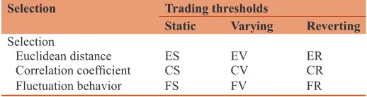
4.3. Generating Different Strategies

The selection process of the top pairs and the subsequent trading period can be regarded independently. That is why the different

approaches from the formation period (subsection 4.1) and trading period (subsection 4.2) can be combined without any restrictions. Considering three approaches each, that results in a 3 × 3 matrix

which includes nine different pairs trading strategies. Those are listed in Table 3. The approach is labeled by its first letter, e.g.,

E represents Euclidean distance for pairs selection, S describes

static trading thresholds, etc.. Each strategy is described by two

letters, the first showing the selection process and the second

the trading rules applied. Consequently, the strategy ES selects pairs based on the Euclidean distance and possess static trading thresholds.

4.4. Return Computation

Return calculations is based on Gatev et al. (1999; 2006). Specifically, the sum of daily payoffs across the portfolio is

scaled by the sum of invested capital at the previous day’s end. We report both the return on employed capital, i.e., investing one USD for each active pair, and the return on committed capital, i.e., investing one USD for each pair. In most cases, we depict return on employed capital which is the more common metric in the literature and practice.

4.5. Market Frictions

In this subsection, we discuss our high-frequency strategy in light

of market frictions. Most notably, we discuss the financial costs

and the technical effort of implementing the presented strategies as

well as the lack of any survivor bias in our back-testing framework. However, we find that the designed pairs trading framework satisfy

practical constraints.

First, for every activity conducted on the market, there is a transaction cost linked to it. Since a high-frequency pairs trading strategy is based on permanent trading on the market, it would be naive to ignore those charges. While Do and Faff (2012)

state that the exact magnitude of transaction costs cannot be determined, data shows a considerable decrease in the recent

past of 2012. Following Avellaneda and Lee (2010) and Krauss (2017), this paper applies transaction costs of 5 basis points per

share per half-turn. This assumption is well in conformity with

diverse studies in pairs trading research. While Bogomolov (2013) accentuates that even retail commissions account for 10 basis points per transaction, Do and Faff (2012) assume institutional commissions of 10 basis points or less from 1997 to 2009. Brogaard et al. (2014) point out that high-frequency trading is a

liquidity providing strategy exploiting transitory pricing errors and, thus, potentially convenient for rebates. Consequently, any

further market impact is not taken into account. However, market impact would be close to zero for the S&P 500. Estimating exact values is exceedingly difficult but Prager et al. (2012) show that the bid-ask spread has abated to <1% for the stock of the S&P 500 index, i.e., 2 basis points for an average stock price of 50 USD. Krauss and Herrmann (2017) confirm this estimation reporting bid-ask spreads of 4-5 basis points on a high-frequency data set of the DAX 30 constituents. Voya Investment Management (2016) report a bid-ask spread of 3.5 basis points for the S&P 500

Table 3: Crosswise combining the different approaches in a 3×3 matrix to generate nine pairs trading strategies

Selection Trading thresholds

Static Varying Reverting

Selection

Euclidean distance ES EV ER

Correlation coefficient CS CV CR

(6)

caused by changes in the exchange landscape, decimalization, and increased use of algorithmic trading. Our strategy is quite aggressive, however, it proves feasible given our high-turnover strategy of an institutional trader on minute-by-minute prices. We

are operating in a highly liquid stock market universe which covers approximately 80% of available market capitalization, implying

no further capacity constraints.

Second, the computational run time of our implemented trading strategies does not arise problems caused by practical feasibility. In reality, selecting the most suitable pairs is conducted over night,

which is why the run time must not exceed 63,000 s (time period between 4:00 pm and 9:30 am). Due to the minute-by-minute

frequency of the incoming data, determining the dynamic trading

rules must be computed in <1 min. Parallelized processing on 8 hyper threads on a contemporary Intel core i7-6700 HQ with a clock speed of 2.6 GHz leads to an approximate average run time of 4.63 s for the formation period and 1.02 seconds for the

complete trading period per study period, i.e., newly arriving prices

are handled in approximately 0.0005 seconds. Consequently, we

are in position to trade without any time restrictions. Clearly,

these key figures are determined based on the computing power

of a modern computer. Moore (1965; 1975) finds that the number

of transistors on integrated circuits doubles approximately every

24 months. Accordingly, the increase of the computing power is 512-fold (= 29_{) over our study period from 1998 to 2015.} Effectively, the run time during the first years of our study period amounts to 4.63 512 = 2371 seconds for the formation period and to 0.0005 512 = 0.256 seconds for the trading period - both values

cause no technological constraints for our strategy. Consequently,

the trading framework could have been implemented given the

technology in the early part of the sample without any technical restrictions.

Third, we only use information which was available at the time those strategies were designed. While the concept of the Euclidean distance is based on the Pythagorean theorem, the correlation

coefficient is developed by Pearson (1895). The approach fluctuation behavior employs the standard deviation and the mean-reverting speed of the spread - both well known for a long

time. The same applies to the approach based on static trading thresholds which handles the mean and the standard deviation. The approaches applying varying thresholds and reverting thresholds

use the Bollinger bands which are first introduced by Bollinger (1992). Concluding, our strategies only convert information which

has been realized and, simultaneously, use data available up to the respective time during the trading period - this procedure avoids

any look-ahead bias.

5. RESULTS

5.1. Choosing the Parameter Setting of the Strategies Table 4 reports mean returns per year as well as annualized

Sharpe ratios for the top 20 pairs of the presented strategies after

transaction costs. Therefore, we vary the way of selecting the most suitable pairs in terms of co-movement (subsection 4.1), the method of determining the trading rules (subsection 4.2), and the trading thresholds based on k standard deviations. Following

Gatev et al. (1999; 2006) as well as Bollinger (1992; 2001), we set k = 2 as starting point and vary the parameter k in two directions (k ∈ {1, 1.5, 2, 2.5, 3}).

Regarding the selection of the most suitable pairs, we observe

that the strategies applying the correlation coefficient (C)

produce clearly lower results than those employing euclidean

distance (E) and the fluctuation behavior (F). This fact is not

surprising since high correlation and a cointegration relationship

are not affiliated directly with each other. Consequently, there

does not exist a theoretical foundation that divergences are

followed by any mean-reversions (Alexander, 2001). Spurious

relationships lead to higher probability of momentum pairs and,

thus, to financial losses - an undesired property for any rational

investor. Nonetheless, it has to be pointed out that the annualized returns, including one exception, are always positive with a

maximum of 37.85% p.a. Annualized returns after transaction

costs are similar for strategies performing the approaches E and F. Considering the Sharpe ratio, i.e., the excess return per unit of deviation, we see that approach E is particularly suitable for selecting the top pairs - the global maximum of the Sharpe ratio with a value of 8.14 is also achieved by this method. This is due to the fact that approach F selects pairs with both a high spread variation and strong mean-reversion properties resulting in frequent and substantial divergences from the equilibrium. Consequently, the returns of the respective trades possess a high variance implicating a relatively low Sharpe ratio. The vast majority of literature on daily data animadvert on selecting pairs with E because an ideal pair exhibits a spread of zero and, thus,

generates no profits. Since strategies using this approach possess

the best results in our application, we may carefully conclude that

this drawback is eliminated by the naturally higher variations of

the high-frequency data.

Table 4: Yearly returns and Sharpe ratios for the top 20 pairs for the nine pairs trading strategies after transaction costs from January 1998 until December 2015

Strategy Return Sharpe ratio

S V R S V R

k=1

E 0.3036 0.2389 −0.6629 4.6672 1.8818 −15.4011

C 0.0425 0.1196 −0.5482 0.3504 0.8183 −7.5086

F 0.0651 2.5190 −0.5541 0.2154 5.9196 −2.9137 k=1.5

E 0.2933 0.5213 −0.3945 5.1433 5.4074 −9.4403

C 0.0282 0.3111 −0.3527 0.1261 2.7059 −4.8238 F 0.0907 0.9345 −0.4375 0.3162 3.4146 −2.3254

k=2

E 0.2552 0.5726 −0.1960 4.9565 7.5135 −5.3947

C 0.0406 0.3785 −0.2129 0.3286 3.8191 −3.2292

F 0.1804 0.5375 −0.3596 0.6467 2.2121 −2.0071 k=2.5

E 0.2152 0.5050 −0.0898 4.4379 8.1404 −3.1485 C 0.0689 0.3646 −0.1281 0.7810 4.1965 −2.2920

F 0.3706 0.3751 −0.2794 1.2042 1.6842 −1.6735

k=3

E 0.1843 0.4225 −0.0273 3.8801 8.0478 −1.6239

C 0.0576 0.3193 −0.0778 0.7020 4.0091 −1.7938

(7)

Considering the determination of the trading rules, we observe an unambiguous result about the performance of the different

approaches: Strategies composed of varying thresholds (V) clearly outperform static thresholds (S) and reverting thresholds (R) - the last approach reveals as the weakest method. The large deviation

of V and R is a clear evidence that crossing the Bollinger bands

for the first time indicates a temporal market inefficiency, while

passing these for the second time depicts no particular change in prices. Naturally, strategies based on R are not protected from pairs where closing is forced at the end of the 5-day trading period. That is why all strategies with this approach result in

negative annualized returns and Sharpe ratios. Applying approach

S does not imply a large number of trades which is, however,

essential for any trading strategy (details about trading statics can be found in the next subsection). Nevertheless, this method produces substantial annualized returns ranging from 2.82% to 50.63% from 1998 until 2015 after transaction costs. On the

opposite, strategies using V exhibit the highest returns in almost all cases - through many trades being executed. Consequently,

our assumptions hold and the Bollinger bands efficiently provide a relative definition of high and low. Overall, the findings of Kishore (2012) are confirmed that the results of varying trading thresholds are superior in terms of risk and return characteristics due to their high flexibility.

In contrast to the pairs trading literature on daily data, bilateral

comparisons lead to the finding that pairs trading strategies using k = 2.5 standard deviations achieve the highest level of

performance. This circumstance is not unexpected since

high-frequency prices exhibit more fluctuation resulting in higher

transaction costs. We may carefully conclude that the use of

k = 2.5 provides the most favorable combination of meaningful

divergences as well as a certain quorum of trades in the context of minute-by-minute data.

In the following subsections, we focus on the nine different

strategies based on k = 2.5, given that this parameter produces the most successful risk-return results. In line with Yu (2006),

we evaluate the risk-return characteristics and trading statistics, conduct a sub-period analysis, and check the exposure to common systematic risk factors. The vast majority of the applied performance metrics is considered by Bacon (2008).

5.2. Outperformance of Euclidean Distance and Varying Thresholds

Table 5 depicts daily return characteristics and risk metrics for the top 20 pairs per strategy from January 1998 to December 2015 compared to a simple buy-and-hold strategy of the S&P 500 as a benchmark (MKT). We observe statistically significant returns for strategies using static thresholds (S) and varying thresholds (V),

with Newey-West t-statistics above 3.13 after transaction costs.

From an economic perspective the returns are significant as well, ranging between 0.03% per day for strategy CS and 0.16% per day for strategy EV. As expected, strategies based on reverting thresholds (R) combined with all three selection processes produce negative returns ranging from −0.12% to −0.04% per day - decisively inferior to the 0.02% of the general market. In contrast to strategies employing Euclidean distance (E) or correlation coefficient (C), the approach fluctuation behavior (F)

produces results with strong outliers - compare both the minimum and maximum. This picture barely changes considering the

variation of the returns. Again, strategies applying E and C

generate returns with low standard deviations while F presents

returns with standard deviations up to 1.79%, compared to 1.26% for the S&P 500 benchmark. These findings are not astonishing

since selecting pairs with F aims at identifying pairs with a large

volatility of their spread. All strategy variants selecting pairs with E or C show right skewness and follow a leptokurtic distribution

- a favorable characteristic for any potential investor and out of

character for financial data (Cont, 2001). We follow the approach of Mina and Xiao (2001) and analyze the Value at Risk (VaR) measures of the different strategies. Tail risk for strategies using

E and C is greatly reduced compared to an investment in the S&P

500 (VaR 1% at −3.50%) and strategies performing V (VaR 1% ranges between −4.60% and −4.09%). Especially, strategy EV outperforms with a VaR 1% of −0.32% and a VaR 5 % of −0.43%.

Table 5: Daily return characteristics for the top 20 pairs of the nine pairs trading strategies after transaction costs compared to a S&P 500 long-only benchmark (MKT) from January 1998 until December 2015. NW denotes Newey–West standard errors with 5-lag correction and CVaR the conditional value at risk

Feature ES EV ER CS CV CR FS FV FR MKT

Mean return 0.0008 0.0016 −0.0004 0.0003 0.0012 −0.0005 0.0014 0.0014 −0.0012 0.0002

Standard error (NW) 0.0001 0.0001 0.0001 0.0001 0.0001 0.0001 0.0003 0.0002 0.0002 0.0002 t-statistic (NW) 11.4728 13.7734 −5.4549 3.1374 10.9571 −6.3491 4.7000 5.8194 −6.2594 1.0010

Minimum −0.0148 −0.0082 −0.0081 −0.0336 −0.0398 −0.0364 −0.3718 −0.1473 −0.1607 −0.0947

Quartile 1 −0.0005 −0.0006 −0.0017 −0.0013 −0.0011 −0.0022 −0.0028 −0.0025 −0.0039 −0.0056

Median 0.0003 0.0005 −0.0009 0.0001 0.0007 −0.0008 0.0004 0.0015 −0.0003 0.0006

Quartile 3 0.0014 0.0029 0.0004 0.0017 0.0029 0.0008 0.0056 0.0062 0.0030 0.0061

Maximum 0.0673 0.0434 0.0202 0.0666 0.0658 0.0645 0.2359 0.0812 0.0874 0.1096

Standard deviation 0.0027 0.0037 0.0022 0.0038 0.0051 0.0040 0.0179 0.0130 0.0111 0.0126

Skewness 6.9416 2.8295 1.7202 1.9267 1.7948 1.3628 −2.1390 −1.8527 −3.1598 −0.2003 Kurtosis 118.2404 17.5882 6.2217 33.5926 21.4766 28.2527 70.6366 19.9597 33.4605 7.5475

Historical VaR 1% −0.0031 −0.0032 −0.0038 −0.0084 −0.0105 −0.0109 −0.0460 −0.0422 −0.0409 −0.0350 Historical CVaR 1% −0.0045 −0.0043 −0.0049 −0.0133 −0.0169 −0.0166 −0.0858 −0.0691 −0.0662 −0.0503 Historical VaR 5% −0.0018 −0.0019 −0.0029 −0.0047 −0.0047 −0.0053 −0.0194 −0.0158 −0.0161 −0.0196 Historical CVaR 5% −0.0027 −0.0028 −0.0036 −0.0076 −0.0086 −0.0091 −0.0399 −0.0335 −0.0325 −0.0302

Maximum drawdown 0.1080 0.3983 0.9800 0.2944 0.3188 0.9518 0.4637 0.3331 0.9973 0.6433

(8)

Most interestingly, the maximum drawdown, i.e., the decline from

a historical peak, is at a very high level for strategies employing

reverting thresholds. The hit rate, i.e., days with positive returns,

underlines our results. Strategy EV exhibits up to 61.07% which

proves superior to all other trading strategies. Concluding, strategy

EV generates favorable return characteristics and risk metrics - this finding confirms the statements of Kishore (2012).

In the spirit of Emna and Chokri (2014), Table 6 presents the trading statistics of all nine strategies. Including two exceptions,

out of 20 pairs almost all of them are traded. Applying strategies CS and FS, however, only 12.92 and 6.93 pairs are traded during the 5-day trading period. That is in line with Do and Faff (2010) who find that the simple pairs trading approach with static trading thresholds by Gatev et al. (1999; 2006) performs weaker for high-frequency data. Working with high-frequency prices, small

deviations of the spread can have a large impact since static trading bands cannot adjust to the change - drifts and volatility cluster are completely neglected. Consequently, trading will not

be possible anymore. This is confirmed by the number of

round-trips. While strategies employing V and R, which are both based on dynamic thresholds, generate 4 to 6 round-trips per pair, this number is only between 1 and 2 for strategies performing S.

Applying time-varying thresholds, pairs close quickly within one day. That is desired by investors since they may quickly reinvest their capital and do not bear the risk of losing money on

an open position. For static trading thresholds, pairs are open for

2-3 days which does not allow for a large number of profitable trades. Furthermore, most of those pairs have to be forced to close at the end of the trading period since they do not revert to their static mean. That is most visible for the E approaches, where on average 15 pairs have to be closed by force for S compared to 6-7 for V and R.

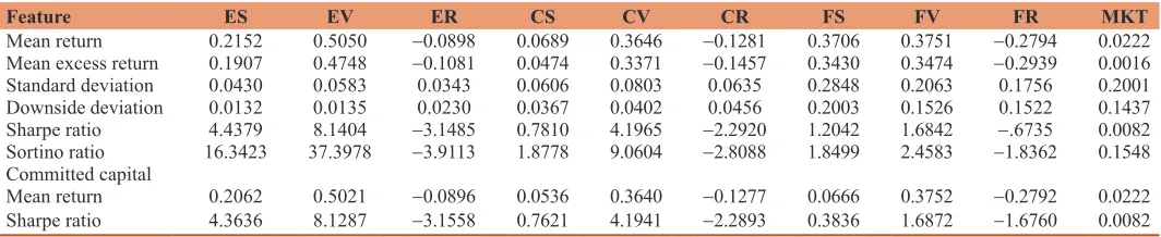
The annualized risk-return measures for the pairs trading

strategies are shown in Table 7. Since we base our statistics on employed capital, the returns applying committed capital are

listed at the bottom. We reach up to 50.50% annualized return

when selecting by minimum Euclidean distance and trading

with time-varying trading thresholds (Strategy EV), followed by 37.51% by the FV strategy. Mean return calculations using

committed capital identify only slightly smaller, since almost all pairs are traded during the 5-day trading period. Large differences between employed and committed capital mean return calculation

are observed for the strategies CS and FS (Table 6). Findings by Dunis et al. (2010) and Kishore (2012) are confirmed that high-frequency pairs trading proves to be less volatile than the market. Compared to the S&P 500, only volatile pairs selected by F show a similar standard deviation. All other strategies are less volatile.

Strategies based on V yield, for every pairs selection approach, the best Sharpe ratios, e.g., strategy EV achieves a favorable Sharpe ratio of 8.14 after transaction costs. Summarizing, the strategy

selecting pairs on Euclidean distance (E) and using varying thresholds (V) displays the most attractive return characteristics and trading statistics: Statistically and economically significant

returns, a greater number of pairs traded per 5-day period and a low time pairs remain open.

5.3. The Declining Profitability in Pairs Trading Over

Time

Do and Faff (2010), Bowen and Hutchinson (2016), and Stu¨binger and Endres (2017) report declining performance over time in their back-testing of pairs trading strategies. In the following, we analyze whether the presented strategies are influenced by time

effects. Table 8 presents annualized risk-return measures for every trading approach (static thresholds (S), varying thresholds (V), reverting thresholds (R)) combined with each of the selection processes (Euclidean distance (E), correlation coefficient (C), fluctuation behavior (F)). The time frame analyzed from January 1998 to December 2015 is split up into six sub-periods. Since we use the S&P 500 as a benchmark, an index containing U.S. stocks only, we need to analyze the strategies regarding the U.S. market and the events influencing it.

In the years leading to 2000, the U.S. economy is growing under

president Bill Clinton. Simultaneously, there is no wide range of high-frequency trading, since progress in technology is yet to come in the following years. Thus, all strategies made use of a

rather slow correction of mispricings on the market. Annualized returns range between −38.80% for strategy FR and 302.96% for

EV. This period is characterized by low standard deviations and,

thus, high Sharpe ratios which makes it a highly attractive trading

strategy at that time.

Stübinger and Endres (2017) identify a turbulent period from 2001 to 2003 which comprises the dot-com crash, the 9/11 attacks, and the subsequent Iraq war. Although the market shows negative returns of −7.81% p.a., pairs trading still performs extremely well.

Table 6: Trading statistics for the top 20 pairs of the nine pairs trading strategies per 5-day trading period from January 1998 until December 2015

Feature ES EV ER CS CV CR FS FV FR

Average number of pairs traded per 5-day

period 19.0366 19.9276 19.9271 12.9158 19.9623 19.9623 6.9291 19.9920 19.9920

Average number of round-trip trades per pair 1.9665 6.0067 5.9614 1.2727 5.2068 5.1768 1.0140 4.7930 4.7745 Standard deviation of number of round-trip

trades per pair 2.5977 2.6865 2.6281 2.7061 1.8511 1.8130 0.1248 1.3321 1.3255

Average time pairs are open in days 1.6203 0.3956 0.3820 2.5660 0.5346 0.5069 3.4070 0.6319 0.5921

Standard deviation of time open, per pair,

in days 1.5416 0.4114 0.4025 1.7486 0.4607 0.4408 1.5339 0.4871 0.4621

Average number of pairs where closing is

(9)

Table 7: Annualized risk-return measures for the top 20 pairs of the nine pairs trading strategies after transaction costs compared to a S&P 500 long-only benchmark (MKT) from January 1998 until December 2015

Feature ES EV ER CS CV CR FS FV FR MKT

Mean return 0.2152 0.5050 −0.0898 0.0689 0.3646 −0.1281 0.3706 0.3751 −0.2794 0.0222

Mean excess return 0.1907 0.4748 −0.1081 0.0474 0.3371 −0.1457 0.3430 0.3474 −0.2939 0.0016

Standard deviation 0.0430 0.0583 0.0343 0.0606 0.0803 0.0635 0.2848 0.2063 0.1756 0.2001

Downside deviation 0.0132 0.0135 0.0230 0.0367 0.0402 0.0456 0.2003 0.1526 0.1522 0.1437

Sharpe ratio 4.4379 8.1404 −3.1485 0.7810 4.1965 −2.2920 1.2042 1.6842 −.6735 0.0082

Sortino ratio 16.3423 37.3978 −3.9113 1.8778 9.0604 −2.8088 1.8499 2.4583 −1.8362 0.1548

Committed capital

Mean return 0.2062 0.5021 −0.0896 0.0536 0.3640 −0.1277 0.0666 0.3752 −0.2792 0.0222

Sharpe ratio 4.3636 8.1287 −3.1558 0.7621 4.1941 −2.2893 0.3836 1.6872 −1.6760 0.0082

The lowest annualized return generated by the strategies composed

of approach V is still as high as 77.39%. Standard deviations are

slightly higher compared to the previous sub-period, however, only

volatile strategies based on F exceed the benchmark.

A period of moderation follows from 2004 to 2006. The market denotes positive returns of 7.87% with a low volatility. Since pairs trading generates its profits from deviations of volatile stocks, conditions for successful trading are not provided. In fact, only strategies using time-varying thresholds (V), yield

consistently positive excess returns - Sortino ratios range between

1.91 for FV and 9.70 for CV, compared to 1.09 for the general market.

Into the period from 2007 to 2009 falls the global financial crisis as well as a deteriorating market. Returns decrease to an all-time

low while the standard deviations reach an all-time high of all six

observed sub-periods. In line with Kim (2011) and Miao (2014), we find that pairs trading performs exclusively well during that

time. Strategies applying S and V list high positive returns. In an

insecure market, the strategies employing approach F, especially, prove successful. With 70.03% for static and 117.84% for varying trading thresholds, a selection process using fluctuation behavior of prices works best during market downturns.

In 2010 to 2012, the U.S. market recovers while being affected by the European debt crisis to a small extent. Also, by this time almost all investors trade at a high-frequency market which results in a quick correction of mispricings on the market. Now, the simple pairs trading strategies introduced by Gatev et al. (1999; 2006)

become ineffective. Only the more complex strategies based on

F yield significant returns with a Sharpe ratio exceeding 2 for

strategy FV.

The final period from 2013 to 2015 confirms findings by various authors such as Do and Faff (2010) and Krauss et al. (2017). Returns and excess returns are identical since the risk-free rate at this time is 0. Profits of pairs trading decline over time. Market anomalies are instantly corrected and the market displays high returns with a low volatility as from 2004 to 2006. In order to set

up successful pairs trading strategies, more complex approaches

and potentially an even higher frequency are necessary. Stu¨binger and Endres (2017), for instance, develop a time series approach that does not follow the trend of a declining profitability using

a more advanced approach and additional information such as overnight trading. Nevertheless, the strategy FS depicts annualized

returns of 15.19% after transaction costs, although this strategy possesses a low number of pairs traded (Table 6). We may carefully conclude that only certain divergences are traded - A successful

strategy in recent times.

Figure 2 displays the cumulative return from 1998 to 2015 when making an initial investment of one USD. The best performing strategy applying static thresholds (S) selects pairs based on their fluctuation behavior (F). That is, as well, the only strategy

resisting the downward trend in recent years. Strategies composed

of varying thresholds (V) exhibit considerably higher cumulative returns, however, a decline in profits can be observed beginning in 2010. Finally, all strategies employing reverting thresholds present their weak performance by generating cumulative returns below the benchmark.

5.4. Partly Loading of the Best Performing Strategy on any Systematic Sources of Risk

Finally, we analyze the exposure of the strategy EV to common

systematic sources of risk. We employ three types of regression, following Knoll et al. (2017). First, the standard three-factor model (FF3) of Fama and French (1996) is used to capture the sensitivity to the overall market, small minus big capitalization stocks (SMB), as well as high minus low book-to-market stocks (HML). Second, we apply the Fama-French 3+2-factor model (FF3+2) as outlined in Gatev et al. (1999; 2006). It enhances the first model by a momentum factor and a short-term reversal factor. Third, we follow Fama and French (2015) and extend the baseline model by two additional factors, i.e., portfolios of stocks with a robust minus weak profitability (RMW) and with a conservative minus aggressive (CMA) investment behavior. This regression is called Fama-French 3+2 factor model (FF5). We download all data related to these models from Kenneth R. French’s website.1

Findings for the top 20 pairs of strategy EV after transaction costs

are summarized in Table 9.

Irrespective of the factor model employed, we see that the returns

depict statistically and economically significant daily alphas between 0.15 and 0.16% per day after transaction costs - similar to the raw returns. The exposure to the general market shows significant negative loading in case of the FF3+2 model - not surprising, given that our strategy is dollar neutral, not market

neutral. Therefore, FF3 and FF5 report no loading on this

1 We thank Kenneth R. French for providing all relevant data for these

(10)

Table 8: Annualized risk-return measures for the top 20 pairs of the pairs trading strategies based on static thresholds (S), varying thresholds (V) and reverting thresholds (R) after transaction costs compared to a S&P 500 long-only

benchmark (MKT) for sub-periods of 3 years from January 1998 until December 2015

I. Static thresholds (S) FS CS FS MKT ES CS FS MKT

Mean return 1998-2000 0.9120 0.1010 0.6031 0.0905 2001-2003 0.4157 0.1951 0.3826 −0.0781

Mean excess return 0.8189 0.0473 0.5250 0.0373 0.3856 0.1697 0.3532 −0.0978

Standard deviation 0.04960 0.0915 0.2387 0.2028 0.0460 0.0709 0.3634 0.2184

Downside deviation 0.0118 0.0634 0.1381 0.1417 0.0115 0.0375 0.2747 0.1538

Sharpe ratio 16.5237 0.5169 2.1992 0.1839 8.3835 2.3914 0.9718 −0.4478

Sortino ratio 76.9869 1.5934 4.3656 0.6390 36.0489 5.1996 1.3929 −0.5080

Mean return 2004-2006 0.0179 −0.0330 0.2483 0.0787 2007-2009 0.1312 0.1872 0.7003 −0.1177

Mean excess return −0.0116 −0.0609 0.2123 0.0475 0.1079 0.1628 0.6654 −0.1358

Sharpe ratio −0.5929 −1.4925 0.8196 0.4542 1.9024 2.5580 1.6041 −0.4534

Sortino ratio 1.4592 −1.0875 1.3538 1.0935 6.8782 7.2117 2.3312 −0.5328

Mean return 2010-2012 −0.0040 −0.0077 0.2255 0.0671 2013-2015 0.0442 −0.0044 0.1519 0.1182

Mean excess return −0.0048 −0.0084 0.2245 0.0663 0.0442 −0.0044 0.1519 0.1182

Sharpe ratio −0.1653 −0.2599 1.2077 0.3572 1.5734 −0.1040 0.9867 0.9222

Sortino ratio −0.3243 −0.3329 2.0166 0.5004 4.4783 −0.1873 1.5475 1.3058

II. Varying thresholds (V) EV CV FV MKT EV CV FV MKT

Mean return 1998-2000 3.0296 0.4247 0.2160 0.0905 2001-2003 1.4675 1.2272 0.7739 −0.0781

Sharpe ratio 48.8812 2.9951 0.7255 0.1839 22.1000 11.6011 2.7019 −0.4478

Sortino ratio 507.9948 5.6843 1.2900 0.6390 196.7001 31.1033 3.8980 −0.5080

Mean return 2004-2006 0.0448 0.2200 0.2816 0.0787 2007-2009 0.3211 0.8554 1.1784 −0.1177

Sharpe ratio 0.5984 4.4502 1.3944 0.4542 5.1434 9.8672 4.0613 −0.4534

Sortino ratio 3.1860 9.7040 1.9092 1.0935 20.7597 37.9979 6.1120 −0.5328

Mean return 2010-2012 −0.1021 −0.0680 0.2715 0.0671 2013-2015 −0.0426 −0.0336 −0.1177 0.1182

Mean excess return −0.1028 −0.0687 0.2706 0.0663 −0.0426 −0.0336 −0.1177 0.1182

Sharpe ratio −3.6359 −1.8464 2.1658 0.3572 −1.3303 −0.7444 −1.2807 0.9222

Sortino ratio −5.4533 −2.3760 2.9695 0.5004 −2.9159 −1.1954 −1.6536 1.3058

III. Reverting thresholds (R) ER CR FR MKT ER CR FR MKT

Mean return 1998-2000 0.6813 −0.1127 −0.3880 0.0905 2001-2003 0.1724 0.2710 −0.3923 −0.0781

Mean excess return 0.5994 −0.1560 −0.4179 0.0373 0.1474 0.2440 −0.4053 −0.0978

Sharpe ratio 15.5299 −1.5340 −2.4676 0.1839 4.3099 2.8383 −1.7197 −0.4478

Sortino ratio 55.6534 −1.4510 −2.5679 0.6390 11.4537 5.8917 −1.8573 −0.5080

Mean return 2004-2006 −0.2712 −0.2040 −0.3000 0.0787 2007-2009 −0.1881 −0.0372 −0.0783 −0.1177

Mean excess return −0.2923 −0.2270 −0.3202 0.0475 −0.2048 −0.0570 −0.0973 −0.1358

Sharpe ratio −18.5552 −6.9169 −2.1876 0.4542 −6.1638 −1.0662 −0.3860 −0.4534

Sortino ratio −10.7836 −6.3300 −2.2159 1.0935 −6.9572 −1.1359 −0.3860 −0.5328

Mean return −0.2977 −0.2949 −0.1724 0.0671 2013-2015 −0.2992 −0.2780 −0.2969 0.1182

Mean excess return 2010-2012 −0.2982 −0.2955 −0.1730 0.0663 −0.2992 −0.2780 −0.2969 0.1182

Sharpe ratio −17.3956 −9.6593 −1.7008 0.3572 −18.6153 −9.8720 −4.1134 0.9222

Sortino ratio −11.0093 −8.2796 −1.9747 0.5004 −11.4416 −8.7458 −4.4834 1.3058

factor. The SMB factor indicates a slightly significant loading - astonishingly, since we invest solely in large capitalization stocks. However, the results of Chan et al. (2002) and Krauss and

Stübinger (2017) exhibit similar anomalies relating to large cap mutual funds. Chen and Bassett (2014) explain this inconsistency

by proving that the Fama-French model can attribute small size to

(11)

short-term losers and shorts short-term winners. Also, we observe insignificant and very close to zero loadings for the factors HML, SMB5, HML5, RMW5, and CMA5. Highest explanatory power

is achieved by the FF3+2 model. Concluding, the strategy based

on Euclidean distance (E) and varying thresholds (V) produces significant returns, clearly outperforms the general market, and possesses almost no loading on systematic sources of risk.

6. CONCLUSION

In the first part of our article, we present a comprehensive literature

overview of pairs trading in the context of high-frequency data.

We find that using intraday stock prices in pairs trading research

started at 2010 - the closer we are to the present, the higher trading

frequencies are applied to the strategies. This circumstance is not unexpected since progress in research as well as increasing computing capacities allow to handle larger amounts of data within a shorter period of time.

The second part presents an extensive comparison study of nine different strategies in the formation and trading period. Therefore, we vary the process of selecting the most suitable pairs based on

the Euclidean distance (E), the correlation coefficient (C) and the fluctuation behavior (F). Different trading rules are regarded for trading the top pairs, i.e., we consider static thresholds (S), varying thresholds (V) and reverting thresholds (R). We construct Table 9: Exposure to systematic sources of risk for daily returns of the top 20 pairs for the strategy based on EV after transaction costs from January 1998 until December 2015. Standard errors are depicted in parentheses

Feature FF3 FF3+2 FF5

Intercept 0.0016*** (0.0001) 0.0015*** (0.0001) 0.0016*** (0.0001)

Market −0.0084 (0.0043) −0.0208*** (0.0047) −0.0079 (0.0050)

SMB −0.0174* (0.0086) −0.0153 (0.0086)

HML 0.0035 (0.0081) 0.0043 (0.0087)

Momentum −0.0095 (0.0060)

Reversal 0.0382*** (0.0061)

SMB5 −0.0136 (0.0093)

HML5 0.0100 (0.0092)

RMW5 0.0121 (0.0120)

CMA5 −0.0138 (0.0147)

R2 _0.0023

Adjust R2 _0.0012

Number observe 4518

RMSE 0.0036

***P<0.001, **P<0.01, *P<0.05. SMB: Small minus big, HML: High minus low, RMW: Robust minus weak, CMA: Conservative minus aggressive

Figure 2: Development of an investment of one USD for the top 20 pairs of the pairs trading strategies based on static thresholds (S), varying thresholds (V) and reverting thresholds (R) after transaction costs compared to a S&P 500 long-only benchmark (MKT) from January 1998 until

(12)

the classic pairs trading approach (Gatev et al., 1999; 2006)

by combining the Euclidean distance with static thresholds.

Furthermore, different market frictions are discussed, e.g., we consider the financial costs and technical effort of implementing the presented strategies as well as the lack of any survivor bias.

For our large-scale empirical study, we perform the different

strategies on minute-by-minute data of the S&P 500 constituents from January 1998 until December 2015. In our evaluation, we analyze the risk-return characteristics and trading statistics, perform a sub-period analysis, and check the exposure to common systematic risk factors.

Our findings possess a number of key takeaways and implications for theoreticians and practitioners. First, we find that the best performing results are achieved by determining the upper (lower) band by adding (subtracting) 2.5-times the standard deviation to (from) the mean. Using the parameter setting suggested by literature

on daily data reveals too aggressive, given that the higher trading frequency produces larger transaction costs which can obviously not

be compensated by increasing returns. Second, the most profitable pairs can be found by selecting pairs applying Euclidean distance and trading with varying thresholds. This constellation generates

statistically and economically significant returns of 50.50% p.a.

and an annualized Sharpe ratio of 8.14 after transaction costs. The

returns exhibit a strongly limited tail risk, e.g., the historical VaR 1 % is −0.32%, and indicate almost no loading on systematic sources of risk. Third, a sub-period analysis over all nine strategies reports strong pairs trading performance during times of severe market turmoil, i.e., the dot-com crisis or the global financial crisis. We confirm the statement of Gatev et al. (1999; 2006) and Do and Faff (2010) that pairs trading strategies show a declining trend over time. Notably, pairs trading based on fluctuation behavior and static thresholds presents an annualized return of 15.19% during 2013 until 2015 after transaction costs. Concluding, there still exist some pairs

trading strategies achieving pleasant performance in recent times.

For future research in this field, theoreticians and practitioners should adapt their trading strategy on the prevailing market conditions. Therefore, potential work should apply a

mixed-strategy with both pairs selection and trading thresholds depending

on the current market circumstances.

REFERENCES

Alexander, C. (2001), Market Models: A Guide to Financial Data Analysis. Chichester, UK and New York, NY: John Wiley and Sons.

Avellaneda, M., Lee, J.H. (2010), Statistical arbitrage in the US equities market. Quantitative Finance, 10(7), 761-782.

Bacon, C.R. (2008), Practical Portfolio Performance: Measurement and Attribution. 2nd_{ed. Chichester, England: John Wiley and Sons.}

Beran, J., Whitcher, B., Maechler, M. (2011), Longmemo: Statistics for Long-Memory Processes - Data and Functions. R Package. Konstanz: Jan Beran.

Bogomolov, T. (2013), Pairs trading based on statistical variability of the spread process. Quantitative Finance, 13(9), 1411-1430.

Bollinger, J. (1992), Using Bollinger bands. Stocks and Commodities, 10(2), 4751.

Bollinger, J. (2001), Bollinger on Bollinger Bands. New York, NY:

McGraw-Hill.

Bowen, D., Hutchinson, M.C., O’Sullivan, N. (2010), High frequency

equity pairs trading: Transaction costs, speed of execution and

patterns in returns. The Journal of Trading, 5(3), 31-38.

Bowen, D.A., Hutchinson, M.C. (2016), Pairs trading in the UK equity market: Risk and return. The European Journal of Finance, 22(14),

1363-1387.

Brogaard, J., Hendershott, T., Riordan, R. (2014), High-frequency trading and price discovery. Review of Financial Studies, 27(8), 2267-2306. Chan, L.K.C., Chen, H.L., Lakonishok, J. (2002), On mutual fund

investment styles. Review of Financial Studies, 15(5), 1407-1437. Chen, H., Chen, S.J., Li, F. (2012), Empirical Investigation of An Equity

Pairs Trading Strategy. Working Paper, Columbia University. Chen, H.L., Bassett, G. (2014), What does beta-SMB greater 0 really

mean? Journal of Financial Research, 37(4), 543-552.

Cont, R. (2001), Empirical properties of asset returns: Stylized facts and statistical issues. Quantitative Finance, 1(2), 223-236.

Do, B., Faff, R. (2010), Does simple Pairs trading still work? Financial Analysts Journal, 66(4), 83-95.

Do, B., Faff, R. (2012), Are pairs trading profits robust to trading costs? Journal of Financial Research, 35(2), 261-287.

Dragulescu, A.A. (2014), xlsx: Read, Write, Format Excel 2007 and Excel 97/2000/XP/2003 Files. R Package version 0.5.7.

Dunis, C.L., Giorgioni, G., Laws, J., Rudy, J. (2010), Statistical Arbitrage and High-Frequency Data with an Application to Eurostoxx 50 Equities. Working Paper, Liverpool Business School.

Elliott, R.J., van der Hoek, J., Malcolm, W.P. (2005), Pairs trading. Quantitative Finance, 5(3), 271-276.

Emna, R., Chokri, M. (2014), Measuring liquidity risk in an emerging market: Liquidity adjusted value at risk approach for high frequency data. International Journal of Economics and Financial Issues, 4(1), 40-53.

Erdely, A., Castillo, I. (2017), Cumstats: Cumulative Descriptive Statistics. R Package version 1.0.

Fama, E.F., French, K.R. (1996), Multifactor explanations of asset pricing anomalies. The Journal of Finance, 51(1), 55-84.

Fama, E.F., French, K.R. (2015), A five-factor asset pricing model. Journal of Financial Economics, 116(1), 1-22.

Fernholz, R., Maguire, C. (2007), The statistics of statistical arbitrage. Financial Analysts Journal, 63(5), 46-52.

Gatev, E., Goetzmann, W.N., Rouwenhorst, K.G. (1999), Pairs Trading: Performance of a Relative Value Arbitrage Rule. Working Paper, Yale

School of Management’s International Center for Finance.

Gatev, E., Goetzmann, W.N., Rouwenhorst, K.G. (2006), Pairs trading:

Performance of a relative - value arbitrage rule. Review of Financial

Studies, 19(3), 797-827.

Gundersen, R.J. (2014), Statistical Arbitrage: High Frequency Pairs Trading. Working Paper, Nor - Wegian School of Economics. Jegadeesh, N., Titman, S. (1993), Returns to buying winners and selling

losers: Implications for stock market efficiency. The Journal of Finance, 48(1), 65-91.

Jondeau, E., Lahaye, J., Rockinger, M. (2015), Estimating the price impact

of trades in a high - Frequency microstructure model with jumps.

Journal of Banking and Finance, 61(2), 205-224.

Kim, K. (2011), Performance Analysis of Pairs Trading Strategy Utilizing High Frequency Data with an Application to KOSPI 100 Equities. Working Paper, Harvard University.

Kishore, V. (2012), Optimizing Pairs Trading of US Equities in a High Frequency Setting. Working Paper, University of Pennsylvania. Knoll, J., Stübinger, J., Grottke, M. (2017), Exploiting Social Media

with Higher-Order Factorization Machines: Statistical Arbitrage on High-Frequency Data of the S & P500. FAU Discussion Papers in

Economics No. 13, University of Erlangen-Nürnberg.

(13)

Krauss, C., Do, X.A., Huck, N. (2017), Deep neural networks,

gradient-boosted trees, random forests: Statistical arbitrage on

the S and P 500. European Journal of Operational Research, 259(2), 689-702.

Krauss, C., Herrmann, K. (2017), On the power and size properties of

cointegration tests in the light of high-frequency stylized facts.

Journal of Risk and Financial Management, 10(1), 7.

Krauss, C., Stübinger, J. (2017), Non-linear dependence modelling with

bivariate copulas: Statistical arbitrage Pairs trading on the S and P

100. Applied Economics, 23(1), 1-18.

Landgraf, N. (2016), High-Frequency Copula-Based Pairs Trading on U.S. Goldmine Stocks. Master Thesis, Erasmus University Rotterdam. Leifeld, P. (2013), Texreg: Conversion of statistical model output in R to

HTML tables. Journal of Statistical Software, 55(8), 1-24.

Liu, B., Chang, L.B., Geman, H. (2017), Intraday pairs trading strategies on high frequency data: The case of oil companies. Quantitative Finance, 17(1), 87-100.

Miao, G.J. (2014), High frequency and dynamic pairs trading based on

statistical arbitrage using a two-stage correlation and cointegration

approach. International Journal of Economics and Finance, 6(3), 96-110.

Mina, J., Xiao, J.Y. (2001), Return to RiskMetrics: The Evolution of a Standard. New York: RiskMetrics Group.

Moore, G.E. (1965), Cramming more components onto integrated circuits. Electronics, 38(8), 114-117.

Moore, G.E. (1975), Progress in digital integrated electronics.

International Electron Devices Meeting, 21, 11-13.

Nath, P. (2003), High Frequency Pairs Trading with U.S. Treasury Securities: Risks and Rewards for Hedge Funds. Working Paper,

London Business School.

Pearson, K. (1895), Note on regression and inheritance in the case of two parents. Proceedings of the Royal Society of London, 58, 240-242. Peterson, B.G., Carl, P. (2014), Performanceanalytics: Econometric Tools

for Performance and Risk Analysis. R Package version 1.4.3541. Pizzutilo, F. (2013), A note on the effectiveness of pairs trading for

individual investors. International Journal of Economics and

Financial Issues, 3(3), 763-771.

Prager, R., Vedbrat, S., Vogel, C., Watt, E.C. (2012), Got Liquidity NeW York City: BlackRock Investment Institute.

QuantQuote. (2016), QuantQuote Market Data and Software. Available from: https://www.quantquote.com.

Rmetrics Core Team., Wuertz, D., Setz, T., Chalabi, Y. (2015), TimeSeries: Rmetrics - Financial Time Series Objects. R Package.

Ryan, J.A. (2016), quantmod: Quantitative Financial Modelling Framework. R Package version 0.4-10.

Ryan, J.A., Ulrich, J.M. (2014), Xts: eXtensible Time Series. R Package. S&P 500 Dow Jones Indices, 2015. Equity S&P 500. Available from:

http://www.us.spindices.com/indices/equity/sp-500.

Stübinger, J., Endres, S. (2017), Pairs Trading with a Mean-Reverting Jump-Diffusion Model on High - Frequency Data. FAU Discussion Papers in Economics No. 10. University of Erlangen-Nürnberg. Stübinger, J., Mangold, B., Krauß, C. (2016), Statistical Arbitrage

with Vine Copulas. FAU Discussion Papers in Economics No. 11.

University of Erlangen-Nürnberg.

Trapletti, A., Hornik, K. (2017), Tseries: Time Series Analysis and Computational Finance. R Package version 0.10-42.

Tuszynski, J. (2014), CaTools: Tools: Moving Window Statistics, GIF, Base64, ROC AUC, etc.. R Package version 1.17.1.

Ulrich, J. (2016), TTR: Technical Trading Rules. R Package version 0.23-2.

Vaitonis, M., Masteika, S. (2016), Research in high frequency trading and pairs selection algorithm with Baltic region stocks. In: Dregvaite, G.,

Damasevicius, R., editors. Information and Software Technologies: 22nd_{International Conference, ICIST 2016, Druskininkai, Lithuania,}

October 13- 15, 2016, Proceedings. Cham: Springer International Publishing. p208-217.

Velayutham, A.S., Lukman, D., Chiu, J., Modarresi, K. (2010), High-Frequency Trading. Working Paper, Stanford University.

Vidyamurthy, G. (2004), Pairs Trading: Quantitative Methods and Analysis. Hoboken, NJ: John Wiley and Sons.

Voya Investment Management. (2016), The Impact of Equity Market Fragmentation and Dark Pools on Trading and Alpha Generation. Available from: https://www.investments.voya.com.

Wickham, H. (2016), readxl: Read Excel Files. R Package version 1.0.0. Wickham, H., Hester, J., Francois, R. (2016), readr: Read Tabular Data.

R Package version 1.1.1.

Yu, F. (2006), How profitable is capital structure arbitrage? Financial

Analysts Journal, 62(5), 47-62.

Zeileis, A., Grothendieck, G. (2005), Zoo: S3 infrastructure for regular and irregular time series. Journal of Statistical Software, 14(6), 1-27. Zeileis, A., Hothorn, T. (2002), Diagnostic checking in regression