Lecture Notes for
MATH2230
1 Vector Calculus . . . 5
1.1 Parametric curves and arc length . . . 5
1.2 Review of partial differentiation . . . 9
1.3 Vector Fields . . . 14
1.3.1 Divergence and curl of a vector field . . . 14
1.3.2 Gradient of a function . . . 17
1.4 Line integrals and double integrals . . . 23
1.4.1 Line integrals . . . 23
1.4.2 Path independence and conservative vector fields . . . 25
1.4.3 Double integrals . . . 30
1.5 Green’s theorem . . . 37
1.6 Surface integrals . . . 39
1.6.1 Parametric surfaces . . . 39
1.6.2 Surface integrals . . . 42
1.6.3 Surface integrals over vector fields . . . 48
1.7 Triple integrals and Divergence theorem . . . 56
1.7.1 Triple integrals . . . 56
1.7.2 Divergence theorem . . . 58
2 Laplace transforms . . . 67
2.1 Definition and existence of Laplace transforms . . . 67
2.1.1 Improper integrals . . . 67
2.1.2 Definition and examples of Laplace tranform . . . 69
2.1.3 Existence of Laplace transform . . . 73
2.2 Properties of Laplace transforms . . . 78
2.2.1 Linearity property . . . 78
2.2.2 The inverse Laplace transform . . . 78
2.2.3 Shifting thesvariable; shifting thetvariable . . . 82
2.2.4 Laplace transform of derivatives . . . 87
2.3 Applications and more properties of Laplace transforms . . . 89
2.3.1 Solving differential equations using Laplace transforms . . . 89
2.3.2 Solving simultaneous linear differential equations using the Laplace transform . . . 93
2.3.3 Convolution and Integral equations . . . 95
2.3.4 Dirac’s delta function . . . 97
2.3.5 Differentiation of transforms . . . 105
2.3.6 The Gamma functionΓ(x) . . . 106
3 Fourier series . . . 111
3.1 Definitions . . . 111
3.2 Convergence of Fourier Series . . . 114
3.3 Even and odd functions . . . 121
3.4 Half range expansions . . . 126
4 Partial Differential Equations . . . 131
4.1 Definitions . . . 131
4.2 The Heat Equation . . . 135
4.2.1 A derivation of the heat equation . . . 135
4.2.2 Solution of the heat equation by seperation of variables . . . 138
4.2.3 The heat equation with insulated ends as boundary conditions . . . 143
4.2.4 The heat equation with nonhomogeneous boundary conditions . . . 148
4.3 The Wave Equation . . . 154
4.3.1 A derivation of the wave equation . . . 154
4.3.2 Solution of the wave equation by seperation of variables . . . 157
4.4 Laplace’s equation . . . 163
4.4.1 Solving Laplace’s equation by seperation of variables . . . 166
Vector Calculus
1.1 Parametric curves and arc length
Recall that a function y=f(x)describes a curve in the Cartesian plane which consists of points (x, f(x))
wherexis the independent variable. Another method of defining a curve in the Cartesian plane is by the use of aparametert.
Definition 1.1. Aparametric curveC in the Cartesian plane is obtained by specifying xand y to be functions of a parametert
x=f(t) y=g(t) wherea6t6b.
Notice that any specific value of the parametert=t0describes a particular point(x(t0), y(t0))of C; the curveC consists of the set of such points
C={(x(t), y(t))|a6t6b}.
Example 1.2. Sketch the parametric curveC x=cost y=sint where06t6π
4.
Answer: From the trigonometric identity
cos2t+sin2t= 1 we have
x2+y2= 1,
and therefore the curve C consists of points(x, y)that lie on a circle of radius 1. The values of the parameter t= 0, t=π4 at the ends of the interval 06t6 π
4 correspond respectively to the points(1, 0)and( 1
2 √ , 1
2 √ ).
Therefore the curveC consists of the points on the circle of radius1that lie between(1,0)and( 1
2 √ ,
1 2 √ ):
Notation 1.3. A parametric curve
x=f(t) y=g(t)
wherea6t6bcan also be written in vector notation
r(t) =f(t)i+g(t)j where a6t6b
whereiandj are the standard unit vectors.
Definition 1.4. A parametric curve
r(t) =f(t)i+g(t)j where a6t6b
is said to be smooth if the component functions f(t) and g(t) have continuous derivatives f′(t), g′(t)respectively on the intervala < t < b.
The definition of a parametric curve in three dimensional space is analogous to the definition in the Cartestian plane.
Definition 1.5.
Aparametric curve C in the three dimensional space is obtained by specifying x, y and z to be continuous functions of a parameter t
x=f(t) y=g(t) z=h(t)
wherea6t6b. Such a parametric curveC can also be written in vector notation
r(t) =f(t)i+g(t)j+h(t)k where a6t6b
wherei,j and kare the standard unit vectors. Furthermore,C is said to besmoothif the compo-nent functions f(t), g(t)andh(t)have continuous derivatives f′(t), g′(t)andh′(t)respectively on the intervala < t < b.
Example 1.6. Sketch the parametric curve
r(t) =ti+tj+ (1−t)k where 06t61.
Answer: Notice that each of the functionsx, yandzare linear functions of t
x=t y=t z= 1−t
The following results express the arc length of a parametric curve as an integral.
Theorem 1.7.
i. The arc lengthsof a smooth parametric curveC
r(t) =x(t)i+y(t)j where a6t6b
in the Cartesian plane is given by
s= Z
a
b
dx dt
2 +
dy dt
2 s
dt.
ii. The arc lengthsof a smooth parametric curveC
r(t) =x(t)i+y(t)j+z(t)k where a6t6b in three dimensional space is given by
s= Z
a
b
dx dt
2 +
dy dt
2 +
dz dt
2 s
dt.
Example 1.8. Find the arc length of the parametric curve
r(t) =costi+sintj where 06t6π
4 of Example 1.2.
Answer:
s= Z
a
b
dx d t
2 +
dy dt
2 s
d t
= Z
0 π 4
(−sint)2+ (cost)2 q
dt
= Z
0 π 4
sin2t+cos2t
√
dt
= Z
0 π 4
1
√
dt
=
[
t
]
0 π4
Notice from the diagram in Example 1.2, this answer agrees with the formula for the arc length of a circle
s=rθ = (1)π
4
1.2 Review of partial differentiation
Recall for a function of one variable f(x), the derivative atx=ais given by
f′(a) =lim h→0
f(a+h)−f(a)
h (1.1)
and f′(a)has the geometric interpretation as the slope of the tangent line to f(x)at x=a as may be seen in the following diagram.
Example 1.9. If f(x) =x2 then f′(x) = 2x. At the value x= 1, we have f′(1) = 2and so the slope of the tangent to the point(1,1) is equal to2as illustrated in the following diagram
The limit definition (1.1) is not usually used to compute derivatives, in practice derivatives are computed by a set of rules – power rule, product rule, quotient rule etc. Similarly, partial deriva-tives are defined using limits, but actually computed by using rules. The following are the defini-tions of partial derivatives of a function f(x, y)of two variables
Definition 1.10.
i. If f(x, y)is a function of two variables then thepartial derivative of f with respect to
xat the point(a, b)is denoted asfx(a, b)or ∂f
∂x(a, b)and is defined as
fx(a, b) =lim h→0
f(a+h, b)−f(a, b) h
ii. If f(x, y)is a function of two variables then thepartial derivative of f with respect to
yat the point(a, b)is denoted asfy(a, b)or ∂f
∂y(a, b)and is defined as
fy(a, b) =lim h→0
f(a, b+h)−f(a, b) h
Partial derivatives of a function of two variables are usually computed by the following
Rule for finding partial derivatives of f(x, y)
i. To find fx, treaty as a constant and differentiate with respect tox.
ii. To find fy, treatxas a constant and differentiate with respect to y.
Example 1.11. Letf(x, y) =x2y3. Find ∂x∂f and ∂f∂y.
Answer: To find ∂x∂f, treat y as a constant in f(x, y) =x2y3 . One can imagine that y is equal to some fixed constant, say y =11. Therefore ′′f(x, y) =x2113′′and now differentiate x2113 as usual with respect toxto get(x2113)′= 2x113.Now replace the 11 byy to get the answer
∂f ∂x= 2xy
Similarly to find ∂f∂y, treatx as a constant in f(x, y) =x2y3. As before, imagine thatx is equal to a fixed constant, say x= 7. Therefore f(x, y) = 72y3′′and now differentiate72y3 as usual with respect to yto get(72y3)′= 72(3y2).Now replace the7byxto get the answer
∂f ∂y=x
2(3y2) = 3x2y2.
Example 1.12. Letf(x, y) =x2cos(x+y). Find ∂f ∂x and
∂f ∂y.
Answer: To find ∂f∂x, treat y as a constant in f(x, y) =x2cos(x+y), say y=13. Then ′′f(x, y) = x2cos(x+13)′′and this is a product of two functions, therefore we use the usual product rule to dif-ferentiate with respect to x
(x2cos(x+13))′= (x2)′cos(x+13) +x2(cos(x+13)′) = 2xcos(x+13)−x2sin(x+13) and replacing the 13 by ywe have the answer
∂f
∂x= 2xcos(x+y)−x
2sin(x+y). To find ∂f
∂y, treat x as a constant. In this case f(x, y) =x
2cos(x+y)is a product of a constant x2 and a function cos(x+y)and so it is not necessary to use product rule. We have the answer
∂f ∂y=x
2∂
∂y(cos(x+y)) =x2(−sin(x+y)) =−x2sin(x+y).
Recall that one obtains the second derivative d 2
f
dx2 of a function f(x)of one variable by
differenti-ating the first derivative, for example
f(x) =sinx
⇒dfdx=cosx
⇒d
2f
dx2=
d dx
d f d x
= d
dx(cosx) =−sinx.
Similarly, one obtains the second partial derivatives ∂ 2f
∂x2,
∂2f
∂y2,
∂2f
∂x∂y and ∂2f
∂y∂x of a function f(x,
y)of two variables by taking the partial derivative of a first partial derivative ∂f∂x or ∂f∂y. To be pre-cise
∂2f
∂x2 =
∂ ∂x
∂f ∂x
∂2f ∂y2=
∂ ∂y
∂f ∂y
∂2f ∂y∂x=
∂ ∂y
∂f ∂x
∂2f ∂x∂y=
∂ ∂x
∂f ∂y
Example 1.13. Find the second partial derivatives of f(x, y) =x2y+y3. Answer: The first partial derivatives are
∂f ∂x= 2xy
∂f ∂y=x
2+ 3y2
The second partial derivative ∂
2f
∂x2 is obtained by taking the partial derivative of
∂f
∂x with respect to x
∂2f ∂x2 =
∂ ∂x ∂f ∂x = ∂
∂x(2xy) = 2y
The second partial derivative ∂
2f
∂2y is obtained by taking the partial derivative of
∂f
∂y with respect to y
∂2f ∂y2 =
∂ ∂y ∂f ∂y = ∂ ∂y x
2+ 3y2 = 6y
The second partial derivative ∂
2
f
∂x∂y is obtained by taking the partial derivative of ∂f
∂y with respect to x
∂2f ∂x∂y= ∂ ∂x ∂f ∂y = ∂ ∂x x
2+ 3y2 = 2x
The second partial derivative ∂
2
f
∂y∂x is obtained by taking the partial derivative of ∂f
∂x with respect to y
∂2f
∂y∂x= ∂ ∂y ∂f ∂x = ∂
∂y(2xy) = 2x
The partial derivatives of a function f(x, y, z)of three variables are defined in a similar manner to the partial derivatives of a function of two variables – for example, to obtain ∂f∂y, one treats the vari-ablesxandzas constants and differentiates with respect toy.
Example 1.14. Find the first and second partial derivatives of f(x, y, z) =x2yz+xez. Answer:
∂f
∂x= 2xyz+e
z ∂f
∂y=x
2z ∂f
∂z=x
2y+xez
∂2f ∂x2 = 2yz
∂2f ∂y2 = 0
∂2f ∂z2 =xez
∂2f ∂y∂x= 2xz
∂2f ∂x∂y= 2xz
∂2f
∂x∂z= 2xy+e
z
∂2f
∂z∂x= 2xy+e
z ∂2f
∂z∂y=x
2 ∂2f
∂y∂z=x
We saw in Example 1.9 that the derivative f′(a) can be interpreted as the slope of the tangent of the function f(x)at the point x=a. In a similar manner, if f(x, y)is a function of two variables then the first partial derivatives ∂f∂x(a, b) and ∂f∂y(a, b) may also be interpreted as slopes of lines passing through the point corresponding to(x, y) = (a, b).
Recall that the graph of a function f(x, y) is obtained by plotting points(x, y, f(x, y)) in three– dimensional space. In this way, the graph of a function of two variables forms a surface in 3 dimen-sions. For example, the graph of the function f(x, y) = 1−xforms a surface that is a plane:
We illustrate the geometric interpretation of the partial derivatives ∂f ∂x,
∂f
∂y by considering the behaviour of the function f(x, y) = 1−xat (x, y) = (12,0).By taking partial derivatives, we have that
∂f ∂x
1 2,0
=−1 ∂f
∂y
1 2,0
= 0.
Now notice that f(12,0) = 1−12= 1
2.Therefore the point
1 2,0, f(
1 2,0)
=
1 2,0,
1 2
lies on the graph of f(x, y) = 1−xas we see in the above diagram. Thez−coordinate of12,0,12 is the function value f(12,0)and corresponds to the height of the point12,0, f(12,0)above thexy -plane.
We now keep x= 12 fixed and change the y-value. Plotting such points f(12, y)gives the line B on the above diagram. Notice from the diagram that line B is parallel to the x y-plane, that is, the value of the function f does not change if we keep x= 12 fixed and change the y-value. This corre-sponds to
∂f ∂y
1 2,0
because the partial derivative ∂f∂y(12,0)measures the rate at which at the function f is increasing as the y-value changes while keepingx=12 fixed.
Now keep y = 0 fixed and change thex-value. Plotting such points f(x,0) gives the line Ain the above diagram. Notice that the height of the points on line Ais decreasing as the x-values increase. This corresponds to
∂f ∂x
1 2,0
=−1
1.3 Vector Fields
Definition 1.15.
Avector fieldon the Cartesian planeR2 is a functionF that assigns a two dimensional vector
F(x, y)to each point(x, y). We may writeF in terms of its component functions
F(x, y) =P(x, y)i+Q(x, y)j.
Furthermore, the vector field F is said to becontinuousif and only if each its component functions is continuous.
Example 1.16. The following diagram is a plot of the vector field
F(x, y) =−yi+xj
on the Cartesian plane. Notice that each point (x, y)on the Cartesian plane has a vector associated to it.
Similarly, we may define vector fields in the three dimensional spaceR3.
Definition 1.17. Avector fieldon the three dimensional spaceR3is a function F that assigns a three dimensional vectorF(x, y, z)to each point (x, y, z). We may write F in terms of its compo-nent functions
F(x, y, z) =P(x, y, z)i+Q(x, y, z)j+R(x, y, z)k.
Furthermore, the vector field F is said to becontinuousif and only if each its component functions is continuous.
1.3.1 Divergence and curl of a vector field
Definition 1.18. Let
F(x, y) =P(x, y)i+Q(x, y)j
be a vector field on the Cartesian planeR2where the first partial derivatives of the component func-tions PandQexist. Then thedivergenceof the vector fieldF is the function
div(F) =∂P ∂x+
Example 1.19. Find the divergence of the following vector fields on the Cartesian planeR2 i. F(x, y) = 3i
ii. G(x, y) = 3x2i
Answer: i.
div(F) =∂P ∂x+
∂Q ∂x
= ∂
∂x(3) + ∂ ∂x(0) = 0
ii.
div(G) =∂P ∂x+
∂Q ∂x
= ∂
∂x(3x
2) + ∂
∂x(0) = 6x
The divergence of a vector field has the following interpretation. Consider a infinitesimally small box of length∆xand width∆ylocated at the point(x, y)
Then the divergence of a vector field F at the point(x, y)can be viewed as the net flow of F out of an infinitesimally small box located at the point(x, y).
Consider the two vector fieldsFandGof Example 1.19. Notice that the vector fieldF(x, y) = 3i
is a constant vector field
Notice however that the vector fieldG(x, y) = 3x2iis nonconstant, and that the length of the vectors increases asxincreases. From the diagram below
we see that the vectors at one vertical side of the small box are longer than the vectors at the other vertical side. Hence one can regard the net flow out of the box as positive, which agrees with the answer div(G) = 6x1.1obtained in Example 1.19.
The following is the definition of the divergence of a three dimensional vector field.
Definition 1.20. Let
F(x, y, z) =P(x, y, z)i+Q(x, y, z)j+R(x, y, z)k
be a vector field on three dimensional space R3where the first partial derivatives of the component functionsP , QandRexist. Then thedivergence of the vector fieldF is the function
div(F) =∂P ∂x+
∂Q ∂y +
∂R ∂z.
The divergence of a three dimensional vector field can be expressed in an alternative form by the use of a differential operator
Definition 1.21. Let∇denote the vector differential operator
∇= ∂ ∂xi+
∂ ∂yj+
∂ ∂zk. Then the divergence of the vector field
F(x, y, z) =P(x, y, z)i+Q(x, y, z)j+R(x, y, z)k
is given by the dot product of∇andF
div(F) =∇.F
It is not hard to check that Definition 1.20 and Definition 1.21 are equivalent:
div(F) =∇.F
=
∂ ∂xi+
∂ ∂yj+
∂ ∂zk
·(P(x, y, z)i+Q(x, y, z)j+R(x, y, z)k)
= ∂
∂x(P) + ∂ ∂y(Q) +
∂ ∂z(R)
=∂P ∂x+
∂Q ∂y +
∂R ∂z.
Note that the divergence of three dimensional vector field has a similar interpretation to the diver-gence in two dimensions – div(F)at the point(x, y, z)can be viewed as the net flow of F out of an infinitesimally small cube located at the point(x, y, z).
Definition 1.22. Let
F(x, y, z) =P(x, y, z)i+Q(x, y, z)j+R(x, y, z)k
be a vector field on three dimensional space R3where the first partial derivatives of the component functionsP , QandRexist. Then thecurlof the vector fieldF is the vector field onR3defined by
curl(F) =∇ ×F
=
i j k
∂ ∂x ∂ ∂y ∂ ∂z
P Q R = ∂R ∂y− ∂Q ∂z i+ ∂P ∂z − ∂R ∂x j+ ∂Q ∂x− ∂P ∂y k.
Example 1.23. Find the curl of the vector fieldF(x, y, z) =xzi+xyzj−y2k. Answer:
curl(F) =∇ ×F
=
i j k
∂ ∂x ∂ ∂y ∂ ∂z
xz xyz −y2
= (−2y−xy)i+ (x−0)j+ (yz−0)k
= (−2y−xy)i+xj+yzk.
Note that at any specific point (x, y, z), curl(F)is a three dimensional vector and so corresponds to some specific direction in three dimensional spaceR3. Consider a small paddle that can rotate along an axis. If the vector field F is viewed as the velocity of a liquid then curl(F)at the point(x, y, z) would be the direction in which the axis of the paddle should be aligned in order to get the fastest counterclockwise rotation at the point(x, y, z).
1.3.2 Gradient of a function
Definition 1.24. If f(x, y)is a function of two variables defined on the Cartesian planeR2 where the first partial derivatives of f(x, y)exist, then the gradient of the function, denoted as grad(f), is the vector function defined as
grad(f) =∂f ∂xi+
∂f ∂yj.
Remark 1.25.
Note that grad(f)assigns a two dimensional vector
∂f
∂x(x0, y0)i+ ∂f
∂y(x0, y0)j
Example 1.26. Letf(x, y) =x2+y2.Then grad(f) = ∂
∂x(x
2+y2)i+ ∂
∂y(x
2+y2)j
= 2xi+ 2yj.
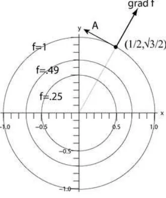
At any specific point (x, y), grad(f)is a vector that gives the direction of the maximum increase of the function f(x, y). Consider the following contour plot of the function f(x, y) =x2+y2
Figure 1.1. Contour plot of f(x, y) =x2+y2
Note that all points (x, y)on the circle labelled f= 1 have function value equal to 1. The point (x, y) = (1/2,√3/2)is one such point on the circle f= 1. Notice that if we change the (x, y)values in the direction of arrow A, that is if we take (x, y)values along the circle f = 1, then the function f(x, y)does not change value. In order to get the maximum increase in the functionf(x, y)we must move in the direction perpendicular to the circle f= 1; this is the direction specified by
grad(f) = 2xi+ 2yj
=i+ 3√ j
in the diagram.
Definition 1.27. Let (x, y) be a point on a curve C in the Cartesian plane R2 that has a well-defined tangent vector T. Then any vectornat the point(x, y)that is perpendicular to the tangent vectorT is called anormal vectorto the curveC at the point(x, y).
Example 1.28. In Figure 1.1 above, the arrowAis a tangent vector to the curvef= 1at the point (x, y) = (1/2,√3/2). The vector
grad(f) =i+ 3√ j
is an example of a normal vector to the curve f= 1at the point(1/2,√3/2).
Definition 1.29. Let f(x, y) be a function of two variables and let c be a constant. The set of points that satisfy
f(x, y) =c
Example 1.30. Letf(x, y) =x2+y2.Then the level curve f(x, y) = 1
is the circle
x2+y2= 1.
Notice that the three level curves f(x, y) = 1,f(x, y) =.49 and f(x, y) =.25 are shown in Figure 1.1 above.
Theorem 1.31. Letf(x, y) =c be a level curveC in the Cartesian plane wheref(x, y)is a differ-entiable function. Then if grad(f)at a point(x, y)is not the zero vector, then it is a normal vector to the curveC at the point(x, y).
Example 1.32. Find a normal vector to the ellipsex2+ 4y2= 1at the point 1 2 √ , 1
2 2√
.
Answer: Notice that the curve x2+ 4y2= 1is a level curve as it is in the form f(x, y) = 1
where f(x, y) =x2+ 4y2. The gradient of the functionf is
grad(f) =∂f ∂xi+
∂f ∂yj = 2xi+ 8yj
and at the point(x, y) = 1
2 √ , 1
2 2√
, grad(f)is equal to
grad(f) = 2xi+ 8yj
= 2
2
√ i+ 8 2 2√ j =√2i+ 2 2√ j
which, by Theorem 1.31 is a normal vector tox2+ 4y2= 1at the point 1 2 √ , 1
2 2√
.
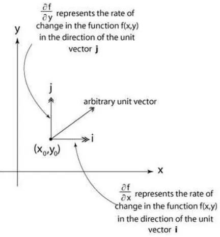
Recall that the partial derivative ∂f∂x(x0, y0)measures the rate at which the function f is increasing as thex-value increases while keeping the y−value fixed, in other words, ∂f∂x(x0, y0)gives the rate of change in the function f as the (x, y)points move from (x0, y0) in the direction of the horizontal unit vectori; see Figure 1.2 below.
Similarly the partial derivative ∂f
Figure 1.2. Diagram of the domain of the functionf
If we wish to determine the rate at which a function changes as the(x, y) points move from a fixed point (x0, y0) in the direction of a unit vector that is not horizontal or vertical, then we shall need the following definition.
Definition 1.33. The directional derivative of a function f(x, y) in the direction of a unit vectoruat a point(x0, y0), denoted asDuf, is defined as the dot product
Duf=u·grad(f)
Example 1.34. Find the directional derivative of the function f(x, y) =x2+y2 at the point(1,2) in the directioni−j.
Answer: In the definition of the directional derivative, the direction is specified by a unit vector. We first find the unit vectoruparallel toi−j
u= i−j length of i−j
= i−j
12+ (−1)2 p
= 1
2
√ i− 1
2
√ j
The vector grad(f)at the point(x, y) = (1,2)is
grad(f) =∂f ∂xi+
∂f ∂yj = 2xi+ 2yj
= 2i+ 4j
and the required directional derivative is
Duf=u·grad(f)
=
1 2
√ i− 1
2
√ j
·(2i+ 4j)
The gradient of a function f(x, y, z)of three variables is defined and has properties analogous to the gradient of a function of two variables.
Definition 1.35. If f(x, y, z) is a function of three variables, then the gradient of the function, denoted as grad(f), is the vector function defined as
grad(f) =∂f ∂xi+
∂f ∂yj+
∂f ∂zk.
Note that the vector differential operator of Definition 1.21 can be used to give an alternative expression of grad(f)
grad(f) =∇f .
Definition 1.36. Let f(x, y, z)be a function of three variabless and letc be a constant. The set of points that satisfy
f(x, y, z) =c
called alevel surfaceof the functionf(x, y, z).
Example 1.37. Letf(x, y, z) =x2+y2+z2.Then the level surfaceS
f(x, y, z) = 1 is the sphere
x2+y2+z2= 1. of radius1is illustrated in Figure 1.3 below.
Figure 1.3.
Definition 1.38. The tangent plane to a point P on a surface S is the plane that touches the surface at the pointP. Anormal vector to a surfaceS at the point P is a vector that is perpen-dicular to the tangent plane at the pointP.
Example 1.40. Find a normal vector to the spherex2+y2+z2= 1at the point(1,0,0). Answer: Notice that the surface x2+y2+z2= 1is in the form
f(x, y, z) = 1
where f(x, y, z) =x2+y2+z2. The gradient of the functionf is grad(f) =∂f
∂xi+ ∂f ∂yj+
∂f ∂zk = 2xi+ 2yj+ 2zk
and at the point(x, y) = (1,0,0), grad(f)is equal to
grad(f) = 2xi+ 2yj+ 2zk
= 2i+ 0j+ 0k
= 2i
which, by Theorem 1.39 is a normal vector to the sphere x2+y2+z2= 1at the point(1,0,0).
As in the case of a function of two variables, the partial derivatives ∂x∂f(x0, y0, z0), ∂f
∂y(x0, y0, z0)and ∂f
∂z(x0, y0, z0) measure the rate at which a function f(x, y, z) changes as the(x, y, z) points move from a fixed point (x0, y0, z0)in the direction of a unit vectorsi,j andkrespectively.
If we wish to determine the rate at which a function changes as the (x, y, z) points move from a fixed point (x0, y0, z0)in the direction of a unit vector that is not a standard unit vector i, j or k, then, as in the case of a function of two variables, we need the definition of a directional derivative.
Definition 1.41. The directional derivative of a function f(x, y, z) in the direction of a unit vectoruat a point(x0, y0, z0), denoted asDuf, is defined as the dot product
1.4 Line integrals and double integrals
1.4.1 Line integrals
Definition 1.42. LetF(x, y)be a continuous vector field defined on the Cartesian plane and letC be the smooth parametric curve
r(t) =x(t)i+y(t)j a6t6b. Then the line integral of the vector fieldF along the curveC is
Z
C
F·dr= Z
a b
F(x(t), y(t))·(x′(t)i+y′(t)j)dt
A line integral R
C F·dr can be interpreted as the work done on a particle by a force fieldF as it travels on a pathC. Consider the following example.
Example 1.43. LetF(x, y) = 3x2ibe a vector field on the Cartesian plane. Calculate the following line integrals
i. R
C1F·dr whereC1is the curve
r(t) = (1 +t)i+j 06t61
ii. R
C2F·dr whereC2is the curve
r(t) =i+ (1 +t)j 06t61.
Answer:
i.
Z
C1
F·dr= Z
a b
F(x(t), y(t))·(x′(t)i+y′(t)j)dt
= Z
0 1
F((1 +t),1)·((1 +t)′i+ (1)′j)dt
= Z
0 1
3(1 +t)2i
·(1i+ 0j)d t
= Z
0 1
3(1 +t)2dt
=
(1 +t)3 0 1
= 8. ii.
Z
C2
F·dr= Z
a b
F(x(t), y(t))·(x′(t)i+y′(t)j)dt
= Z
0 1
F(1,(1 +t))·((1)′i+ (1 +t)′j)dt
= Z
0 1
3(1)2i
·(0i+ 1j)dt
= Z
0 1
3i·(0i+ 1j)dt
= Z
0 1
0dt
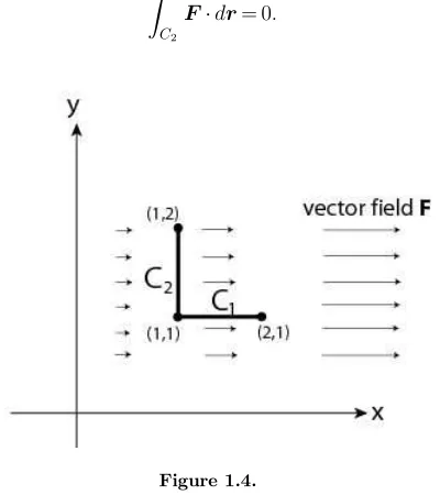
Figure 1.4 below is an illustration of the vector fieldF(x, y) = 3x2iand the two curves
C1: r(t) = (1 +t)i+j 06t61
C2: r(t) =i+ (1 +t)j 06t61.
If we regard the vector field F as a force field then as C1lies in the direction of F, we expect F to add energy to a particle travelling along the pathC1. This agrees with
Z
C1
F·dr= 8
in part i). However, the curve C2 is perpendicular to the direction of vector field and therefore F does not add any energy to a particle travelling alongC2which agrees with the answer
Z
C2
F·dr= 0. in part ii).
Figure 1.4.
The definition of a line integral in three dimensional space is similar to the definition in the Carte-sian plane.
Definition 1.44. LetF(x, y, z)be a continuous vector field defined in three dimensional space and letC be the smooth parametric curve
r(t) =x(t)i+y(t)j+z(t)k a6t6b. Then the line integral of the vector fieldF along the curveC is
Z
C
F·dr= Z
a b
F(x(t), y(t), z(t))·(x′(t)i+y′(t)j+z′(t)k)d t.
Example 1.45. Evaluate
Z
C
F·dr
whereF is the vector field in three dimensional space
F(x, y, z) =xyi+yzj+zxk
andC is the parametric curve
Answer: From Definition 1.44 above, we have
Z
C
F·dr= Z
a b
F(x(t), y(t), z(t))·(x′(t)i+y′(t)j+z′(t))dt
= Z
0 1
F(t, t2, t3)· (t)′i+ (t2)′j+ (t3)′k dt
= Z
0 1
t3i+t5j+t4k
· 1i+ 2tj+ 3t2k dt
= Z
0 1
(t3+ 2t6+ 3t6)dt =
t4
4+ 5t7
7
0 1
=27 28.
1.4.2 Path independence and conservative vector fields
Definition 1.46. If C is a parametric curve in the Cartesian plane of the form
r(t) =f(t)i+g(t)j where a6t6b,
then the initial point of C is given by the position vector r(a) and the terminal point of C is given by the position vectorr(b). Similarly, one can define the initial and terminal points of a
para-metric curve
r(t) =f(t)i+g(t)j+h(t)k a6t6b in three dimensional space.
Example 1.47. LetF be the vector field
F(x, y) =y2i+xj and letC1andC2be the parametric curves defined as
C1: r(t) = (5t−5)i+ (5t−3)j 06t61
C2: r(t) = (4−t2)i+tj −36t62.
a) Sketch the curvesC1andC2and verify thatC1, C2have the same initial and terminal point b) By evaluating the respective line integrals, show that
Z
C1
F·dr
Z
C2
F·dr .
Answer:
a) In the case of C1, we have
x= 5t−5 y= 5t−3.
Note that bothx, y are linear functions of tand that the parameter ttakes values in a finite interval 06t61.It follows thatC1is a line segment with initial pointr(0) = (−5,−3)and terminal pointr(1) = (0,2).
In the case ofC2, the initial point isr(−3) = (−5,−3)and terminal pointr(2) = (0,2). To determine the shape ofC2, we eliminatetfrom
x= 4−t2 y=t to obtain
It follows thatC2 is a segment of the parabolax= 4−y2that has initial point (−5,−3)and terminal point(0,2).
Figure 1.5. Sketch of curvesC1andC2
b) Using the definition of the line integral, we have
Z
C1
F·dr= Z
a b
F(x(t), y(t))·(x′(t)i+y′(t)j)dt
= Z
0 1
F((5t−5),(5t−3))·((5t−5)′i+ (5t−3)′j)dt
= Z
0 1
(5t−3)2i+ (5t−5)j
·(5i+ 5j)d t
= Z
0 1
5(5t−3)2+ 5(5t−5) dt
= 5 Z
0 1
25t2−25t+ 4 dt
=−56
and
Z
C2
F·dr= Z
a b
F(x(t), y(t))·(x′(t)i+y′(t)j)dt
= Z
−3 2
F((4−t2), t)· (4−t2)′i+ (t)′j dt
= Z
−3 2
t2i+ (4−t2)j
·((−2t)i+j)d t
= Z
−3 2
(−2t)t2+ 4−t2 dt
= Z
−3 2
−2t3−t2+ 4 dt
=245 6 and clearly
Z
C1
F·dr
Z
C2
F·dr.
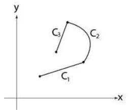
of smooth curvesC1, C2,, Cnsuch that the terminal point ofCiis the initial point ofCi+1.
Figure 1.6. A piecewise smoothC=C1∪C2∪C3
A line integral along a piecewise smooth curve is obtained by adding the line integrals of its indi-vidual pieces.
Definition 1.49. LetC=C1∪C2∪ ∪Cn be a piecewise smooth curve. Then the line integral of
the vector fieldF along the curveC is
Z
C
F·dr= Z
C1
F·dr+ Z
C2
F·dr++
Z
Cn
F·dr
Definition 1.50. A line integral
Z
C
F·dr
is said to beindependent of pathif Z
C
F·dr= Z
C′
F·dr
for any piecewise smooth curve C′which has the same initial point and terminal point as the curve C.
Example 1.51. Consider curvesC1, C2and the line integral Z
C1
F·dr
as defined in Example 1.47. This line integral is notindependent of path as C2has the same initial and terminal points as C1but
Z
C1
F·dr
Z
C2
F·dr.
Recall from Remark 1.25 that the gradient grad(f)of a functionf(x, y)is in fact a vector field.
Definition 1.52. Let F be a vector field defined on Rn1.2. Then F is said to be a conservative vector field if there exists a function f such that
F=grad(f).
For such a case, f is called apotential functionfor the vector fieldF. 1.3
1.2. In this class we consider only the cases ofn= 2(the Cartesian plane) andn= 3(three dimensional space)
The above is the standard definition of a conservative vector field; however it is not a practical method of determining whether or not a vector field is conservative. A more useful criterion for vector fields inR2is the following
Theorem 1.53. Let
F(x, y) =P(x, y)i+Q(x, y)j.
be a vector field defined onR2where the component functions P and Qhave continuous first partial derivatives.ThenF is conservative if and only if
∂P ∂y=
∂Q ∂x.
Example 1.54. Show that the vector field
F(x, y) = (6x+ 5y)i+ (5x+ 4y)j
is conservative and determine a potential function for F(x, y).
Answer: In this case
P(x, y) = 6x+ 5y Q(x, y) = 5x+ 4y and
∂P ∂y= 5 =
∂Q ∂x
so it follows thatF is conservative. Let f be a potential function forF. Then
grad(f) =F
⇒∂x∂fi+∂f
∂yj= (6x+ 5y)i+ (5x+ 4y)j
⇒
∂f
∂x= 6x+ 5y ∂f
∂y= 5x+ 4y
. (1.2)
Using partial integration1.4to integrate the first equation of (1.2) with respect tox, we have
f(x, y) = 3x2+ 5xy+C(y). (1.3)
The function C(y)can be determined by differentiating equation (1.3) with respect to y and using the second equation of (1.2)
∂f
∂y= 5x+C′(y) = 5x+ 4y
⇒C′(y) = 4y
⇒C(y) = 2y2+K whereK is a constant of integration. We therefore have
f(x, y) = 3x2+ 5xy+ 2y2+K
and by choosing K= 0 we have that f= 3x2+ 5x y+ 2y2 is a potential function for the vector field
F.
The following result specifies exactly what conditions are required for a line integral in Rn to be independent of path.
Theorem 1.55. LetF be a vector field onRn. Then the line integral Z
C
F·dr
is independent of path if and only if F is a conservative vector field.
Furthermore, the value of a line integral that is independent of path can be determined from the endpoints of the curve and a potential function of the vector field
Theorem 1.56. (Fundamental Theorem of Line Integrals) LetF be a vector field defined on Rnand R
C F·dr be a line integral that is independent of path. Then Z
C
F·dr=f(r2)−f(r1)
where f is a potential function for the the vector field F and r1, r2 are respectively the initial and terminal points of the curveC.
Example 1.57. LetF be the vector field
F(x, y, z) =x3y4i+x4y3j and letC be the parametric curve defined as
C: r(t) =√ti+ (1 +t3)j 06t61. a) Show thatF is a conservative vector field
b) Find a potential function forF
c) Use the potential function of part (b) to evaluate the line integral R
CF·dr. Answer:
a) The given vector field is of the formF=P(x, y)i+Q(x, y)jwhere
P(x, y) =x3y4
Q(x, y) =x4y3. As
∂P ∂y= 4x
3y3=∂Q
∂x so it follows thatF is conservative.
b) Letf be a potential function forF. Then
grad(f) =F
⇒∂x∂fi+∂f ∂yj=x
3y4i+x4y3j
⇒
∂f ∂x=x
3y4
∂f ∂y=x
4y3
. (1.4)
By partially integrating the first equation of (1.4) with respect tox, we have
f(x, y) =x
4y4
4 +C(y). (1.5)
The functionC(y)can be determined by differentiating equation (1.5) with respect to y and using the second equation of (1.2)
∂f ∂y=x
4y3+C′(y) =x4y3
⇒C′(y) = 0
whereK is a constant of integration. We have
f(x, y) =x
4y4
4 +K
and by choosingK= 0we have thatf=x44y4 is a potential function for the vector fieldF. c) Using the parametric definition of C, we have that the initial and terminal points of C are
r1=r(0) = (0,1)
r2=r(1) = (1,2) and from Theorem 1.56
Z
C
F·dr=f(r2)−f(r1)
=f(1,2)−f(0,1)
=1
424
4 −
0414 4 = 4.
1.4.3 Double integrals
We give the definition of a double integral over a rectangular regionRand then state a theorem that gives a procedure for evaluating double integrals over a rectangular region. We then note that a double integral may be interpreted as a volume. Finally we explain the evaluation of double inte-grals over TypeI, TypeII and circular regions.
Definition 1.58. LetRbe a rectangular region in the Cartesian plane defined by R={(x, y)|a6x6b, c6y6d}.
Divide the rectangular regionRinto subrectangles by partitioning the intervalsa6x6b and c6y6
d :
a=x0< x1< < xm=b
c=y0< y1<< yn=d
and define the subrectangle Rij as
Choose points (xij∗, yij∗) in each subrectangleRij. Let ∆Aij denote the area of the subrectangle Rij and let
P
denote the length of the largest diagonal of all subrectangles (note that as we take smaller subrectangles of Rwe have that
P
→0). Then thedouble integral of the functionf(x, y)over the rectangular regionRis defined to be the limit
Z Z
R
f(x, y)dA= lim kPk→0
X
i=1 m
X
j=1 n
f(xij∗, yij∗)∆Aij
if this limit exists.
The above definition is not usually used to evaluate double integrals. We shall give a method of eval-uating double integrals based on the following procedure ofpartial integration.
Example 1.59. (of partial integration)
Z
1 2
xy dy=
xy2 2
y=1 y=2
=x2
2
2 −
x12 2 =3x
2 .
Notice in the above procedure of partial integration we
• integrate a function of two variables with respect to y
• treatxas a constant when integrating
• the answer
Z
1 2
xy dy=3x 2 is a function of x.
We can also integrate partially with respect tox:
Example 1.60.
Z
3 4
cos(xy)dy=
sin(xy) y
x=3 x=4
=sin(4y)
y −
sin(3y) y
and notice in this case our answer is a function of y.
Using the procedure of partial integration and the following theorem we can evaluate double inte-grals over rectangular regions.
Theorem 1.61. (Fubini’s Theorem) If the function f(x, y)is continuous at each point in a rect-angular region
R={(x, y)|a6x6b, c6y6d} then
Z Z
R
f(x, y)dA= Z
a b Z
c d
f(x, y)dy !
dx= Z
c d Z
a b
f(x, y)dx !
dy. (1.6)
Note that the integrals within the brackets of (1.6) are evaluated by partial integration. Also notice that (1.6) implies that the double integral over a rectangular region can be obtained by integrating with respect to yand thenxor integrating with respect toxand theny.
Example 1.62. Evaluate the double integral Z Z
R
whereRis the rectangular region
R={(x, y)|06x63,16y62}.
Answer: By Fubini’s Theorem Z Z
R
x2y dA= Z
0 3 Z
1 2
x2ydy
dx
= Z
0 3
x2y2 2
y=1 y=2
dx
= Z
0 3
x222
2 −
x212
2
dx
= Z
0 3 3
x2 2 dx
=
x3 2
x=0 x=3
=27 2 .
Notation 1.63.
i. The integral
Z
a b Z
c d
f(x, y)dy !
dx
is usually denoted as
Z
a bZ
c d
f(x, y)dydx.
ii. Similarly, the integral
Z
c d Z
a b
f(x, y)dx !
dy
is usually denoted as
Z
c dZ
a b
f(x, y)dxdy.
Recall that the graph of a function f(x, y)forms a surface in three dimensional space. Given a func-tion f(x, y)>0for each point(x, y)in a rectangular domainR, then the double integral
Z Z
R
f(x, y)dA
We now consider double integrals over regions in the Cartesian plane that are not rectangular.
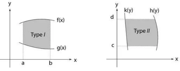
Definition 1.64.
i. AType I region is a region in the Cartesian plane that may be described as
R={(x, y)|a6x6b, f(x)6y6g(x)}
wheref(x)and g(x)are continuous functions of x.
ii. AType II region is a region in the Cartesian plane that may be described as
R={(x, y)|k(y)6x6h(y), c6y6d}
wherek(y)andh(y)are continuous functions of y.
Figure 1.7.
As in the evaluation of a double integral over a rectangular region, evaluating double integrals over Type I and Type II regions requires the use of partial integration. Note that for a Type I region,
the integration is done with respect to the y variable first and then with respect toxvariable. For a Type II region, the integration is done with respect to they variable first and then with respect tox
variable.
Theorem 1.65.
i. If the functionf(x, y)is continuous at each point in a TypeI region
R={(x, y)|a6x6b, g(x)6y6f(x)}
then
Z Z
R
f(x, y)dA= Z
a b Z
g(x) f(x)
f(x, y)dy !
dx
ii. If the functionf(x, y)is continuous at each point in a TypeII region
R={(x, y)|k(y)6x6h(y), c6y6d} then
Z Z
R
f(x, y)dA= Z
c d Z
k(y) h(y)
f(x, y)dx !
Example 1.66. Evaluate the double integral
Z Z
R
x dA
whereR={(x, y)|06x61,06y6p1−x2
}.
Answer: Notice thatRis a TypeI region. Then
Z Z
R
xd A= Z
0 1 Z
0 1−x2
√
x dy !
d x
= Z
0 1
[xy]y=0y= 1−x2 √
dx
= Z
0 1
xp1−x2−x(0)dx =
Z
0 1
xp1−x2d x
= "
−(1−x
2)32
3 #
x=0 x=1
=1 3.
Example 1.67. Evaluate the double integral
Z Z
R
xy dA
whereR is the region bounded by the linex=y+ 1and the parabolax=y
2
2 −3.
Answer: By solving the equations
x=y+ 1
x=y
2
2 −3
⇒ y+ 1 =y
2
2 −3 ⇒ y=−2,4
and we see that the linex=y+ 1and the parabolax=y
2
From the above diagram we can writeRas
R={(x, y)|y
2
2 −36x6y+ 1, −26y64} and so the regionRis of TypeII. Then
Z Z
R
xy dA= Z
−2 4
Z
y2
2−3 y+1
xy dx
dy
= Z
−2 4
x2y
2
x=y 2 2−3 x=y+1
dy
=1 2 Z
−2 4
(y+ 1)2y−
y2 2 −3
2 y
! dy
=1 2 Z
−2 4
y3+ 2y2+y−y
5
4 + 3y
3−9y
dy
=1 2 Z
−2 4
−y
5
4 + 4y
3+ 2y2−8y
dy
=36.
Some regions in the Cartesian plane are more easily described by the use of polar coordinates.
Definition 1.68. Apolar rectangle is a region in the Cartesian plane that may be described in polar coordinates(r, θ)as
R={(r, θ)|θ16θ6θ2, a6r6b} whereaandbare real constants such that06a < b.
Figure 1.8.
Example 1.69. Express the following region
R={(x, y)|96x2+y2625, x>0, y>0}
as a polar rectangle.
Answer: The equations
x2+y2= 9 x2+y2=25
describe circles of radius3 and5 respectively that have the origin as center. Therefore the inequali-ties
describe points that lie between the circles and in the first quadrant
and so we can writeRas a polar rectangle
R={(r, θ)|06θ6π
2, 36r65}.
We shall use the following theorem to evaluate double integrals over regions in the Cartesian plane that are polar rectangles. Notice that the following theorem is a conversion of a double integral in xy−coordinates to a double integral in polar coordinates.
Theorem 1.70. If the functionf(x, y)is continuous at each point in a polar rectangle
R={(r, θ)|θ16θ6θ2, a6r6b} then
Z Z
R
f(x, y)dA= Z
θ1
θ2 Z
a b
f(rcosθ, rsinθ)rdr !
dθ.
Example 1.71. Evaluate the following double integral
Z Z
R
1−(x2+y2) dA
whereR={(x, y)| 06x2+y261} by converting to polar coordinates.
Answer: The regionRis the unit disc
and so we can writeRas a polar rectangle
From Theorem 1.70, we have
Z Z
R
1−(x2+y2) dA=
Z
0 2π Z
0 1
(1−(r2cos2θ+r2sin2θ))rdr
dθ
= Z
0 2π Z
0 1
(1−r2)rdr
dθ
= Z
0 2π Z
0 1
(r−r3)dr
dθ
= Z
0 2π
r2
2 −
r4 4
0 1
dθ
= Z
0 2π 1
4dθ =π
2.
1.5 Green’s theorem
Definition 1.72.
i. A parametric curveC is calledclosedif its terminal point coincides with its initial point. ii. Asimple curveC is a curve that does not intersect itself anywhere between its endpoints.
Figure 1.9. Examples of curves
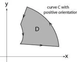
Convention:A positive orientation of a simple closed curveC refers to a counterclockwise traversal of C.
Theorem 1.73. (Green’s Theorem) Let C be a positively oriented, piecewise smooth, simple closed curve in the Cartesian plane. LetDbe the region bounded byC. LetF be the vector field
F(x, y) =P(x, y)i+Q(x, y)j
where P(x, y) and Q(x, y) have continuous partial derivatives on an open region that containsD. Then
Z
C
F·dr= Z Z
D
∂Q ∂x−
∂P ∂y
Figure 1.10. RegionDbounded by curveC
Note that Green’s Theorem states that the line integral around a simple closed curve C may be obtained by evaluating a double integral over the regionDenclosed byC.
Example 1.74. LetC=C1∪C2∪C3be the simple closed curve
enclosing the triangular regionD. Use Green’s Theorem to determine the line integral Z
C
(x4i+xyj).dr (1.7)
by evaluating an appropriate double integral.
Answer: By Green’s Theorem Z
C
F·dr= Z Z
D
∂Q ∂x−
∂P ∂y
dA
we have that the line integral (1.7) is equal to a double integral
Z
C
(x4i+xyj)·dr= Z Z
D
∂ ∂x(xy)−
∂ ∂y(x
4)
dA
= Z Z
D
(y−0)dA
= Z Z
D
y dA
(1.8)
that is, we can describe the regionDas the set
D={(x, y)|06x61,06y61−x}
and therefore
Z Z
D
y dA= Z
0 1Z
0 1−x
y dy dx (1.9)
Substituting (1.9) into (1.8) we have
Z
C
(x4i+xyj)·dr= Z Z
D
y dA
= Z
0 1Z
0 1−x
y dy dx
and notice that this is the point of Green’s theorem – for a simple closed curve C, a line integral aroundC is equal to a double integral over the region enclosed byC
Z
C
(x4i+xyj).dr= Z
0 1Z
0 1−x
y dy dx
and we can evaluate this double integral by using partial integration
Z
C
(x4i+xyj).dr= Z
0 1Z
0 1−x
y dy d x
= Z
0 1
y2 2
y=0 y=1−x
dx
= Z
0 1 (1
−x)2
2 dx
=
−(1−x)
3
6
0 1
=1 6
1.6 Surface integrals
1.6.1 Parametric surfaces
Recall that some curvesC in three dimensional space can be described parametrically
C: r(t) =x(t)i+y(t)j+z(t)k a6t6b,
may be written parametrically as
r(t) =ti+tj+ (1−t)k 06t61.
We now describe surfaces in three dimensional space by the use of vector functions r(u, v) of two parametersuandv.
Definition 1.75. Aparametric surfaceS in three dimensional space is obtained by specifyingx, y andzto be continuous functions of parametersuandv
x=f(u, v) y=g(u, v) z=h(u, v)
where (u, v)∈R and R is a region in the u v−plane. The parametric surfaceS can be written in vector form
r(u, v) =f(u, v)i+g(u, v)j+h(u, v)k (u, v)∈R.
Example 1.76. LetS be the (truncated) plane defined by y= 1, 06x, z61.
Then we can describeSa parametric surface by
r(u, v) =ui+j+vk (u, v)∈R.
whereRis the region{(u, v)|06u, v61}
in theuv−plane. Notice that each point(u, v)of Rdefines a unique point inS.
Example 1.77. Describe the cylinderS
Answer: We can use polar coordinates to describe the cylinderS
as the parametric surface
r(θ, z) = 2cosθi+ 2sinθj+zk (θ, z)∈R
whereRis the region{(θ, z)|06θ62π,06z63}
in theθz−plane.
Lemma 1.78. LetSbe a parametric surface
r(u, v) =f(u, v)i+g(u, v)j+h(u, v)k (u, v)∈R
that is smooth. Then anormal vectorn toS at the pointr(u0, v0)is given by
n=ru×rv whereruandrv are the vectors
ru=∂f
∂u(u0, v0)i+ ∂g
∂u(u0, v0)j+ ∂h
∂u(u0, v0)k
rv=∂f
∂v(u0, v0)i+ ∂g
∂v(u0, v0)j+ ∂h
∂v(u0, v0)k provided that ru×rv0.
Example 1.79. Find a normal vector to the cylinder
S: r(θ, z) = 2cosθi+ 2sinθj+zk (θ, z)∈R (1.10)
whereRis the region{(θ, z)|06θ62π,06z63} at the point(2,0,0).
Answer: In this case the parameters are θandz.Note that the point(2,0,0)corresponds to(θ, z) = (0,0)as
r(0,0) = 2cos0i+ 2sin0j+ 0k
The vector functions rθ(θ, z)andrz(θ, z)are obtained by differentiating (1.10) partially with respect toθandz respectively
rθ(θ, z) =−2sinθi+ 2cosθj+ 0k
rz(θ, z) = 0i+ 0j+ 1k and at(θ, z) = (0,0)
rθ(0,0) = 2j
rz(0,0) =k
and the normal vector at the point (2,0,0)is
n=rθ(0,0)×rz(0,0)
= 2j×k
= 2i
1.6.2 Surface integrals
Definition 1.80. LetS be a smooth parametric surface
r(u, v) =x(u, v)i+y(u, v)j+z(u, v)k (u, v)∈R
whereRis a region in theu v−plane and letf(x, y, z)be a continuous function defined onS. Then thesurface integralof the functionf(x, y, z)over the surfaceSis
Z Z
S
f(x, y, z)dS= Z Z
R
f(x(u, v), y(u, v), z(u, v))|ru×rv|dA (1.11)
Note that equation (1.11) defines a surface integral to be equal to a double integral over a region R in theuv−plane whereuandvare the parameters of the surfaceS.
Example 1.81. Evaluate the surface integral Z Z
S
(x2y+z2)dS
Answer: Our definition (1.11) of a surface integral requires that the surfaceS
be given in parametric form:
S: r(θ, z) = 3cosθi+ 3sinθj+zk (θ, z)∈R (1.12)
whereRis the region {(θ, z)|06θ62π,06z62}. Note in this case we use the parametersr andθ instead of uandv. Thex, yandz components ofSare
x= 3cosθ y= 3sinθ z=z. The vectorsrθandrzare
rθ=
∂x ∂θi+
∂y ∂θj+
∂z
∂θk=−3sinθi+ 3cosθj+ 0k
rz=∂x
∂zi+ ∂y ∂zj+
∂z
∂zk= 0i+ 0j+k and we have
rθ×rz= (−3sinθi+ 3cosθj)×k
=
i j k
−3sinθ 3cosθ 0
0 0 1
= 3cosθi+ 3sinθj
and therefore
|rθ×rz|=|3cosθi+ 3sinθj|
= 9√ cos2θ+ 9sin2θ
= 3.
From the definition of a surface integral
Z Z
S
(x2y+z2)dS= Z Z
R
f(x(θ, z), y(θ, z), z(θ, z))|rθ×rz|d A
= Z Z
R
(3cosθ)2(3sinθ) +z2 3dA
= 3 Z Z
R
27cos2θsinθ+z2 dA
in theθz−plane.Therefore
Z Z
S
(x2y+z2)dS= 3 Z Z
R
27cos2θsinθ+z2 dA
= 3 Z
0 2πZ
0 2
27cos2θsinθ+z2 dzdθ
= 3 Z
0 2π
27cos2θsinθz+z3
3
0 2
dθ
= 3 Z
0 2π
54cos2θsinθ+8
3
dθ
= 3
−54cos
3θ
3 +
8θ 3
0 2π
(use substitutionu=cosθ)
=16π
A surface integral of a function f over a surfaceS can be interpreted as follows. Suppose that a sur-face Sis subdivided intonsmaller surfacesSi.
Choose a point (xi∗, yi∗, zi∗)on each smaller surface Si. Let ∆Aibe the area of the small surface Si and multiply this area by the value f(xi∗, yi∗, zi∗)of the functionf at the point(xi∗, yi∗, zi∗). Hence we have a ‘weighted’ area
f(xi∗, yi∗, zi∗)∆Ai
for each of the nsmaller surfacesSiof the entire surface S. Then the surface integral of the function
f over the surfaceSis approximately the sum of each of the weighted areas for theSi
Z Z
S
f(x, y, z)dS≃X
i=1 n
f(xi∗, yi∗, zi∗)∆Ai (1.13)
and if the number nof smaller surfaces Sigets larger then the approximation (1.13) gets better, so we have
Z Z
S
f(x, y, z)dS= lim n→∞
X
i=1 n
f(xi∗, yi∗, zi∗)∆Ai. (1.14)
Notice that if the functionf(x, y, z) = 1then from (1.14) we have
Z Z
S
1dS= lim n→∞
X
i=1 n
∆Ai
Lemma 1.82. The surface integral of the constant functionf= 1 over the surfaceSis equal to the surface area of S
Z Z
S
1d S=surface area ofS.
Example 1.83. Find the surface area of the truncated planeS
r(u, v) =ui+j+vk (u, v)∈R.
whereRis the region{(u, v)|06u, v61}.
Answer: The surfaceS is shown in the following diagram
(see Example 1.76). Clearly the surface area of S is equal to 1; let us verify this by evaluating the surface integral
Z Z
S
1dS.
Thex, yandzcomponents ofS are
x=u y= 1 z=v.
The vectorsruandrvare
ru=
∂x ∂ui+
∂y ∂uj+
∂z
∂uk=i+ 0j+ 0k
rv=
∂x ∂vi+
∂y ∂vj+
∂z
∂vk= 0i+ 0j+k and we have
ru×rv=i×k
=
i j k
1 0 0 0 0 1 =−j
and so
|ru×rv|=| −j|= 1
From the definition of a surface integral
Z Z
S
1ds= Z Z
R
1|ru×rv|dA
= Z Z
R
This last integral is a double integral of the function f(u, v) = 1 over the rectangular regionR
in theuv−plane.Therefore
Z Z
S
1dS= Z Z
R
1dA
= Z
0 1Z
0 1
1dudv
= Z
0 1
[u]01d v =
Z
0 1
(1−0)dv
= Z
0 1
1dv
= 1
which agrees with our expected answer.
Recall that the graph of a function g(x, y)forms a a surface in three dimensional space. LetRbe a region in thexy−plane and letS be the surface formed as the image of the regionRin the graph of g(x, y):
Then the following lemma expresses a surface integral of a function f(x, y, z)over such a surfaceS in terms of the function g(x, y).
Lemma 1.84. LetRbe a region in the x y−plane and letS be the image of Rin the graph of a function g(x, y). Then the surface integral of the functionf(x, y, z)over the surfaceS is equal to a double integral over the regionRin thexy−plane:
Z Z
S
f(x, y, z)dS= Z Z
R
f(x, y, g(x, y)) 1 +
∂g ∂x
2 +
∂g ∂y
2 s
d A
Proof. The surfaceS can be written parametrically as
with parametersxand y. The vectorsrxandryare
rx=
∂ ∂x(x)i+
∂ ∂x(y)j+
∂
∂x(g(x, y))k=i+ 0j+ ∂g ∂xk
ry= ∂
∂y(x)i+ ∂ ∂y(y)j+
∂
∂y(g(x, y))k= 0i+j+ ∂g ∂yk and therefore
rx×ry=
i+∂g ∂xk
×
j+∂g ∂yk =
i j k
1 0 ∂g∂x
0 1 ∂g∂y
=−∂x∂gi−∂g
∂yj+k
hence
|rx×ry|= −
∂g ∂xi−
∂g ∂yj+k
= 1 +
∂g ∂x 2 + ∂g ∂y 2 s
and from the parametric definition of a surface integral in Definition 1.80 we have
Z Z
S
f(x, y, z)dS= Z Z
R
f(x, y, g(x, y))|rx×ry|dA
= Z Z
R
f(x, y, g(x, y)) 1 + ∂g ∂x 2 + ∂g ∂y 2 s dA
which is the desired result.
Example 1.85. Find the surface area of the hemisphere of radiusa
z=pa2−(x2+y2)
.
Answer: Denote the hemisphere asS
Notice that the hemisphereS is the image of the regionR
R: x2+y26a2 in the graph of the function
z=g(x, y) =pa2−(x2+y2)
Recall from Lemma 1.82 that the surface area of S is given by the surface integral of the constant functionf= 1overS, that is
surface area ofS= Z Z
S
1dSs.
Now because the hemisphereS is the image of a regionRin the graph of the function g(x, y), from Lemma 1.84 we have
Z Z
S
1dS= Z Z R 1 + ∂g ∂x 2 + ∂g ∂y 2 s dA
and therefore we have
surface area ofS= Z Z
S
1d S
= Z Z R 1 + ∂g ∂x 2 + ∂g ∂y 2 s dA = Z Z R
1 + x
a2−(x2+y2) p
!2
+ y
a2−(x2+y2) p !2 v u u t dA = Z Z R
1 + x
2+y2
a2−(x2+y2) s dA = Z Z R a2
a2−(x2+y2) s
dA
=a Z Z
R
a2−(x2+y2)−12dA
whereR:x2+y26a2 is the disc of radiusa
and so we convert to polar coordinates
surface area ofS=a Z Z
R
a2−(x2+y2)−
1 2d A
=a Z 0 2πZ 0 a
a2−(r2cos2θ+r2sin2θ)−12rdrdθ
=a Z
0 2π Z
0 a
a2−r2−12rdr
dθ =a Z 0 2π
− a2−r212 r=0 r=a dθ =a Z 0 2π a dθ
= 2πa2
1.6.3 Surface integrals over vector fields
Definition 1.86. A surfaceS is called an orientable surfaceif there exists a continuous function
Anoriented surfaceSis a surface together with one of the two possible choices of orientation.
Example 1.87. LetSbe the cylinder
S: r(θ, z) = 2cosθi+ 2sinθj+zk (θ, z)∈R
where R is the region {(θ, z)|0 6 θ 6 2π, 0 6 z 6 3} defined in Example 1.79. Recall from that example, the vector
rθ(θ, z)×rz(θ, z) = (−2sinθi+ 2cosθj)×k
=
i j k
−2sinθ 2cosθ 0
0 0 1
= 2cosθi+ 2sinθj
is a normal vector at any pointr(θ, z)onS. The functionn(θ, z)given by
n(θ, z)= rθ×rz
|rθ×rz|
= 2cosθi+ 2sinθj 4cos2θ+ 4sin2θ
√
=cosθi+sinθj
assigns the unit normal vector cosθi+sinθj to each point on the cylinderS. Therefore
n(θ, z) =cosθi+sinθj
is an example of an orientation on the surfaceS. Notice that
n1(θ, z) =−n(θ, z) =−(cosθi+sinθj)
is the other possible orientation of the cylinderS.
We now define the surface integral over a vector field.
Definition 1.88. IfF(x, y, z)is a continuous vector field defined on a smooth parametric surfaceS
r(u, v) =x(u, v)i+y(u, v)j+z(u, v)k (u, v)∈R
whereRis a region in theuv−plane. LetShave an orientationngiven by
n= ru×rv
|ru×rv|
.
Then thesurface integralof the vector fieldF(x, y, z)over the surfaceS is Z Z
S
F.ndS= Z Z
R
F(x(u, v), y(u, v), z(u, v))·(ru×rv)dA. (1.15)
Example 1.89. Evaluate the surface integral
Z Z
S
(2xi+ 3xzj+y2k)·ndS whereSis the truncated plane1.5
r(u, v) =ui+j+vk (u, v)∈R
andRis the region{(u, v)|06u, v61}.
Answer: Thex, yandzcomponents ofS are
x=u y= 1 z=v.
The vectorsruandrvare
ru=∂x
∂ui+ ∂y ∂uj+
∂z
∂uk=i+ 0j+ 0k
rv=∂x
∂vi+ ∂y ∂vj+
∂z
∂vk= 0i+ 0j+k and we have
ru×rv=i×k
=
i j k
1 0 0 0 0 1 =−j
In this case the vector field F is
F(x, y, z) = 2xi+ 3xzj+y2k
From the definition of a surface integral of a vector field over a surface
Z Z
S
(2xi+ 3xzj+y2k).ndS= Z Z
R
F(x(u, v), y(u, v), z(u, v)).(ru×rv)dA
= Z Z
R
(2ui+ 3uvj+ 12k).(−j)dA
= Z Z
R −
3uv dA
This last integral is a double integral of the function f(u, v) =−3uv over the rectangular regionR
in theuv−plane.Therefore
Z Z
S
(2xi+ 3xzj+y2k).ndS= Z Z
R−
3uv dA
= Z
0 1 Z
0 1
−3uv dudv
= Z
0 1
−3u2v 2
0 1
dv
= Z
0 1
−3(1)2v
2 −
−3(0)2v
2
dv
= Z
0 1
−3v 2 d v
=−3 4
If the vector field F represents the velocity of a fluid moving in three dimensional space, then the surface integral of the vector field F over the surface S R R
S F.nd S can be interpreted as the volume of fluid flowing through the surfaceSin unit time. Consider the following example.
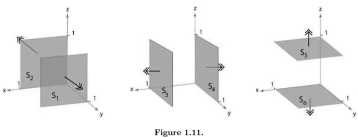
Example 1.90. Let F(x, y, z) =yj be a vector field in three dimensional space. Evaluate the fol-lowing surface integrals
i. R R
S1F.ndS whereS1is the parametric surface
r(u, v) =i+uj+vk (u, v)∈R.
whereRis the region{(u, v)|06u, v61}
ii. R R
S2F.ndS whereS2is the parametric surface
r(u, v) =vi+j+uk (u, v)∈R.
whereRis the region{(u, v)|06u, v61}.
Answer:
i. Note that the vector field F(x, y, z) =yj is in the direction of j at each point(x, y, z)in three dimensional space. The surfaceS1is the truncated plane shown in the diagram below
and noticeS1is parallel to the vector fieldF. If we regardF as the velocity of a fluid and as R R
S1 F.nd S can be interpreted as the volume of fluid flowing through the surfaceS1 in
unit time, we expect
Z Z
S1
as there is no fluid flowing throughS1 (only along S1). We verify this answer: thex, y andz components ofS1are
x= 1 y=u z=v. The vectorsruandrvare
ru=
∂x ∂ui+
∂y ∂uj+
∂z
∂uk= 0i+j+ 0k
rv=
∂x ∂vi+
∂y ∂vj+
∂z
∂vk= 0i+ 0j+k and we have
ru×rv=j×k
=
i j k
0 1 0 0 0 1 =i
and by therefore the surface integral of the vector fieldF over the surfaceS1is Z Z
S1
F.ndS= Z Z
R
F(x(u, v), y(u, v), z(u, v)).(ru×rv)dA
= Z Z
R
(uj)·idA
=