Vol. 2, No. 2, 2015
Manuscript History:
Received 28 March, 2015, Revised 1 August, 2015, Accepted 13 August, 2015, Published 30 September, 2015
Development and Demonstration of Graphical User Interface Spectrum
Sensing Algorithm using some Wireless Systems in South Africa
Jide Julius Popoola
1,2and Rex van Olst
31
Departmrnt of Electrical and Electronics Engineering, Federal University of Technology,
Akure, Nigeria.
2,3
School of Electrical and Information Engineering, University of the Witwatersrand,
Johannesburg, South Africa.
1,2
Email: [email protected]; [email protected],
3Email: [email protected]
Abstract
The wireless communication industry using radio spectrum is recently going through major innovations and advancements. With this transformation, the demand for and usage of radio spectrum has increased exponentially making radio spectrum indeed a scarce natural resource. In order to solve this problem, the possibility of opening up the unused portions of licensed spectrum by sharing using cognitive radio technology has been in the spotlight for maximizing radio spectrum utilization as well to as ensure sufficient radio spectrum availability for future wireless services and applications. With this objective in mind, this paper looks at the principles and technologies of cooperative spectrum sensing in cognitive radio environment in improving radio spectrum utilization. The paper provides a comprehensive review on spectrum sensing as a key functional requirement for cognitive radio technology by focusing on its application on dynamic spectrum access that enables unused portions of licensed spectrum to be used in an opportunistic manner as long as the operation of the unlicensed user will not affect that of the licensed user. In satisfying this dynamic spectrum access requirement, a friendly interactive graphical user interface (GUI) spectrum sensing application program was developed. The detail activities involve in the development of the application program, also known as spectrum sensing and detection algorithm (SSADA), was fully documented and presented in the paper. The developed graphical user interface application program after successfully developed was evaluated. The performance evaluations of developed graphical user interface sensing algorithm show that the algorithm performs favourably well. The program overall evaluation results provide bedrock information on how to improve cooperative spectrum sensing gain without incurring a cooperative overhead.
Keywords: Radio Spectrum, Dynamic Radio Access, Cognitive Radio, Spectrum Sensing, Spectrum Sensing and Detection Algorithm.
1. Introduction
Hence, as a public resource, radio spectrum is being managed by governments to ensure that it is shared equitably to promote the public interest, convenience, or necessity [2]. It is therefore being tightly regulated around the world by both the international and national regulators. The primary tool of spectrum management by government is a licensing system. This involves spectrum being apportioned into blocks for specific uses, and assigned licenses for these blocks to specific users. This “divideandset aside” policy grants exclusive right to use the assigned spectrum to licensed users on a long-term basis.
The main advantage of the licensing approach is that the licensee completely controls its assigned spectrum and can thus unilaterally manage interference between its users and their quality of service. However, there has recently been numbers of identifying disadvantages of traditional “once and for all” means of allocation of radio spectrum. The first observed disadvantage of this policy is the impossibility of re-allocating spectrum to different technologies or other users who might have better use for the spectrum [3]. The second observed disadvantage of the approach according to the authors in [3] is that the allocation procedures were lengthy and bureaucratic, opening up the possibility that the decision-making process could be influenced by non-relevant factors.
Furthermore, the “once and for all” or fixed allocation of radio spectrum that gives exclusive right of using the spectrum to the licensed owners has been observed as the main cause of both spectrum underutilization and spectrum artificial scarcity currently experiencing worldwide [4,5]. This has also been observed by some radio spectrum regulatory bodies such as Office of Communications (Ofcom) in United Kingdom and the Federal Communications Commission (FCC) in the United States. They observed that fixed spectrum allocation policy that grants exclusive use to licensed users is highly inefficient due to the high variability of traffic statistics across time, space and frequency. For instance, FCC radio spectrum usage measurements results reported in [6] showed that actual spectrum usage is typically concentrated over certain portions of the spectrum, while a significant amount of the licensed bands remains either underutilized or unused for 90% of time. Similarly, a study result by [4] shown in Figure 1 reveals that while the spectrum usage is concentrated on certain portions of the spectrum, a significant amount of the spectrum remains unutilized in some bands.
Vol. 2, No. 2, 2015
Figure 1. Spectrum Utilization Profile [4]
Figure 1. Spectrum Utilization Profile [4].
In this new scheme for spectrum access control and management, the secondary users must not cause any interference to the primary or licensed users, as well as the other unlicensed users sharing the same portion of the spectrum. As the primary user (PU) still holds exclusive right to the spectrum; it is not its responsibility to mitigate any additional interference caused by unlicensed or secondary user’s operation. It is the secondary user (SU) that periodically has to sense the spectrum to detect both the primary and other secondary users’ transmissions and should be able to adapt to the varying spectrum conditions for mutual interference avoidance. An approach, which can meet these goals according to Ref [10], is to develop a radio that is able to reliably sense the spectral environment over a wide bandwidth, detect the presence/absence of a legacy or primary user, and use the spectrum only if communication does not interfere with the legacy user. Radios that have such capability are termed cognitive radios [4,5,11].
In order to ensure interference-free communication for the primary user of the spectrum, the fundamental requirement for the cognitive radio (CR) according to Ref [12] is to frequently sense all degrees of freedom, which include time, frequency and space, while minimizing the time in sensing [13]. Therefore, spectrum sensing has been observed as a key enabling functionality to ensure that CR does not interfere with primary users [4,5,13-15]. One way to sense the spectrum is by scanning the corresponding band for sometime and detect whether any primary signal is present. If no signal is detected, which is a condition known as vacant frequency or spectrum hole, it may be concluded safe to begin transmission at a small-predetermined power [15].
Having realized the importance of spectrum sensing in deployment of OSA or DSA, the study presents in this paper was embarked upon with a view to developing a computer based graphical user interface (GUI) spectrum sensing algorithm that is able to sense and detect all forms of radio signals in a cognitive radio environment. For sequential and logical presentation of the study, the rest of this paper is organized as follows. Section 2 presents brief review on spectrum sensing techniques. Detailed information on the development of the GUI spectrum sensing algorithm is presented in Section 3 while its performance evaluation is presented in Section 4. The paper is finally concluded in Section 5 with recommendation and summary of our findings.
2. Brief Review of Spectrum Sensing Techniques
t
s
t
n
t
x
H
t
n
t
x
H
:
:
1 0
(1)
where,
H
0 denotes the absence of the primary user,H
1 denotes the presence of the primary user,
t
x
is the received signal at the cognitive radio,s
t
is the transmitted signal from the primary transmitter andn
t
is the additive white Gaussian noise (AWGN). The determination of the two hypotheses is called the spectrum sensing.Generally, spectrum sensing techniques are classified into either non-cooperative or cooperative. In a non-cooperative spectrum sensing, an individual CR device or secondary user does the non-cooperative spectrum sensing method locally. Each secondary user will sense the spectrum channel to detect the presence or absence of a primary user. Since the sensing method does not involve spectrum sensing results’ sharing, as well as final decision making, energy consumption is very low compare to cooperative spectrum sensing where users consume significant energy because of heavy communication. However, the detection accuracy of the method is very low compared to the cooperative method. This is because poor channel conditions do affect single user spectrum sensing results [17].
Unlike non-cooperative spectrum sensing methods, where an individual cognitive radio senses the spectrum to gather information, the cooperative spectrum sensing method usually involves two or more cognitive radios working together. In this spectrum sensing method, an individual cognitive radio or secondary user will perform local spectrum sensing independently and then makes a decision. Thereafter, all the cognitive users will forward their decisions to a common receiver or Master Node (MN). The common receiver will combine these decisions and makes a final decision to infer the presence or absence of the primary user in the observed frequency band.
In general, activities in cooperative spectrum sensing can be summarized in three basic steps as follows:
Step I: Each cognitive radio performs its own local spectrum sensing independently and then makes a binary decision on whether the primary user is present or not.
Step II: All the cognitive radios forward their decisions to the MN or common receiver.
Step III: The MN aggregates the cognitive radios binary decisions received using an “OR” logic and finally makes a decision to either infer the presence or absence of the primary user. The primary idea of cooperative spectrum sensing is to enhance the spectrum sensing performance by exploiting the spatial diversity in the observations of spatially located secondary users. Since it is unlikely that all spatially distributed secondary users in a cognitive radio environment will concurrently experience the fading or receiver uncertainty problem. Hence, when users collaborate and share the spectrum sensing results among themselves, the combined cooperative decision derived from the spatially collected observations can overcome the deficiency of individual observation of each secondary user. This is why the cooperative spectrum sensing method has been observed as an effective method to combat fading and shadowing, as well as mitigating the receiver-uncertainty problem in a cognitive radio environment [18,19]. With these merits of the cooperative spectrum sensing method in mind, the GUI spectrum sensing algorithm developed for this study is based on cooperative spectrum sensing method using automatic modulation recognition (AMR) as its detection scheme.
Vol. 2, No. 2, 2015
detection method is also considered as a novel idea because it has not been used in any study. Also, since all radio signal transmitting using the radio spectrum make use of one modulation scheme or other, it is believed that the detection method develop around general feature common to all communication signals like this will enhance correct and perfect detection of all signals in a cognitive radio environment. Detailed information as well as the stages involved in the development of the GUI spectrum sensing algorithm reports in this paper is presented in next Section.
3. Development of the GUI Spectrum Sensing
In developing the GUI spectrum sensing algorithm, also refers to as the cognitive engine (CE), the activities involved was divided into three stages. The first stage involved the development of combined analog and digital automatic modulation recognition (ADAMR) classifier that was developed to recognize thirteen signals comprises of twelve different modulation schemes and one un-modulated signal [20]. The second stage involved the development of cooperative spectrum sensing time equation adapted from [21], which is expressed as:
4
log
6
8
8
6
log
4
2
2
N
N
N
F
M
N
M
N
M
N
F
MNF
B
T
CR CR RES SYS s
(2)where
T
sis the total sensing time,B
SYSis the overall system bandwidth,F
RES is the fine resolution frequency,F
CRis the operating frequency of each CR user or cooperative sensor, M is the numbers of cooperative sensors or secondary users cooperating together to sense the spectrum,
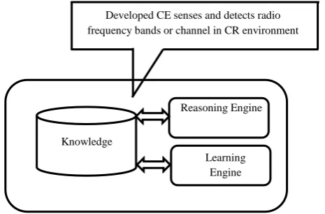
is an integer 1,2,3,4 … while Nis the points of fast Fourier transform. Equation (2) was used in determining the time taken in detecting primary radio signals in a cognitive radio environment. The ideal sensing time parameters obtained from (2) were used in the third stage to ensure that the cooperative spectrum sensing can work effectively without incurring a cooperative overhead. Interested reader(s) can read our early papers [16,20] for details information on these two stages.The third stage was centered on the development of proposed GUI spectrum sensing algorithm, which its architecture is shown in Figure 2. The GUI spectrum sensing algorithm or CE is called SSADA. SSADA is an acronym for Spectrum Sensing and Detection Algorithm. It is a software algorithm developed to demonstrate spectrum sensing procedures, as well as series of measures to ensure optimal cooperative gain without incurring cooperative overhead. SSADA was written using the Java programming language.
Figure 2. Developed GUI Spectrum Sensing Architecture.
Learning Engine Reasoning Engine Developed CE senses and detects radio frequency bands or channel in CR environment
Knowledge
SSADA consists of three components, namely a knowledge base, a learning engine and a reasoning engine, as shown in Figure 2. It was developed in such a way that it can learn and store lessons as experience in the knowledge base. This experience can be retrieved to perform similar actions and decisions when needed in the future. Based on past experiences and interactions with information in both the learning engine and the reasoning engine, the knowledge base generates the final decision for the SSADA.
The reasoning engine in this study serves as action repository system for the SSADA. The actions stored in the reasoning engine are precondition actions defining the operations the reasoning engine should perform based on the status of the PU activities. The precondition action the reasoning engine performs is to infer either an idle or occupied spectrum band. The reasoning engine therefore looks at the current status of the spectrum to determine the right actions ideal for that condition. Based on the precondition action taken, the knowledge base evaluates the appropriateness of the reasoning engine action based on its past experience.
The learning engine in this study is the ADAMR classifier developed in the first stage using an artificial neural network (ANN). Its major function is to precisely characterize a primary user’s activities by monitoring the modulation scheme on the radio channel in an effort to find a means of optimizing radio spectrum utilization. The first role of the learning engine in this study is to provide radio frequency band statistics of “1” and “0”, each denoting an occupied channel or an idle channel respectively. This is intended to predict the probability of secondary frequency usage. Its second function is to update both the knowledge base and the reasoning engine with its experience on the channel per time period. As the learning engine learns about different radio frequency bands or channels, it will store these lessons in the knowledge base for future use by the reasoning engine.
The sequential functionality and other activities involved in the development of SSADA are illustrated in Figure 3. The overall operation of the GUI spectrum sensing algorithm or SSADA is initiated in stage 1 of Figure 3, by choosing a wireless service of interest in the developed graphic user interface program. A hypothetical South Africa frequency allocation table was used for the spectrum sensing and detection demonstration activities using four wireless services’ frequency bands namely radio broadcasting, television broadcasting, mobile telephone and unlicensed, or ISM frequency bands. The four frequency bands were stored in the knowledge base in Figure 2, which serves as the database for the developed SSADA. In addition, the latitude and longitude of the six main cities in South Africa, namely Bloemfontein, Cape Town, Durban, Johannesburg, Port Elizabeth and Pretoria, used as the test sites, were stored in the database to provide information about the location of each of the cities. After providing the preference service and location, the reasoning engine in Figure 2 was updated with this data and the developed SSADA commences rough spectrum sensing by scanning over the entire system bandwidth (BSYS).
Vol. 2, No. 2, 2015
Figure 3. Developed GUI Flowchart.
START
Start Spectrum Sensing
Enter Preference Service and Location
Start rough sensing by scanning BSYS
Is any modulation scheme detected?
Yes No
Note the channel as idle
Record the channel status as 0
Calculate TRRS value and store
Go to the next channel
Note the channel as occupied
Record the channel status as 1
Go to the next channel
STAGE 2
Is any modulation scheme detected?
Yes No
Update the channel status as0
Calculate TFRS value and store
Report channel status to MN
Go to the next channel
STAGE 3
Start fine sensing by scanning BBLK
Note the channel as occupied
Update the channel status as 1
Report channel status to MN
Go to the next channel Note the channel as idle
STAGE 1
Is logic output 1?
Yes No
Confirm channel as idle
Update the channel status safe
CR or SU can transmit.
Start Spectrum Sensing
Confirm channel as occupied
Update channel status unsafe
Start Spectrum Sensing
STAGE 4
MN transmits “OR” logic result to CR or SU
Calculation of total spectrum sensing time or duration (TS)
MN combines observations from STAGE 3
MN makes final decision on observations using “OR” logic
Table 1. Table of FM Broadcasting Frequency Bands
System Bandwidth (BSYS)/MHz Band Allocation
87.00 87.23 87.46 87.69 87.92 88.15 88.40 Band 1
88.50 88.73 88.96 89.19 89.42 89.65 89.90 Band 2
90.00 90.23 90.46 90.69 90.92 91.15 91.40 Band 3
91.50 91.73 91.96 92.19 92.42 92.65 92.90 Band 4
93.00 93.23 93.46 93.69 93.92 94.15 94.40 Band 5
94.50 94.73 94.96 95.19 95.42 95.65 95.90 Band 6
96.00 96. 23 96.46 96.69 96.92 97.15 97.40 Band 7
97.50 97.73 97.96 98.19 98.42 98.65 98.90 Band 8
99.00 99.23 99.46 99.69 99.92 100.15 100.40 Band 9
100.50 100.73 100.96 101.19 101.42 101.65 101.90 Band 10
102.00 102.23 102.46 102.69 102.92 103.15 103.40 Band 11
103.50 103.73 103.96 104.19 104.42 104.65 104.90 Band 12
105.00 105.23 105.46 105.69 105.92 106.15 106.40 Band 13
106.50 106.73 106.96 107.19 107.42 107.65 107.90 Band 14
108.00 108.23 108.46 108.69 108.92 109.15 109.40 Band 15
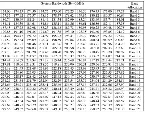
Table 2. Table of Television Broadcasting Frequency Bands
System Bandwidth (BSYS)/MHz Band
Allocation
174.00 174.25 174.50 174.75 175.00 176.25 176.50 176.75 177.00 177.27 Band 1
177.37 177.62 177.37 178.12 178.37 179.62 179.87 180.12 180.37 180.64 Band 2
180.74 180.99 181.24 181.49 181.74 182.99 183.24 183.49 183.74 184.01 Band 3
184.11 184.36 184.61 184.86 185.11 186.36 186.61 186.86 187.11 187.38 Band 4
187.48 187.73 187.98 188.23 188.48 189.73 189.98 190.23 190.48 190.75 Band 5
190.85 191.10 191.35 191.60 191.85 193.10 193.35 193.60 193.85 194.12 Band 6
194.22 194.47 194.72 194.97 195.22 196.47 196.72 196.97 197.22 197.49 Band 7
197.59 197.84 198.09 198.34 198.59 199.84 200.09 200.34 200.59 200.86 Band 8
200.96 201.21 201.46 201.71 201.96 203.21 203.46 203.71 203.96 204.23 Band 9
204.33 204.58 204.83 205.08 205.33 206.58 206.83 207.08 207.33 207.60 Band 10
207.70 207.95 208.20 208.45 208.70 209.95 210.20 210.45 210.70 210.97 Band 11
211.07 211.32 211.57 211.82 212.07 213.32 213.57 213.82 214.07 214.34 Band 12
214.44 214.69 214.94 215.19 215.44 216.69 216.94 217.19 217.44 217.71 Band 13
217.81 218.06 218.31 218.56 218.81 220.06 220.31 220.56 220.81 221.08 Band 14
221.18 221.43 221.68 221.93 222.18 223.43 223.68 223.93 224.18 224.45 Band 15
224.55 224.80 225.05 225.30 225.55 226.80 227.05 227.30 227.55 227.82 Band 16
227.92 228.17 228.42 228.67 228.92 230.17 230.42 230.67 230.92 231.19 Band 17
231.29 231.54 231.79 232.04 232.29 233.54 233.79 234.04 234.29 234.56 Band 18
234.66 234.91 235.16 235.41 235.66 236.91 237.16 237.41 237.66 237.90 Band 19
238.00 238.61 239.22 239.83 240.44 243.49 244.10 244.71 245.32 245.90 Band 20
246.00 246.06 246.12 246.18 246.24 246.54 246.60 246.66 246.72 246.79 Band 21
246.89 246.95 247.01 247.07 247.13 247.43 247.49 247.55 247.61 247.68 Band 22
247.78 247.84 247.90 247.96 248.02 248.32 248.38 248.44 248.50 248.57 Band 23
248.67 248.73 248.79 248.85 248.91 249.21 249.27 249.33 249.39 249.46 Band 24
Vol. 2, No. 2, 2015
Table 3. Table of Mobile Phone Frequency Bands
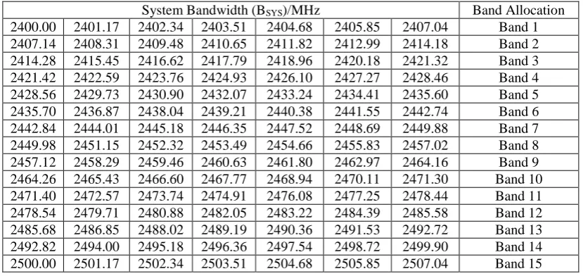
Table 4. Table of Industrial, Scientific and Medical (ISM) Frequency Bands
System Bandwidth (BSYS)/MHz Band Allocation
2400.00 2401.17 2402.34 2403.51 2404.68 2405.85 2407.04 Band 1 2407.14 2408.31 2409.48 2410.65 2411.82 2412.99 2414.18 Band 2 2414.28 2415.45 2416.62 2417.79 2418.96 2420.18 2421.32 Band 3 2421.42 2422.59 2423.76 2424.93 2426.10 2427.27 2428.46 Band 4 2428.56 2429.73 2430.90 2432.07 2433.24 2434.41 2435.60 Band 5 2435.70 2436.87 2438.04 2439.21 2440.38 2441.55 2442.74 Band 6 2442.84 2444.01 2445.18 2446.35 2447.52 2448.69 2449.88 Band 7 2449.98 2451.15 2452.32 2453.49 2454.66 2455.83 2457.02 Band 8 2457.12 2458.29 2459.46 2460.63 2461.80 2462.97 2464.16 Band 9 2464.26 2465.43 2466.60 2467.77 2468.94 2470.11 2471.30 Band 10 2471.40 2472.57 2473.74 2474.91 2476.08 2477.25 2478.44 Band 11 2478.54 2479.71 2480.88 2482.05 2483.22 2484.39 2485.58 Band 12 2485.68 2486.85 2488.02 2489.19 2490.36 2491.53 2492.72 Band 13 2492.82 2494.00 2495.18 2496.36 2497.54 2498.72 2499.90 Band 14 2500.00 2501.17 2502.34 2503.51 2504.68 2505.85 2507.04 Band 15
System Bandwidth (BSYS)/MHz Band
Allocation 890.00 890.28 890.56 890.84 891.12 892.52 892.80 893.08 893.36 893.58 Band 1 893.68 893.96 894.24 894.52 894.80 896.20 896.48 896.76 897.04 897.26 Band 2 897.36 897.64 897.92 898.20 898.48 899.88 900.16 900.44 900.72 900.94 Band 3 901.04 901.32 901.60 901.88 902.16 903.56 903.84 904.12 904.40 904.62 Band 4 904.72 905.00 905.28 905.56 905.84 907.24 907.52 907.80 908.08 908.30 Band 5 908.40 908.68 908.96 909.24 909.52 910.92 911.20 911.48 911.76 911.98 Band 6 912.08 912.36 912.64 912.92 913.20 914.60 914.88 915.16 915.44 915.66 Band 7 915.76 916.04 916.32 916.60 916.88 918.28 918.56 918.84 919.12 919.34 Band 8 919.44 919.72 920.00 920.28 920.56 921.96 922.24 922.52 922.80 923.02 Band 9 923.12 923.40 923.68 923.96 924.24 925.64 925.92 926.20 926.48 926.70 Band 10 926.80 927.08 927.36 927.64 927.92 929.32 929.60 929.88 930.16 930.38 Band 11 930.48 930.76 931.04 931.32 931.60 933.00 933.28 933.56 933.84 934.06 Band 12 934.16 934.44 934.72 935.00 935.28 936.68 936.96 937.24 937.52 937.74 Band 13 937.84 938.12 938.40 938.68 938.96 940.36 940.64 940.92 941.20 941.42 Band 14 941.52 941.80 942.08 942.36 942.64 944.04 944.32 944.60 944.88 945.10 Band 15 945.20 945.48 945.76 946.04 946.32 947.72 948.00 948.28 948.56 948.78 Band 16 948.88 949.16 949.44 949.72 950.00 951.40 951.68 951.96 952.24 952.46 Band 17 952.56 952.84 953.12 953.40 953.68 955.08 955.36 955.64 955.92 956.14 Band 18 956.24 956.52 956.80 957.08 957.36 958.76 959.04 959.32 959.60 959.90 Band 19 960.00 1028.45 1096.90 1165.35 1233.80 1576.05 1712.95 1644.50 1781.40 1849.90 Band 20 1850.00 1851.19 1852.38 1853.57 1854.76 1860.71 1861.90 1863.09 1864.28 1865.46 Band 21
To ascertain the particular modulation detected by the algorithm, the developed ADAMR was designed in a matrix form called a table of Modulation Scheme Detection Matrix (MSDM), as shown in Figure 4. The position of “1”, in each row of the table indicates the presence of the corresponding modulation scheme in the channel. This table of MSDM, Figure 4, is used in stages 2 and 3 in Figure 3 to detect the presence of the modulation scheme in the channel.
NONE QAM QAM OFDM FM SSB DSB AM QPSK BPSK FSK ASK ASK MSDM 64 16 2 4 2 0 0 0 0 0 0 0 0 0 0 0 0 1 0 0 0 0 0 0 0 0 0 0 0 1 0 0 0 0 0 0 0 0 0 0 0 1 0 0 0 0 0 0 0 0 0 0 0 1 0 0 0 0 0 0 0 0 0 0 0 1 0 0 0 0 0 0 0 0 0 0 0 1 0 0 0 0 0 0 0 0 0 0 0 1 0 0 0 0 0 0 0 0 0 0 0 1 0 0 0 0 0 0 0 0 0 0 0 1 0 0 0 0 0 0 0 0 0 0 0 1 0 0 0 0 0 0 0 0 0 0 0 1 0 0 0 0 0 0 0 0 0 0 0 1 0 0 0 0 0 0 0 0 0 0 0 1 0 0 0 0 0 0 0 0 0 0 0 0
Figure 4. Modulation Scheme Detection Matrix .
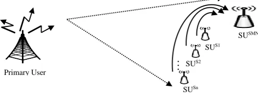
In stage 3, a fine spectrum-sensing operation is executed. If any of the modulation schemes are detected, the channel is noted as occupied and finally the status of the channel during this local sensing process is updated as “1”, in the learning engine. However, if there is no modulation scheme in the channel, the channel is noted as idle and its status is updated as “0”, in the learning engine. These binary observations of “1” and “0”, for occupied and idle channels respectively, are the results of the local spectrum sensing that are reported to the secondary user master mode sensor (SUSMN) by
secondary user sensors (SUSs). This local sensing reporting procedure is illustrated in Figure 5. Also,
at this stage, the time taken to carry out the total spectrum sensing (TFRS) is calculated using (2). The
calculated TFRS value is stored in the learning engine.
Figure 5. Local Cooperative Sensing Reporting Model.
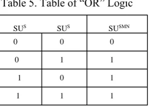
In stage 4, depicted in Figure 3, which is the last stage of the algorithm, terminates one complete cycle. In the stage, the SUSMN combines all the binary observations from the third stage
using “OR” logic, as illustrated in Table 5. The “OR” logic was used to prevent both false and miss detection rate probabilities. Furthermore, in this stage, the “OR” logic result is tested. If the “OR” logic result is “1”, the channel is confirmed as occupied and unsafe for secondary transmission by SU.
Vol. 2, No. 2, 2015
However, if the “OR” logic result testing is “0”, the channel is confirmed as idle and safe for secondary or opportunistic usage. The result of the “OR” logic test provides the final decision on the channel. When the final decision is made like this, the SUSMN, also known as MN, transmits the final
decision for opportunistic secondary transmission possibility to the CR or SU as illustrated in Figure 5. The algorithm finally determines the total time (TS) taken to carry out the overall spectrum-sensing
using (2). After a complete cycle like this, the spectrum sensing by the SUS starts all over again while
SU is transmitting on the detected idle channel.
Table 5. Table of “OR” Logic
The SSADA working environment is shown in Figure 6. It consists of three modules and is capable of performing three basic functions. The first module is the preferred service and location, which enables SSADA to scan the overall preferred service allocated frequency band in South Africa. The location included enables SSADA to decide upon an appropriate idle channel to claim opportunistically using DSA so as not to cause co-channel interference to a primary user resulting from a re-used frequency.
The second module on an SSADA working environment is the plotting section, where the sensing time parameters selection for optimizing cooperative spectrum sensing gain can be derived. The third module in an SSADA working environment is the manual calculations section, for determining sensing time (Ts). The basic different between this third module and the second module is that it presents its results in numerals, while the second module presents its results in a graphical form. The evaluation of the developed SSADA or GUI, described above, in achieving the desired objective of the study is presented in the next section.
Figure 6. The developed GUI Attributes.
0 0
0
0
0 1
1
1
1
1
1
4. Performance Evaluation of the developed GUI
This section showcases some of the capabilities of the developed GUI or SSADA. The three modules on GUI are demonstrated using the four wireless services employed. Detailed activities of each module are showcased with typical examples in the following two sub-sections.
4.1. SSADA Spectrum Scanning Module Application
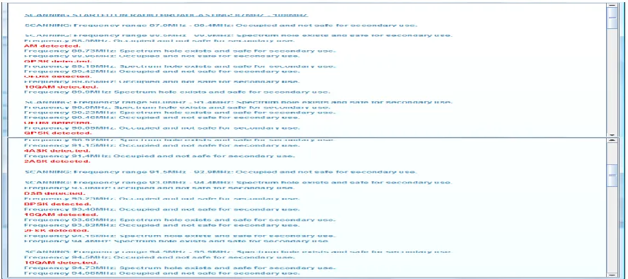
This subsection presents the application of the first module of GUI. In using the module, the user needs to choose the preferred service. The preferred service is chosen by selecting either the block or the drop down arrow () beside it. This will bring down a dialog box that contains the four services, namely radio broadcasting, television broadcasting, mobile telephone and ISM. The user then selects the preferred one. The user can subsequently run the program by selecting ‘run-block’. Selecting this option activates the program to carry out overall spectrum sensing or scanning for the selected or preferred wireless service. A typical result of such an overall radio broadcasting system scanning exercise is shown in Figure 7.
Figure 7. Typical GUI Spectrum Sensing Result for Radio Broadcasting.
Vol. 2, No. 2, 2015
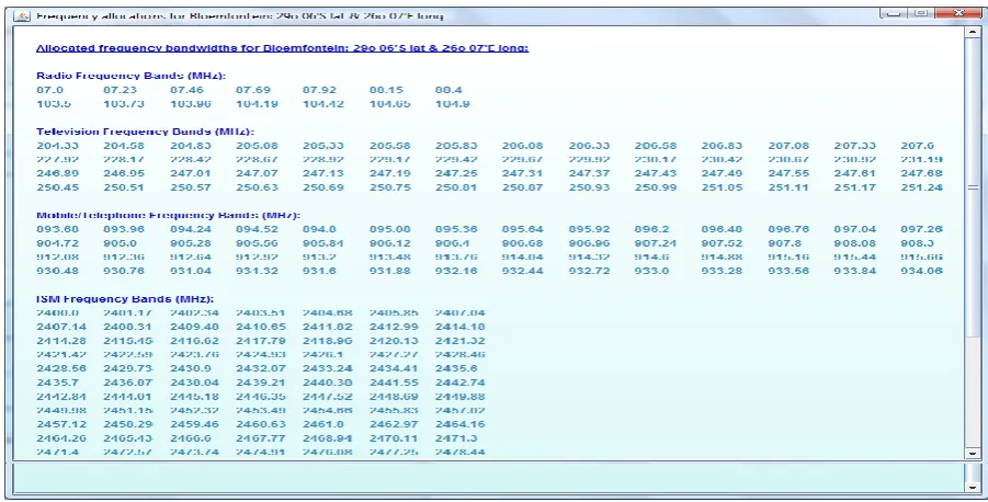
Figure 8. GUI Overall Table of Frequency Allocation for Bloemfontein.
4.2. GUI Sensing Time (Ts) Plots Module Application
This subsection is devoted to demonstration of the second module of the developed GUI or SSADA. The module was developed to generate four different plots for determining ideal sensing time parameters settings for optimal cooperative gain, without incurring a cooperative overhead. In this module, the user needs to first select the type of service parameter to use its table of allocation. The second step is to select the type of plot to be generated by selecting either the plot block or the drop down arrow () beside it and a dialog box that contains the four plots, namely variation of Ts with M, variation of Ts with FRES, variation of Ts with M at different values of alpha (α) and the variation of Ts
with N, will drop down for the user to select the preferred plot type. The next step is to input the values of α, the FFT size (N) and the fine resolution frequency (FRES). The user does not need to input
the system’s bandwidth (BSYS) value because the GUI plot’s module takes the value directly from the
table of frequency allocation. Typical performance results obtained are presented as follows.
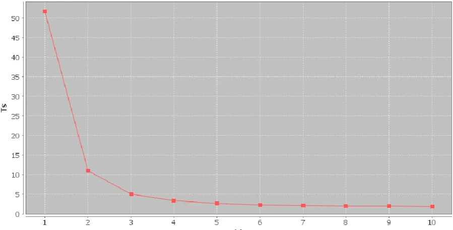
4.2.1. Sensing Time (Ts) Plot against Number of Cognitive Radio (M)
Figure 9. GUI Generated Ts Plot against Number of Cognitive Radio (M).
From Figure 9, it is observed that the sensing time (TS) decreases with increasing number of
cognitive radios. However, as the number of cognitive radios collaborating becomes four, a point of diminishing returns is reached. Hence, after M = 4, an increase in the number of cognitive radios is not justified given the small decrease in sensing time achieved. Based on this observation, this research work established that a maximum of four cognitive radios users are ideal for optimal cooperation gain in a cognitive radio environment in order to avoid incurring cooperative overhead.
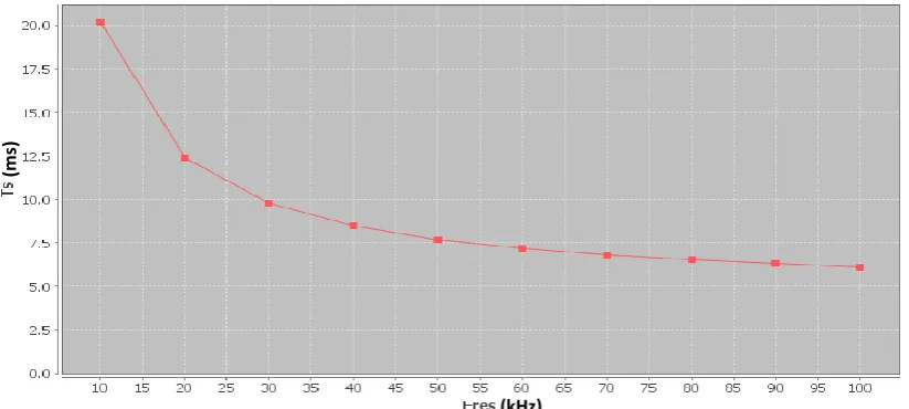
4.2.2. Sensing Time (Ts) Plot against FRES
This second GUI plotting module application follows the same step described in sub-section 4.2.1. In demonstrating this plot, the mobile phone parameters for Johannesburg were used. The system bandwidth (BSYS) was automatically selected by the GUI with constant values of α = 10 and N
= 32 while FRES was varied from 10 kHz to 100 kHz. The result obtained is shown in Figure 10. Like
the number of cognitive radios, FRES is inversely proportional to the sensing time, TS. Hence, a
theoretical assumption that a high value of FRES will improve the cooperative gain without incurring
Vol. 2, No. 2, 2015
Figure 10. GUI or SSADA Generated Ts Plot against FRES.
From Figure 10, it is it is observed that the TS decreases with increase in fine frequency sensing
resolution until 60 kHz, when a point of diminishing returns is reached. Hence, after this frequency, observations show that an increase in fine frequency sensing resolution does not justify the small decrease in sensing time. This shows that for optimal cooperation gain, an appropriate fine frequency sensing resolution needs to be determined, so as not to incur a cooperative overhead.
4.2.3. Sensing Time (Ts) Plot against M at different Values of α
This GUI or SSADA module application also follows the same steps described in sub-section 4.2.1. In demonstrating this plot, the TV broadcasting parameters were used with Durban as the preferred location or test site. The BSYS was automatically selected by the GUI. The values of M were
varied from 2 to 4, while the values of alpha (α) were also varied from 10 to 50 with constant values of N = 32 and FRES = 10 Hz respectively. The plot obtained is shown in Figure 11.
Figure 11. GUI Generated Ts Plot against M at different values of α.
(ms)
Considering Figure 11, which shows the plot of sensing time against the number of cognitive radios at different values of α, it is noted that for a small number of cognitive radios, for example M = 2, a large value of α gives a minimal sensing time and vice-versa. However, this is not generally true as the number of cognitive radios collaborating for spectrum sensing increase. For instance, when the four cognitive radios collaborate for spectrum sensing were considered, the numerical result obtained from the algorithm shows that minimum sensing time was obtained at α = 30, rather than at α = 50. This shows that, as values of α increase beyond a certain point, it is only adding to the number of blocks to be scanned during the fine sensing process, rather than contributing to a fast sensing rate. Hence, in a practical implementation of cooperative sensing, the appropriate value of α needs to be wisely selected in order to achieve optimal cooperative gain without incurring a cooperative overhead. Based on the fixed parameters used, as well as four maximum numbers of cooperative sensors or cognitive radios suggested for collaborative sensing in this study, the ideal value of α for optimal cooperative gain without incurring a cooperative overhead is 30.
4.2.4. Sensing Time (Ts) Plot against FFT size (N)
This GUI module demonstration was carried out using the radio broadcasting frequency table. Pretoria was chosen as the preferred location or test site. The BSYS was automatically selected by the
GUI. The values of N were varied from 16 to 1024 with constant values of M = 4, α = 10 and FRES =
10 Hz respectively. The plot obtained is shown in Figure 12.
Figure 12. GUI Generated Ts Plot against FFT size (N).
4.3. SSADA Plot Module Editing Environment
In GUI plot module, copying of the plots can be done in two ways. The first is by following the process for the first module whereby the ‘Ctrl + Alt + Print Scrn’ keys are pressed together to copy the screen and paste the plots on Microsoft Word. The second approach is by right-clicking the mouse on the plot environment to bring down the inbuilt editing feature incorporated in this second module, as shown in Figure 13. Apart from copying the plot, other editing can be done on the plots as shown in Figure 13 by right click on the graph.
Vol. 2, No. 2, 2015
Figure 13. In-built Editing Capability for the GUI Plot Module.
4.4. The GUI Manual Calculation
The manual calculation module is the third working module on the developed GUI working environment. Unlike the two other modules, the BSYS value is not automatically selected. The user has
to input all the required values on the keyboard for the GUI manual calculations’ module to work. Copying of the manual calculations’ module result follows the same procedure as the first module, whereby the ‘Ctrl + Alt + Print Scrn’ keys are pressed together to copy the screen and paste the results on Microsoft Word using the paste command. A typical example of its usage is presented in Figure 14 using the ISM parameter in Table 4.
Figure 14. The GUI Typical Manual Calculation Demonstration.
5. Conclusion
In this paper, a GUI sensing algorithm called SSADA was developed and evaluated. The evaluation results of the algorithm using the four wireless services shows that the developed algorithm performs favorably well. In addition, the capability of the developed SSADA that could scan all the hypothetical allocated frequency bands for the four wireless services within the country is an indication that the developed GUI sensing algorithm can enhance OSA or DSA deployment in any part of the country. Similarly, since the hypothetical allocated frequency bands can be replaced by any frequency bands of any country, makes the developed GUI sensing algorithm deployment applicable to any part of the world. In addition, the performance evaluation results on the developed GUI spectrum sensing algorithm for this study have shown that not only does the detection method perform well, but that the overall objective of the study has been achieved.
Acknowledgements
The authors thank all the sponsors of the University of the Witwatersrand’s Centre for Telecommunications Access and Services (CeTAS) for their financial support. The authors also express their appreciation to the Independent Communications of South Africa (ICASA) for its financial support. The principal author also acknowledges the financial assistance received from the University of the Witwatersrand’s Postgraduate Merit Award (PMA).
References
[1] Cave, M., Foster, A. and Jones, R. W. (2006). Radio Spectrum Management: Overview and Trends, Proc. of ITU Spectrum Workshop 2006, pp. 1–22, September 2006, Online [Available]:
http://www.itu.int/osg/spu/stn/spectrum/workshop_proceedings/Background_Papers_Final/Adrian%20Fost
er%20-%20CONCEPT_PAPER_20_9_06_Final.pdf. Accessed on 4 November 2008.
[2] Nunno, R. M. (2002). Review of Spectrum Management Practices. Fed. Comm. Commission Int. Bureau Strategic Analysis and Negotiations Division, pp. 1–15. Online [Available]:
http://www.ictregulationtoolkit.org/en/Document.2270.pdf. Accessed on 16 August 2008.
[3] Olafsson, S., Glover, B. and Nekovee, M. (2007). Future Management of Spectrum. BT Technology Journal, Vol. 25, No. 2, pp. 52–63.
[4] Akyildiz, I. F., Lee, W. Y., Vuran, M. C. and Mohanty, S. (2007). Next Generation/Dynamic Spectrum Access/Cognitive Radio Wireless Networks: A Survey. Computer Networks Journal, Vol. 50, No. 13, pp. 2127–2159.
[5] Haykin, S. (2005). Cognitive Radio: Brain-Empowered wireless Communications. IEEE Journal on Selected Areas in Communications,Vol. 23, No. 2, pp. 201–220.
[6] Scutari, G., Palomar, D. P., and Barbarossa, S. (2008). Cognitive MIMO Radio Competitive Optimality Design Based on Subspace Projections. IEEE Signal Processing Magazine, pp. 46–59.
[7] FCC (2002). Spectrum Policy Task Force Report. FCC Document ET Docket No. 02-135, pp.1–22. Online [Available]: http://transition.fcc.gov/sptf/files/E&UWGFinalReport.pdf. Accessed on 19 May 2008. [8] Song, Y. Fang, Y., and Zhang, Y. (2007), Stochastic Channel Selection in Cognitive Radio Networks. In
IEEE Proc. of Global Communications Conference (GLOBECOM), Washington, DC, pp. 4878–4882. [9] Chen, R., Park, J-M., and Reed, J. H. (2008). Defense against Primary User Emulation Attacks in Cognitive
Radio Networks. IEEE Journal on Selected Areas in Communications, Vol. 26, No. 1, pp. 25–37.
[10] Čabrić, D., Mishra, S. M., Willkomm, D., Brodersen, R., and Wolisz, A. (2005). A Cognitive Radio Approach for Usage of Virtual Unlicensed Spectrum. InProc. of 14th 1st Mobile Wireless Communications
Summit. Online [Available]: http://www.eurasip.org/Proceedings/Ext/IST05/papers/411.pdf. Accessed on 26 January 2015.
Vol. 2, No. 2, 2015
[12] Čabrić, D., and Brodersen, R. W. (2005). Physical Layer Design Issues Unique To Cognitive Radio Systems. InProceedings of 16th IEEE International Symposium on Personal, Indoor and Mobile Radio Communications (PIMRC 2005), Berlin, 759–763.
[13] Čabrić, D., Tkachenko, A., and Brodersen, R. W. (2006). Spectrum Sensing Measurements of Pilot, Energy, and Collaborative Detection. InProc. of IEEE Military Communications Conference (MILCOM), Washington, DC, USA, pp. 1–7.
[14] Gandetto, M., and Regazzoni, C. (2007). Spectrum Sensing: A Distributed Approach for Cognitive Terminals. IEEE Journal on Selected Areas in Communications, Vol. 25, No. 3, pp. 546–557.
[15] Larsson, E. G., and Regnoli, G. (2007). Primary System Detection for Cognitive Radio: Does Small-Scale Fading Help? IEEE Communication Letters, Vol. 11, No. 10, pp. 799–801.
[16] Popoola, J. J., and van Olst, R. (2011). Cooperative Sensing Reliability Improvement for Primary Radio Signal Detection in Cognitive Radio Environment. In Proc. of Southern Africa Telecommunication Networks and Applications Conf. (SATNAC), East London, South Africa, pp. 131– 136.
[17] Lee, C.-H., and Wolf, W. (2008). Energy Efficient Techniques for Cooperative Spectrum Sensing in Cognitive Radios. In Proc. of 5th IEEE Consumer Communications and Networking Conference (CCNC), Las Vegas, NV, pp. 968–972.
[18] Akyildiz, I. F., Lo, B. F., and Balakrishnan, R. (2011). Cooperative Spectrum Sensing in Cognitive Radio Networks: A Survey. Physical Communication. Vol. 4, No. 1, pp. 40–62.
[19] Mishra, S. M., Sahai, A., and Brodersen, R. (2006). Cooperative Sensing among Cognitive Radios. In Proc. of IEEE Inter. Conf. on Communications (ICC), Istanbul, pp. 1658–1663.
[20] Popoola, J. J., and van Olst, R. (2013). The Performance Evaluation of a Spectrum Sensing Implementation using an Automatic Modulation Classification detection Method with a Universal Software Radio Peripheral. An International Journal on Expert Systems with Applications, Vol. 40, No. 6, pp. 2165– 2173.
Authors
Jide Julius Popoola
Jide Julius Popoola received B.Eng.[Hons] and M.Eng.[Communications] degrees from the Federal University of Technology, Akure, Nigeria. He obtained his PhD degree from University of the Witwatersrand, Johannesburg, South Africa under the supervision of Prof. Rex van Olst. His research interests include wireless communications and signal processing with a focus on cognitive radios, spectrum management and dynamic spectrum allocation. He has several publications in both local and international Journals and Conferences. He lectures in the Department of Electrical and Electronics Engineering, Federal University of Technology, Akure, Nigeria
Rex van Olst
![Figure 1. Spectrum Utilization Profile [4].](https://thumb-us.123doks.com/thumbv2/123dok_us/8774819.1758913/3.595.90.468.94.251/figure-spectrum-utilization-profile.webp)