Two Faces of the Framework for Analysis and Prediction, Part 1 - Education

(1)

249

Information Technology and Control 2018/2/47

Two Faces of the Framework

for Analysis and Prediction,

Part 1 - Education

ITC 2/47

Journal of Information Technology and Control

Vol. 47 / No. 2 / 2018 pp. 249-261

DOI 10.5755/j01.itc.47.2.18746 © Kaunas University of Technology

Two Faces of the Framework for Analysis and Prediction, Part 1 - Education

Received 2017/08/02 Accepted after revision 2018/03/07

http://dx.doi.org/10.5755/j01.itc.47.2.18746

Corresponding author: [email protected]

Vladimir Kurbalija, Mirjana Ivanović

Department of Mathematics and Informatics, Faculty of Sciences, University of Novi Sad, Trg D. Obradovića 4, 21000 Novi Sad, Serbia, {kurba,mira}@dmi.uns.ac.rs

Zoltan Geler

Department of Media Studies, Faculty of Philosophy, University of Novi Sad, Dr Zorana Đinđića 2, 21000 Novi Sad, Serbia, [email protected]

Miloš Radovanović

Department of Mathematics and Informatics, Faculty of Sciences, University of Novi Sad, Trg D. Obradovića 4, 21000 Novi Sad, Serbia, [email protected]

With the ever-increasing amounts of data being generated in all walks of life and work, data analysis tools are gaining in importance and becoming essential in many application scenarios, including commerce, healthcare, research, and education. One important type of data are time series, which can be viewed as chronologically arranged arrays of numerical values that describe sequences of quantitative observations (e.g. in medical exam-inations, scientific and engineering experiments, etc.). In this article, we survey the successful applications of the Framework for Analysis and Prediction (FAP) – a Java-based tool dedicated to time-series analysis – in the area of education. Its utilization in this domain spans the development of several graphical user interfaces, as well as student projects illustrating and enhancing the capabilities of the system in the domains of time-series reconstruction, medicine (diagnosis), finance (stock value prediction) and psychology.

(2)

Information Technology and Control 2018/2/47 250

1. Introduction

Over the past two decades, due to the increasing need for processing ever-growing amounts of data, re-searching different aspects of data mining has gained more and more attention, becoming an important part of computer science and education [1]. Data min-ing can be described as the process of revealmin-ing and extracting potentially useful knowledge, interesting information, and novel patterns from vast quantities of data in order to support a wide range of decision making processes [12]. To accomplish this task, it combines solutions from several related research ar-eas, such as machine learning, statistics, and database systems [29].

Temporal data mining is a sub-field of data mining that is focused on knowledge discovery from large collections of temporal data [25]. This form of data represents time-ordered sequences of numerical or categorical values. The most common type of tem-poral data are time series: they are composed of real values usually sampled at regular time intervals [11]. Such chronologically arranged arrays of numbers are used to express the change of the observed phenom-ena over time in a broad spectrum of different areas including finance, economics, medicine, engineering, meteorology, oceanography as well as in many other fields of natural and social sciences [2].

Statistical analysis of time series has a long histo-ry [15] and its main objectives are identifying pat-terns, trend analysis, seasonality and forecasting [4]. However, time-series data mining is concerned with tasks like indexing, classification, clustering, prediction, anomaly detection, data representation, and distance measures [7, 27]. According to Laxman and Sastry [22], there are some significant differenc-es between statistical analysis and temporal data mining: data-mining applications must effectively analyze much larger volumes of data and their field of interest exceeds the scope of statistical time-se-ries analysis.

The possibility of applying time series for storage, analysis, and visualization of data collected in many diverse domains led to a significant growth of inter-est in researching different task types of time-series data mining and resulted in a large amount of papers

introducing new techniques and algorithms. How-ever, alternative solutions are usually sporadically introduced in different publications and separately implemented, making it difficult to reproduce the presented results. Moreover, the newly-introduced methods have always claimed a particular superiority over some of the previous ones [27].

Taking these considerations into account, it is clear that the availability of a free and open sourced li-brary could support and facilitate researching new and comparing existing techniques in this domain. Furthermore, it could be used as an auxiliary tool in research and education. Motivated by these delib-erations, we have developed an extensible software package that implements many of the most import-ant algorithms in the field of time-series data min-ing. Our framework facilitates numerous activities and applications of time series, including distance/ similarity measures, preprocessing, classification, and time-series representations. The basic concepts of our Framework for Analysis and Prediction (FAP) were presented in [20]. In this paper, we will give a detailed overview of the capabilities of FAP, and de-scribe its applications in education realized at our institution, emphasizing the influence each applica-tion has had on the development of FAP. The com-panion paper, Two Faces of FAP, Part 2, will focus on applications in research.

The rest of this paper is organized as follows. Back-ground knowledge on time series and distance mea-sures is presented in the next section. Section 3 de-scribes our Framework for Analysis and Prediction. Section 4 presents applications of the framework in education. Conclusions are given in Section 5.

2. Time Series and Distance

Measures

(3)

engi-251

neering experiments, and they are suitable to charac-terize social, economic, and natural phenomena. Formally, a d-dimensional multivariate time series

Q of length n can be defined as a sequence of ordered pairs Q = (q1, t1), (q2, t2), ..., (qn, tn), where qi∈Rd de-notes the measured value of the observed phenome-non at timestamp ti∈R [1]. In this paper, we consi-der only univariate time series (d = 1) assuming that the measurements were performed at equidistant ti-mestamps (i.e. ti+1 = ti + c, ∀i∈{1, ..., n–1} where c is a constant value). In this manner, the time components of time series can be omitted, thus univariate time se-ries Q can be viewed as a sequence of n real numbers:

Q = (q1, q2, ..., qn) [2].

Since similarity-based retrieval is one of the funda-mental components of many time-series data min-ing tasks, the choice of an (in)appropriate measure is of crucial impact on their outcome [28]. Howev-er, unlike in the case of traditional databases, the similarity/distance1_{between time series cannot be}

determined unambiguously. As a consequence, a great number of different approaches is proposed in the literature [7, 10, 26]. Among them, the two most frequently used time-series distance measures are Euclidean distance and Dynamic Time Warping (DTW) [9].

Euclidean distance represents a special case of Min-kowski distance which is based on linear aligning of related points of time series: the i-th point of the first

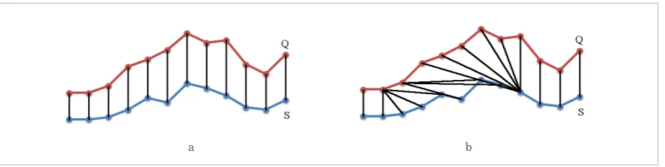
Figure 1

Aligning of time series: (a) linear; (b) non-linear

series is paired with the i-th point of the second one (Fig. 1a). Let Q = (q1, q2, ..., qn) and S = (s1, s2, ..., sm) denote two univariate time series of the same length (n = m). Then, Euclidean distance is calculated as follows:

Taking these considerations into account, it is clear that the availability of a free and open sourced library could support and facilitate researching new and comparing existing techniques in this domain. Furthermore, it could be used as an auxiliary tool in research and education. Motivated by these deliberations, we have developed an extensible software package that implements many of the most important algorithms in the field of time-series data mining. Our framework facilitates numerous activities and applications of time series, including distance/similarity measures, preprocessing, classification, and time-series representations. The basic concepts of our Framework for Analysis and Prediction (FAP) were presented in [20]. In this paper, we will give a detailed overview of the capabilities of FAP, and describe its applications in education realized at our institution, emphasizing the influence each application has had on the development of FAP. The companion paper, Two Faces of FAP, Part 2, will focus on applications in research.

The rest of this paper is organized as follows. Background knowledge on time series and distance measures is presented in the next section. Section 3 describes our Framework for Analysis and Prediction. Section 4 presents applications of the framework in education. Conclusions are given in Section 5. 2. Time Series and Distance Measures

A time series is a chronologically arranged array of numerical values that describes a sequence of quantitative observations [15]. Time series can represent results of medical examinations, scientific and engineering experiments, and they are suitable to characterize social, economic, and natural phenomena. Formally, a d-dimensional multivariate time series Q of length n can be defined as a sequence of ordered pairs � 𝑑 ��𝑞𝑞�, 𝑡𝑡��, �𝑞𝑞�, 𝑡𝑡��, … , �𝑞𝑞�, 𝑡𝑡��, where 𝑞𝑞�∈

𝑅𝑅� _{denotes the measured value of the observed}

phenomenon at timestamp 𝑡𝑡� ϵ 𝑅𝑅 [1]. In this paper, we

consider only univariate time series (𝑑𝑑 𝑑 𝑑) assuming that the measurements were performed at equidistant timestamps (i.e. 𝑡𝑡��𝑑 𝑡𝑡�+ 𝑐𝑐, ∀𝑖𝑖 ∈ �𝑑, … , 𝑛𝑛 𝑛 𝑑�,

where c is a constant value). In this manner, the time

components of time series can be omitted, thus univariate time series Q can be viewed as a sequence of n real numbers: 𝑄𝑄 𝑑 �𝑞𝑞�, 𝑞𝑞�, … , 𝑞𝑞�� [2].

Since similarity-based retrieval is one of the fundamental components of many time-series data mining tasks, the choice of an (in)appropriate measure is of crucial impact on their outcome [28]. However, unlike in the case of traditional databases, the similarity/distance1_{between time series cannot be} determined unambiguously. As a consequence, a great number of different approaches is proposed in the literature [7, 10, 26]. Among them, the two most frequently used time-series distance measures are Euclidean distance and Dynamic Time Warping (DTW) [9].

Euclidean distance represents a special case of Minkowski distance which is based on linear aligning of related points of time series: the i-th point of the first series is paired with the i-th point of the second one (Fig. 1a). Let 𝑄𝑄 𝑑 �𝑞𝑞�, 𝑞𝑞�, … , 𝑞𝑞�� and 𝑆𝑆 𝑑

�𝑠𝑠�, 𝑠𝑠�, … , 𝑠𝑠�� denote two univariate time series of the

same length (𝑛𝑛 𝑑 𝑛𝑛). Then, Euclidean distance is calculated as follows:

𝑑𝑑�𝑄𝑄, 𝑆𝑆� 𝑑 ��𝑞𝑞�𝑛 𝑠𝑠��

��

.

Euclidean distance is a very simple measure and it has many advantages: it is easy to implement, fast to compute and represents a distance metric (allowing it to be used for indexing in time-series databases). However, it has some shortcomings, too: due to the linear aligning of the points, it is sensitive to distortions and shifting along the time axis [14].

To overcome this disadvanta ge, many different elastic distance measures were proposed: Dynamic Time Warping (DTW), Longest Common

1_{unless explicitly stated, we will not distinguish between}

similarity and distance measures, and will use the two terms interchangeably

(a) (b)

Figure 1. Aligning of time series: (a) linear; (b) non-linear

Euclidean distance is a very simple measure and it has many advantages: it is easy to implement, fast to compute and represents a distance metric (allowing it to be used for indexing in time-series databases). However, it has some shortcomings, too: due to the linear aligning of the points, it is sensitive to distor-tions and shifting along the time axis [14].

To overcome this disadvantage, many different elastic distance measures were proposed: Dynam-ic Time Warping (DTW), Longest Common Sub-sequence (LCS), Edit Distance with Real Penalty (ERP), Edit Distance on Real sequence (EDR) [9], Time Warp Edit Distance (TWED) [23] and others. These distance measures rely on non-linear aligning of points – several points of one of the series can be paired with the same point of the other one, as illus-trated in Fig. 1b. In the field of time-series data min-ing, one of the most popular elastic distance mea-sures is DTW [30].

1

1 unless explicitly stated, we will not distinguish between similarity and distance measures, and will use the two terms interchangeably

(4)

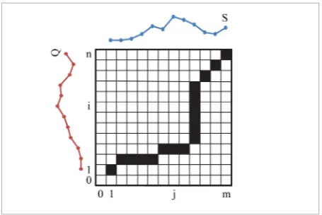
DTW defines the distance between two given time series Q and S of lengths n and m as the minimal ac-cumulated distance between their points. This is achieved by searching for the optimal warping path (Fig. 2) in the warping matrix [Di, j](n+1), m+1.

The optimal warping path which minimizes the warping distance between Q and S can be calculated using dynamic programming based on the following recursive definition:

𝐷𝐷�,�=

⎩ ⎪ ⎨ ⎪

⎧ _∞0 𝑖𝑖 = 𝑗𝑗 = 0,_{𝑖𝑖=0, 𝑗𝑗 >0}_or_{𝑖𝑖 > 0, 𝑗𝑗=0,}

��, 𝑠𝑠�� 𝑖𝑖� �

𝐷𝐷��,��

𝐷𝐷��,�

𝐷𝐷�,��

𝑖𝑖, 𝑗𝑗 ≥ 1,

where d(q_i, s_j) denotes the squared distance between

qi and sj. The distance between Q and S is then defined as DTW(Q, S) = Dn, m.

Figure 2

Optimal warping path inside the warping matrix

𝐷𝐷�𝑖�=

⎩ ⎪ ⎨ ⎪

⎧ _∞0 𝑖𝑖 = 𝑖𝑖 = 0𝑖_{𝑖𝑖 = 0𝑖 𝑖𝑖 𝑖 0𝑖}_or_{𝑖𝑖𝑖 𝑖 0𝑖 𝑖𝑖 = 0𝑖}

��𝑖 𝑠𝑠�� 𝑖𝑖� �

𝐷𝐷��𝑖��

𝐷𝐷��𝑖�

𝐷𝐷�𝑖��

𝑖𝑖𝑖 𝑖𝑖 𝑖 𝑖𝑖

The quadratic computational complexity of finding the distance between time series can make the elastic measures not directly applicable to larger real-world problems. Furthermore, comparing each element of one time series with each element of the other one can lead to pathological aligning of the points (where a relatively small part of one time series maps onto a large section of the other time series). One way to avoid these shortcomings is to constrain the warping path using the Sakoe-Chiba band (Fig. 3a) or the Itak-ura parallelogram (Fig. 3b) [9].

3. Framework for Analysis

and Prediction

Framework for Analysis and Prediction (FAP – http://perun.pmf.uns.ac.rs/fap/) is written in Java and designed to be a free and extensible open-source software package implementing all of the main tech-niques and methods for temporal data mining and analysis. It is developed and maintained at the De-partment of Mathematics and Informatics, Faculty of Sciences, University of Novi Sad, Serbia.

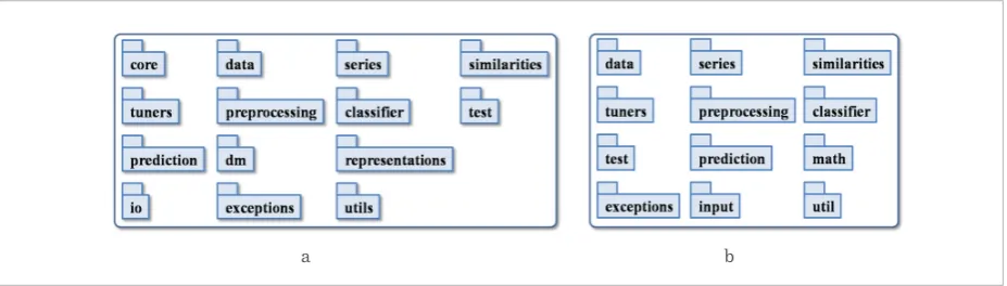
Overall architecture. The overall architecture of the framework is presented in Fig. 4a. The essential part of the library is implemented in the core package (Fig. 4b) which contains basic interfaces and classes that define the fundamental functionality of the sys-tem. In order to comply with the JavaBeans technolo-gy, all of the core classes support object serialization, have a default constructor and public getter and set-ter methods. The concrete implementations of the algorithms are placed in the appropriate subpackages of the library. In the rest of this section, we will sum-marize the fundamental interfaces and classes of the

core package.

Time series. Time series objects are instances of the

TimeSeries class from the fap.core.series package. They are implemented as series of data point objects. Data points are defined by the DataPoint class, and their se-ries are represented by the DataPointSeries class. In addition to the series of data points, every Figure 3

Constraining the warping path using the: (a) Sakoe-Chiba band; (b) Itakura parallelogram

𝐷𝐷�𝑖�=

⎩ ⎪ ⎨ ⎪

⎧ _∞0 𝑖𝑖 = 𝑖𝑖 = 0𝑖_{𝑖𝑖 = 0𝑖 𝑖𝑖 𝑖 0𝑖or𝑖𝑖𝑖 𝑖 0𝑖 𝑖𝑖 = 0𝑖}

��𝑖 𝑠𝑠�� 𝑖𝑖� �

𝐷𝐷��𝑖��

𝐷𝐷��𝑖�

𝐷𝐷�𝑖��

𝑖𝑖𝑖 𝑖𝑖 𝑖 𝑖𝑖

(5)

253

TimeSeries object contains a label (which represents the class of the time series), a supplementary proper-ty called index, and may have several representations. Time-series datasets are realized as objects of type

TimeSeriesArrayList which extends the generic Ar-rayList class and defines several auxiliary methods.

Distance/similarity measures. Similarity measures represent essential ingredients of many time-series data mining tasks. Their role is to describe the sim-ilarity (or dissimsim-ilarity) between time series using numerical values. Classes that represent distance measures need to implement the SimilarityComputor

interface which defines only one method that returns the distance between two given time series (Fig. 5a). FAP contains implementations of several time-series distance/similarity measures, including: Minkows-ki distance (Lp), Euclidean distance (L2), Manhattan

distance (L1), Chebyshev distance (L∞), Canberra tance [5], Kulczynski distance [5], Lorentzian dis-tance [5], Soergel disdis-tance [5], Sørensen disdis-tance [5], Spline distance [19], unconstrained and constrained DTW, LCS, ERP, EDR, and TWED. The constrained ver-sions of the elastic measures are implemented using the Sakoe-Chiba band and the Itakura parallelogram [9].

Preprocessing. Sometimes we need to prepare and clean the raw data before using them, which is achieved by applying different techniques of data preprocessing. Our framework contains implemen-tations of several preprocessing algorithms, includ-ing scalinclud-ing of time-series length, shiftinclud-ing and z-score normalization, min-max normalization, and decimal scaling. Classes that represent preprocessing trans-formations of time series need to implement the Figure 4

Overall architecture: (a) the FAP library; (b) the core package

PreprocessingTransformation interface depicted in Fig. 5b.

Classification. Classification is the process of group-ing objects into predefined categories, classes. It is done on the basis of a selected attribute (class label), which can have a finite number of different values. In this way, we always know the total number of differ-ent classes in advance.

The methods required for implementing classifiers are declared within the Classifier interface (Fig. 5c). The build method conducts training of the classifier based on the given dataset and similarity measure. The classify method is responsible for classifying the given time series. It should return the label selected by the classifying algorithm.

Our library contains the following classifiers: the simple nearest-neighbor classifier (1NN), the major-ity voting k-nearest neighbor classifier (kNN), and the distance-weighted k-nearest neighbor classifi-er in combination with a wide variety of weighting schemes proposed in the literature, like Dudani’s, Ma-cleod’s, the Fibonacci, the uniform and dual-uniform, Zavrel’s, and the dual distance-weighted scheme [9]. The performance of a classifier can be measured by counting the number of correctly and incorrectly classified test objects. The accuracy of a classifier is defined as the ratio of test objects that are correctly classified, and the error rate is defined as the ratio of misclassified test objects. FAP implements the most popular partitioning techniques used to divide the initial set of labeled objects into training and test sets:

holdout, k-fold (stratified) cross-validation, and leave-one-out [12]. In addition, auxiliary classes are

(6)

ed for performing repeated evaluations.

The basic methods for evaluating the performance of classifiers are declared within the Test interface (Fig. 5d). The test method is responsible for carrying out the evaluation process using the given dataset and the classifier set by the setClassifier method. The ge-tErrorRatio method should return the average error ratio. The number of misclassified time series should be returned by the getMisclassified method.

Representations. Storing time series usually re-quires large amounts of space which makes perform-ing different tasks of data minperform-ing more difficult. In addition, sometimes we are not interested in the ex-act values of each time-series data point. For these reasons, time-series databases generally contain only simplified representations of the series. Our library includes several representations, such as the Discrete

Haar Wavelet Transform (Haar), Piecewise Linear

Approximation (PLA), Piecewise Aggregate

Approx-imation (PAA), Symbolic Aggregate Approximation

(SAX) [17], Adaptive Piecewise Constant Approxima-tion (APCA) [13], and Spline [19].

Classes that constitute representations of time series need to implement the TimeSeriesRepresentation

interface which is presented in Fig. 5e. The getValue

method should retrieve the value of the correspond-ing time series at the given value of the time compo-nent. The getOutboundValue method should return the value of time series outside of the range which is covered by current representation.

Resuming and tracking. FAP is designed to enable monitoring of long-time calculations through a call-back mechanism, along with the possibility of their interruption without the loss of already obtained re-sults. The incomplete computations can be resumed later. Tracking the execution of long-running pro-cesses is facilitated through the Callback (Fig. 5f),

CallbackEnabled (Fig. 5g), and Resumable (Fig. 5h) in-terfaces. Combined with object serialization, they en-able storing partial results of time-consuming tasks and the continuation of interrupted operations at a later time.

Methods that are necessary for the implementation of the callback mechanism are defined by the Call-back interface. Classes that provide tracking of their activities should implement the CallbackEnabled in-terface and should regularly call the callback method

of the appropriate Callback object in accordance with the configuration set through the

getDesiredCallback-Number and setPossibleCallbackNumber methods.

The first of these two methods indicates how many times it is expected that they call the callback meth-od. However, they do not have to comply with this expectation. Instead, they can themselves determine the number of callbacks based on their own needs and capabilities using the setPossibleCallbackNumber

method.

Classes that perform long-running operations, and should support interrupting and resuming their exe-cution, need to implement the Resumable interface. The reset method should reset the state of the objects and prepare them for reuse. In addition, these objects should indicate whether they have finished perform-ing their task (isDone) and whether the execution is still in progress (isInProgress).

An example of using FAP (from the perspective of a computer science expert). To gain insight into the use of the FAP library, we will review the imple-mentation of a repeated cross-validation experiment using our framework, as presented in Listing 1. After instantiating an NN classifier based on the Euclide-an distEuclide-ance (line 1), we create a new 10-fold stratified cross-validation object (line 2). Then, in line 3, we use this object to get an instance of the RepeatedCrossVal-idation class with the given random seeds (line 5) which will be used for shuffling the dataset within individual runs. The number of runs is determined by the number of random seeds (10 in this example). Since testing can be a lengthy process, we are provid-ing a simple implementation of the callback mecha-nism for tracking its execution (line 4). The last line of Listing 1 demonstrates how to apply the prepared experiment on the 50words dataset from the UCR Time Series Classification Archive [3].

Listing 1. Implementing repeated cross-validation

1 Classifier classifier =

new NNClassifier(new L2SimilarityComputor()); 2 CrossValidation crossValidation =

new CrossValidation(10, classifier); 3 Test test =

new RepeatedCrossValidation( crossValidation,

4 new SystemOutCallback(10),

5 21, 10, 19, 78, 64, 512, 53, 280, 49, 152); 6 double error =

(7)

255

4. Applications of FAP in Education

In order to test FAP’s functionalities more thoroughly and detect some potentially hidden errors, we recog-nized that it would be convenient to utilize FAP for educational purposes, too. In addition to that, em-ploying FAP in education could point out the need for some new characteristic or for upgrading the existing ones. FAP is used in master’s level subject “Artifi-cial Intelligence 2” and in “Data Mining” seminar in Bachelor studies of Computer science with the aim of facilitating students’ acquaintance with different tasks of time-series data mining. It has proved to be a very useful tool within doctoral studies, as well.

Application 1. SCVGUI. In the first stage of the devel-opment of FAP, we focused on implementing the most common time-series distance measures (like Euclidean distance, DTW, LCS, ERP, and EDR). In order to validate the correctness of our implementation [20], a dedicated Java application, called SCVGUI (Stratified Cross-Val-idation GUI), was created (Fig. 6a) within a seminar paper in doctoral studies. The input of this program is an experiment specification with the following struc-ture: the first line contains the name of the experiment Figure 5

Fundamental interfaces of FAP: (a) SimilarityComputor; (b) PreprocessingTransformation; (c) Classifier; (d) Test; (e) TimeSeriesRepresentation; (f) Callback; (g) CallbackEnabled; (h) Resumable

a b

c d

f g h

e

Figure 6

Graphical User Interface for validating the implementations of common distance measures: (a) SCVGUI; (b) an experiment specification

a

(8)

and every subsequent line is reserved for an instruction that describes how to perform a given cross-validation evaluation using FAP in accordance with the algorithm described in [6] (SCVGUI can be extended with custom algorithms, too). In the current state of development, only the 1NN classifier is supported.

Fig. 6b shows an example of SCVGUI experiment specifications. The name of this experiment is DEMO and it contains three instructions. The first one de-fines a 5-fold cross-validation using the 50words

dataset from the UCR Time Series Classification Ar-chive [3] and the Euclidean distance measure (L2). The other two instructions use the same parameters as the first one, so it is sufficient to provide only the names of the datasets: Adiac and Coffee. As the result, SCVGUI displays the error rates of the individual folds and their average value.

Owing to the fact that the design of FAP library sup-ports tracking, interrupting and resuming long-run-ning processes, SCVGUI allows the continuation of terminated experiments by serializing the cor-responding Java object. The frequency of the seri-alization can be defined at the level of individual in-structions. If it is omitted (as in case of the presented DEMO experiment), a default value (20) is used.

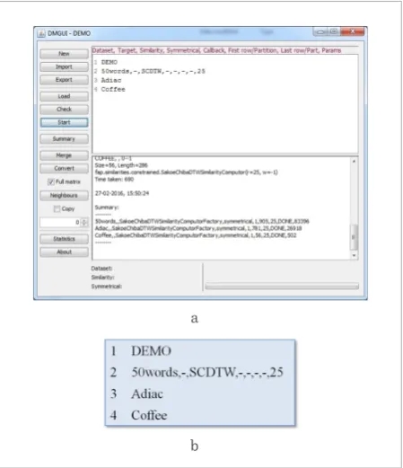
Application 2. DMGUI. To speed up some of our research efforts, another dedicated Java application was developed (within a seminar paper in doctor-al studies, similarly as the in case of SCVGUI). The aim of the DMGUI (Distance Matrix GUI – Fig. 7a) program is to provide a flexible and easy-to-use inter-face for calculating distance matrices relying on the services of our FAP library. Similarly as in the case of SCVGUI, the input for this application is a specifica-tion of one or more commands for generating distance matrices. The first line of the specification is reserved for its name. Each of the following lines represents a command for generating a single distance matrix (or just a part of a matrix).

An example of DMGUI program input specification is presented in Fig. 7b. The name of this specifica-tion, which contains descriptions of three commands for generating distance matrices, is DEMO. The first command will generate a (lower) triangular matrix of distances between the time series of the 50words

dataset using the DTW similarity measure con-strained with the Sakoe-Chiba band (SCDTW). The width of the warping window is set to 25% of the time

series’ length. The other two commands use the same attributes as the first one, therefore only the names of the datasets (Adiac and Coffee) must be provided. To further speed up the experiments with the kNN classifier, apart from calculating distance matrices, DMGUI is enabled to produce matrices of nearest neighbors, too. The i-th row of such a matrix contains all the time series of the given dataset (except the i-th series) sorted by their distance from the i-th series: the first element of the row is the most similar and the last one is the least similar.

Figure 7

Graphical User Interface for generating distance matrices: (a) DMGUI; (b) a DMGUI program

Figure 8. Comparison of the results obtained with SCVGUI and with its extension

a

b

(9)

257

Application 3. An extension of SCVGUI. As a part of a student paper in the Data Mining seminar (sec-ond and third year elective course, Bachelor stud-ies of Computer science), aimed at familiarizing the students with the basic concepts of time-series data mining through utilizing the FAP library, the SCVGUI program was extended with the ability of directly set-ting the size of the Sakoe-Chiba band (rather than determining it using the tuning algorithm described in [6]). This extended version of the application was then used to investigate the influence of the Sa-koe-Chiba band on the 1NN classifier in the case of the DTW distance measure by examining the classifi-cation accuracy for different warping window widths. The experiments consisted of evaluating 10-fold stratified cross-validations using different warping window widths in range from 10% to 1% of the length of time series with (absolute) steps of 1 for several datasets from the UCR Time Series Classification Ar-chive. The obtained smallest warping window widths which gave the best accuracy were compared with the values obtained in [21]. The results of the comparison are shown in Fig. 8.

Figure 8

Comparison of the results obtained with SCVGUI and with its extension

Application 4. Time-series reconstruction. Many tasks of machine learning and data mining are affect-ed by the issues relataffect-ed to large datasets and high-di-mensional data. These problems are known as the

curse of dimensionality and they can deteriorate the performance of standard algorithms. In the field of time-series data mining, a common approach to over-come this phenomenon is to transform the data into a lower-dimensional representation while retaining the essential properties of the original series.

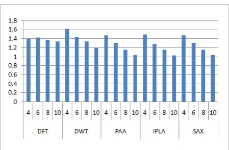
The topic of a seminar paper within doctoral studies was to investigate which representations are the most suitable for reconstructing the original time series and to find those distance measures that adapt well to the reconstructed data [17]. The analysis encom-passed 85 datasets from the UCR Time Series Clas-sification Archive [3] in combination with several time-series representations (DFT, DWT, PAA, Index-ible PLA and SAX) in four different dimensions (4, 6, 8 and 10) and a number of distance measures (L½, L1,

L2, L∞, unconstrained DTW, LCS, EDR and ERP). In order to determine to what extent the recon-structed time series differ from the original ones, the reconstruction accuracy was calculated as the

root-mean-square-deviation (RMSD), i.e. the Euclid-ean distance divided by the square root of time series dimensionality. The effectiveness of distance meas-ures is calculated in a similar manner: as the RMSD between the distances of the original and the recon-structed series (denoted as SMRE – Similarity Meas-ure Reconstruction Error). The averaged values of RMSD and SMRE are presented in Fig. 9 and Fig. 10, respectively. The analysis of the obtained results has shown that the most unstable time-series representa-tion is DFT. Furthermore, while the elastic distance measures are less adaptive to DFT reconstruction than Lp norms, they produced better results for all the

other representations.

Figure 9

Averaged RMSD values

Figure 9. Averaged RMSD values

Figure 10. Averaged SMRE values

CD4 CD8 CD3 CD4/CD8

EDR 0,49648 0,480403 0,46819 0,43032

LCS 0,51756 0,44148 0,44705 0,49334

DTW 0,46565 0,45625 0,44967 0,44077

ERP 0,41508 0,42748 0,45057 0,48232

(a) (b)

(10)

Even though some representation techniques exist-ed in FAP before this application, during this project they were revised and optimized. In addition, several fundamental representation techniques were imple-mented, making FAP’s repository of representations more comprehensive.

Application 5. Medical domain. Another student’s seminar work and paper within the Data Mining

course was performed in a specific medical area. The topic of this paper is analyzing medical records of pa-Figure 10

Averaged SMRE values

CD4 CD8 CD3 CD4/CD8

EDR 0,49648 0,480403 0,46819 0,43032 LCS 0,51756 0,44148 0,44705 0,49334 DTW 0,46565 0,45625 0,44967 0,44077

ERP 0,41508 0,42748 0,45057 0,48232

(a) (b)

Figure 11. Analyzing medical records using FAP

tients with HIV infection using different similarity measures by FAP. Two classes of PI/NRTI (protease inhibitors / non-nucleoside reverse transcriptase

in-hibitor) therapies were applied on patients and four

kinds of recovery indicators were inspected (number of CD3, CD4, and CD8 T cells and the CD4/CD8 ratio). The examined data were extracted from the database of the Infectious Diseases Clinic (Clinical Centre of Vojvodina) containing medical records of 136 pa-tients with HIV infection (Fig. 11a). The data were

Figure 11

Analyzing medical records using FAP

CD4 CD8 CD3 CD4/CD8

EDR 0,49648 0,480403 0,46819 0,43032 LCS 0,51756 0,44148 0,44705 0,49334 DTW 0,46565 0,45625 0,44967 0,44077 ERP 0,41508 0,42748 0,45057 0,48232

(11)

259

first transformed into time series to be evaluated with the FAP framework. After that, these time series were analyzed using the SCVGUI application.

Four time series were created for every patient, one for each recovery indicator. The time series were la-beled based on the type of the applied therapy and placed in the appropriate dataset (CD3, CD4, CD8, or CD4/CD8). The obtained datasets were analyzed by applying three different stratified cross-validation ex-periments using SCVGUI: 2-fold, 5-fold, and 10-fold. The average values of the acquired error rates are pre-sented in Fig. 11b.

The experiments were performed using the 1NN classifier in combination with the unconstrained ver-sions of the four most commonly used elastic distance measures (DTW, LCS, EDR, and ERP). The objective of this experimental setup was to explore to what ex-tent the extracted time series depend on the applied therapy and to identify the most appropriate distance measure.

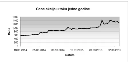
Application 6. Financial domain. The sixth exam-ple of using FAP in an educational setting is a seminar paper that was done within the course Artificial In-telligence 2. This work investigates the possibility of using techniques of time-series analysis in predicting the change of stock prices based on one-year history. The raw data (stock price changes of the Nikola Tes-la Airport in the period from 18 June 2014 to 17 June 2015 – Fig. 12) were downloaded from the Belgrade Stock Exchange’s website (http://www.belex.rs). Using the sliding window algorithm, the raw time se-ries were split into three sets of subsese-ries of the same length. The obtained subseries were labeled 1, 0 or -1, depending on whether the price increased, remained the same or decreased. The labels of the n-th (n=1,2,3)

set were determined based on stock price changes n

days in advance. The obtained datasets were analyzed using SCVGUI by applying three different stratified cross-validation experiments using SCVGUI (2-fold, 10-fold, and LOO) and the following distance mea-sures: L1, L2, DTW, and ERP.

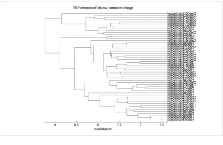
Application 7. Psychological domain. The last exam-ple is devoted to a master’s thesis [8], developed inten-sively using FAP, and it is related to research papers [16] and [18]. The subject of this thesis is analyzing log file data obtained from SAM experiments using the FAP framework in order to find the best distance measure. Three types of time series were extracted from the raw data: the first type describes the distance of the object from the starting point, the second type represents information about acceleration, and the third one specifies the deviations from the ideal trajectory (the shortest possible path). In [16], by applying hierar-chical clustering on distance matrices (generated for these time series using the DTW, EDR and ERP dis-tance measure) the ERP measure was selected as the most appropriate candidate to distinguish between the two types of navigators (i.e. “fast” and “accurate” navigators). An example of the clustering for the ERP measure is presented in Fig. 13 (taken from [16]). Due to the fact that the results in [16] were not good enough to draw reliable reliable conclusions, addition-al examinations were needed. These extended exper-iments were conducted within this thesis [8]. In the first step, time series were labeled based on the type of the navigator they belong to (1 – “fast”, 2 – “accurate”). After that, the datasets were analyzed with SCVGUI using 2-fold, 5-fold and 10-fold stratified cross-valida-tion and the DTW, EDR, and ERP measures.

The tracks in the SAM experiments are of different length and complexity. Furthermore, various nav-igators complete the same track in different times. Therefore, the extracted time series are not of the same length. In the second phase of the experiments, the time series were scaled using linear interpolation. Using the time series prepared in this manner, the ex-periments were repeated with the following distance measures: DTW, LCS, EDR, ERP, L1, L2, L½, and L∞. The results showed that that different distance mea-sures are best suited for different types of time series (distance, acceleration, deviation), but DTW gen-erally gives the best overall outcomes, regardless of whether the time series are scaled or not.

Figure 12

(12)

5. Conclusion

In this paper, we have described our Framework for Analysis and Prediction in which we intend to incor-porate all main concepts of time-series data mining and analysis, like similarity measures, representa-tions, pre-processing, classification, methods for evaluating the performance of classifiers and other functionalities. Furthermore, we have presented its application as an auxiliary tool in teaching comput-er science at all three levels of univcomput-ersity education (bachelor, master’s and doctoral studies).

Figure 13

A dendrogram for hierarchical clustering for an ERP distance matrix

Since the study program of Informatics at the De-partment of Mathematics and Informatics, Faculty of Sciences, University of Novi Sad, offers elective sem-inars and courses related to machine learning and data mining, and since the students, as part of their obligations, have to realize practical projects, FAP has proved to be an effective and suitable assisting tool. In addition, the students can choose to utilize our frame-work in carrying out experiments for the purpose of their undergraduate and master theses in different domains. Our positive experiences encourage us to believe that FAP can be useful for educational pur-poses in many other institutions as well.

References

1. Aggarwal, C. C. Data Mining: The Textbook. Springer Publishing Company, Incorporated, 2015. https://doi. org/10.1007/978-3-319-14142-8

2. Box, G. E. P., Jenkins, G. M., Reinsel, G. C., Ljung, G. M. Time Series Analysis: Forecasting and Control. 5th Edi-tion, John Wiley & Sons, Inc., Hoboken, New Jersey, 2015. https://doi.org/10.1111/jtsa.12194

3. Chen, Y., Keogh, E., Hu, B., Begum, N., Bagnall, A., Mueen, A., Batista, G. The UCR Time Series Classifi-cation Archive. 2015. http://www.cs.ucr.edu/~eamonn/ time_series_data/

(13)

261

5. Deza, M. M., Deza, E. Encyclopedia of Distances, 2nd Edition. Springer, Berlin, Heidelberg, 2013. https://doi. org/10.1007/978-3-642-30958-8

6. Ding, H., Trajcevski, G., Scheuermann, P., Wang, X., Keogh, E. Querying and Mining of Time Series Data: Experimen-tal Comparison of Representations and Distance Mea-sures. Proceedings of the VLDB Endowment, 2008, 1(2), 1542-1552. https://doi.org/10.14778/1454159.1454226 7. Esling, P., Agon, C. Time-Series Data Mining. ACM

Com-puting Surveys, 2012, 45(1), Article No. 12. https://doi. org/10.1145/2379776.2379788

8. Fodor, L. Analiza i identifikacija pogodnih mera sličnosti podataka vremenskih serija psiholoških eksperimenata. University of Novi Sad, Serbia, 2013.

9. Geler, Z. Role of Similarity Measures in Time Series Anal-ysis, University of Novi Sad, Serbia, 2015.

10. Giusti, R., Batista, G. E. A. An Empirical Comparison of Dissimilarity Measures for Time Series Classifica-tion. 2013 Brazilian Conference on Intelligent Systems (BRACIS), Fortaleza, Brazil, 2013, 82-88. https://doi. org/10.1109/BRACIS.2013.22

11. Grossmann, W., Rinderle-Ma, S. Data Mining for Tem-poral Data. In Fundamentals of Business Intelligence. Springer, Berlin, Heidelberg, 2015, 207-244. https://doi. org/10.1007/978-3-662-46531-8_6

12. Han, J., Kamber, M., Pei, J. Data Mining: Concepts and Techniques, 3rd Edition. Elsevier, 2012. https://doi. org/10.1007/978-1-4419-1428-6_3752

13. Keogh, E., Chakrabarti, K., Pazzani, M., Mehrotra, S. Lo-cally Adaptive Dimensionality Reduction for Indexing Large Time Series Databases. In Proceedings of the 2001 ACM SIGMOD International Conference on Manage-ment of Data, ACM, New York, NY, USA, 2001, 151-162. https://doi.org/10.1145/376284.375680

14. Keogh, E., Ratanamahatana, C. A. Exact Indexing of Dynamic Time Warping. Knowledge and Information Systems, 2005, 7(3), 358-386. https://doi.org/10.1007/ s10115-004-0154-9

15. Kirchgässner, G., Wolters, J., Hassler, U. Introduction to Modern Time Series Analysis, 2nd Edition. Springer, Berlin, Heidelberg, 2013. https://doi.org/10.1007/978-3-642-33436-8

16. Kurbalija, V., von Bernstorff, C., Burkhard, H. D., Nacht-wei, J., Ivanović, M., Fodor, L. Time-Series Mining in a Psychological Domain. Proceedings of the Fifth Bal-kan Conference in Informatics (BCI’12), ACM Press, New York, New York, USA, 2012, 58-63. https://doi. org/10.1145/2371316.2371328

17. Kurbalija, V., Bratić, B. Time Series Reconstruction Anal-ysis. 2016 IEEE 8th International Conference on In-telligent Systems (IS), IEEE, 2016, 771-777. https://doi. org/10.1109/IS.2016.7737400

18. Kurbalija, V., Ivanović, M., von Bernstorff, C., Nachtwei, J., Burkhard, H. D. Matching Observed with Empirical Real-ity–What You See Is What You Get? Fundamenta Infor-maticae, 2014, 129(1-2), 133-147. https://doi.org/10.3233/ FI-2014-965

19. Kurbalija, V., Ivanović, M., Budimac, Z. Case-Based Curve Behaviour Prediction. Software: Practice and Experi-ence, 2009, 39(1), 81-103. https://doi.org/10.1002/spe.891 20. Kurbalija, V., Radovanović, M., Geler, Z., Ivanović, M. A

Framework for Time-Series Analysis. In Dicheva, D., Do-chev, D. (Eds.), Artificial Intelligence: Methodology, Sys-tems, and Applications. AIMSA 2010. Lecture Notes in Computer Science. Springer, Berlin, Heidelberg, 2010, 6304, 42-51. https://doi.org/10.1007/978-3-642-15431-7_5 21. Kurbalija, V., Radovanović, M., Geler, Z., Ivanović, M.

The Influence of Global Constraints on Similarity Mea-sures for Time-Series Databases. Knowledge-Based Systems, 2014, 56, 49-67. https://doi.org/10.1016/j.kno-sys.2013.10.021

22. Laxman, S., Sastry, P. S. A Survey of Temporal Data Mining. Sadhana, 2006, 31(2), 173-198. https://doi. org/10.1007/BF02719780

23. Marteau, P. F. Time Warp Edit Distance with Stiffness Adjustment for Time Series Matching. IEEE Transac-tions on Pattern Analysis and Machine Intelligence, 2009, 31(2), 306-318. https://doi.org/10.1109/TPAMI.2008.76 24. Mitrović, D., Ivanović, M., Geler, Z. Agent-Based

Distrib-uted Computing for Dynamic Networks. Information Technology and Control, 2014, 43(1), 88-97. https://doi. org/10.5755/j01.itc.43.1.4588

25. Mitsa, T. Temporal Data Mining. Taylor & Francis, 2010. https://doi.org/10.1201/9781420089776

26. Serrà, J., Arcos, J. L. An Empirical Evaluation of Simi-larity Measures for Time Series Classification. Knowl-edge-Based Systems, 2014, 67, 305-314. https://doi. org/10.1016/j.knosys.2014.04.035

27. Wang, X., Mueen, A., Ding, H., Trajcevski, G., Scheuer-mann, P., Keogh, E. Experimental Comparison of Representation Methods and Distance Measures for Time Series Data. Data Mining and Knowledge Dis-covery, Springer US, 2013, 26(2), 275-309. https://doi. org/10.1007/s10618-012-0250-5

28. Yin, H., Yang, S., Ma, S., Liu, F., Chen, Z. A Novel Parallel Scheme for Fast Similarity Search in Large Time Series. China Communications, 2015, 12(2), 129-140. https://doi. org/10.1109/CC.2015.7084408

29. Zaki, M. J., Meira, W. Jr. Data Mining and Analysis: Fun-damental Concepts and Algorithms, Cambridge Univer-sity Press, New York, 2014.