DNA Microarray Data Analysis and Mining: Affymetrix Software Package and In-House Complementary Packages

(1)

University of New Orleans Theses and

Dissertations Dissertations and Theses 12-19-2003

DNA Microarray Data Analysis and Mining: Affymetrix Software

Package and In-House Complementary Packages

Lizhe Xu

University of New Orleans

Follow this and additional works at: https://scholarworks.uno.edu/td

Recommended Citation Recommended Citation

Xu, Lizhe, "DNA Microarray Data Analysis and Mining: Affymetrix Software Package and In-House Complementary Packages" (2003). University of New Orleans Theses and Dissertations. 60. https://scholarworks.uno.edu/td/60

This Thesis is protected by copyright and/or related rights. It has been brought to you by ScholarWorks@UNO with permission from the rights-holder(s). You are free to use this Thesis in any way that is permitted by the copyright and related rights legislation that applies to your use. For other uses you need to obtain permission from the rights-holder(s) directly, unless additional rights are indicated by a Creative Commons license in the record and/or on the work itself.

(2)

DNA MICROARRAY DATA ANALYSIS AND MINING

AFFYMETRIX SOFTWARE PACKAGE AND

IN-HOUSE COMPLEMENTARY PROGRAMS

Submitted to the Graduate Faculty of the University of New Orleans

in partial fulfillment of the requirements for the degree of

Master of Science in

The Department of Computer Science

by Lizhe Xu

B. S., Ocean University of China, 1986

M.S., Université d’Aix-Marseille II, Marseille, France, 1989 Ph. D., Université Pierre et Marie Curie, Paris, France, 1994

(3)

ii

Acknowledgment

I want to thank Professor Seth Pincus for giving me the opportunity to work on this interesting project, and for the work he did in microarray experimental design and cell

culture resources. In particular, Seth was very helpful and supportive throughout the whole process.

I would also like to thank:

Dr. Jason Giardina for sample preparation

Jill Schurr for microarray hybridization and advice regarding the Affymetrix software Holly Guevara and Alyson Moll for data analysis

I particularly appreciate the help of Padmanabhan Mahadevan, Brent Fodera and Yachi Yang for reviewing and correcting my thesis.

I also wish to express my gratitude to Professor Mahdi Abdelguerfi, Professor Bin Fu, Professor Stephen Winters-Hilt and Professor Eduardo Kortright for their support in this

work.

(4)

iii

List of Figures, Tables and Codes

Figure 1. The four corner stones of System Biology 4

Figure 2.Affymetrix Manufacturing Technology 7

Figure 3. Two Repeat Schemas in microarray studies 12

Figure 4. Affymetrix gene expression analysis software package 19

Figure 5. The sampling schema of the time course study 21

Figure 6. Affymetric microarray study process. 22

Figure 7. MAS data analysis output format. 24

Figure 8. Time course study comparison analysis schema. 25

Figure 9. Output of the Mann-Whitney test in DMT 26

Figure 10. The difference between MAS Scaling and Normalization 29 Figure 11. Screen shot of HCL of experiments in Tiger MeV 38

Figure 12. Screen shot of PCA analysis in Tiger MeV. 39

Figure 13. Screen shot of the Perl Script II IS-UN-GL.pl. 41

Figure 14. The Structure of the in-House Database. 45

Figure 15. Screen shot of Probe Data. 46

Figure 16. Example of pattern search in Probe-Data. 48-49

Figure 17. Screen shot of the General Layout of Probe-Set. 50 Figure 18. Screen shot of the layout of Search Entry in Multiple Fields in Probe-set. 51 Figure 19. Screen shot of design report of the in-house database. 52 Figure 20. Screen shot of the layout of General List View in Probe-Set. 53

(7)

vi

Script I. Parallel-Analysis.pl, the tool for parallel DMT analysis. 59 Scrip II. IS-UN-GL.pl, the modification of Script I, which will do the union as well as

intersection of selected gene lists. 63

(8)

vii

Abstract

Data management and analysis represent a major challenge for microarray studies.

In this study, Affymetrix software was used to analyze an HIV-infection data. The

microarray analysis shows remarkably different results when using different parameters

provided by the software. This highlights the fact that a standardized analysis tool,

incorporating biological information about the genes is needed in order to better interpret

the microarray study. To address the data management problem, in-house programs,

including scripts and a database, were designed. The in-house programs were also used to

overcome problems and inconveniences discovered during the data analysis, including

management of the gene lists. The database provides rapid connection to many online

public databases, as well as the integration of the original microarray data, relevant

publications and other useful information. The in-house programs allow investigators to

(9)

Introduction

Biological Background

The cell is the basic building block of a free-living organism. No matter how simple or

how sophisticated the organism is, every cell contains the complete organism’s hereditary

information which is comprised of a set of genes. For a given species with only a few exceptions,

each of its cells contains identical genes, and the whole set of genes forms the genome of that

species. The number of genes varies from hundreds to tens of thousands depending on the

organism. In the human genome, the latest estimates from gene-prediction programs suggest that

there might be 24,500 or fewer protein-coding genes [2]. The mystery of life in a living cell

resides in the function of its genes and their products. For a multiple-cell organism, cells have a

variety of functions. The biological difference between the cells is achieved by an “on/off

toggle” to control which genes are expressed in a cell and a “volume control” to manage the

level of expression of particular genes as necessary [3]. The number and the level of these

“turned-on” genes in a cell form the so-called gene expression profile, which determines the

biological properties of that cell.

In humans, all the genetic information is contained within a set of deoxyribonucleic acid

(10)

expression is usually composed of two separate steps: transcription and translation (see Fig. 1).

The former denotes transcribing the genetic information contained in a gene into messenger

RNA (mRNA, ribonucleic acid) molecules. The total information (qualitative and quantitative)

of mRNA generated from a given genome is called the Transcriptome. Translation is

converting the coding information in the transcriptome into the corresponding proteins, which in

turn perform most of the critical functions of cells. The total information about the proteins and

their functions are called Proteome and Metabolome respectively (see Fig. 1). The integration of

these four layers (genome, transcriptome, proteome and metablolome) of studies, termed

'Systems Biology,' can tackle the complexity of biological systems by gathering and

incorporating all the available information into one comprehensive model [4]. As a result, the

study of gene expression can be conducted at two different levels: mRNA and protein. Figure 1. The four corner stones of System Biology, (System Biology is an emergent field that

(11)

Traditional methods in molecular biology generally work on a “one gene or few genes in one

experiment” basis. This means that we can only study a small part of the cellular functions at a

time, and it is very difficult to obtain the whole gene expression profile of the cell. However, it is

obvious that the entire gene expression information in a cell is needed to better understand its

function, since thousands of genes (usually just a fraction of human genome) inside the cell are

working in a complicated and orchestrated way to support the organism’s biological function and

to make the cell perform its normal role. In order to better understand the extreme complexity of

living system, a more powerful research tool is required for cellular gene expression studies.

The DNA microarray, also known as genome chip, biochip, DNA chip, gene array and

GeneChip® (a registered trademark owned by Affymetrix, Inc, CA) is an approach provided to

accomplish this quest. DNA microarray is currently one of the fastest developing tools in the

biological sciences. This technology promises to monitor a specimen’s entire genome on a single

chip in a single experiment. As a result, investigators can have a more precise and complete

knowledge of the interactions among the thousands of genes expressed in a cell simultaneously.

DNA Microarrays

Each DNA molecule is made up of four different nucleotide bases, [adenine (A), thymine

(T), guanine (G), and cytosine (C)], that are linked end to end. The order of the 4 bases (A, G, C,

T) determines the contents of the genetic information of DNA, either directly (the sequences of

the bases encodes the genes) or indirectly (the fragment of the DNA can play a regulatory role).

In general, two DNA molecules can form a very stable structure through the complementarity of

their bases, the famous “Double Helix”. That is, adenine being the complement of and always

pairing with thymine, and guanine being the complement of cytosine. This natural base-pairing

(12)

sequences mix together and one finds its complement, such as, the sequence A-G-C-T-T-G-G

and its complementary sequence T-C-G-A-A-C-C, the two sequences will lock together by

base-pairing. In molecular biology, this is called hybridization. It is complementary base-pairing or

hybridization that forms the foundation of the DNA microarray. RNA molecule follows the same

basic rules of base-pairing as DNA, but with a substitution of uracil (U) for T. The base pair for

RNA is A and U or G and C. One RNA molecule can also hybridize with a DNA molecule

based on the base-pairing rule.

In The American Heritage Dictionary, “array” is defined as “to place in an orderly

arrangement”. DNA microarrays are small, solid supports onto which the sequences from

selected thousands of different genes are attached at fixed locations [3]. The solid supports can

be nylon membranes, glass microscope slides or silicon chips. Genes are printed (similar

mechanics to an ink-jet printer), spotted by high-speed and precision robotics, or synthesized

directly onto the support (see Fig. 2). These immobilized genes are used to capture the test DNA

samples based on base-pairing rules. According to the nomenclature recommended by B.

Phimister of Nature Genetics, these immobilized sequences are called “probes” and those

sequences captured by probe are the “target” [5]. The probes in a microarray can be DNA, cDNA

(DNA copied from RNA) or synthetic oligonucleotides. Usually, probes of DNA or cDNA can

be 500 to 5000 bases long, whereas the size of an oligonucleotide microarray (Oligo-Array)

probe is only 20 to 80 bases long. Due to the small size of an oligonucleotide probe, these arrays

can hold more gene probes per unit space. As a result, the Oligo-Array is a high density

microarray (up to tens of thousands of probes in one microarray) compared to DNA or cDNA

(13)

DNA microarray permits the study of cellular gene expression at the transcription level.

In other words, the microarray can detect the existence and measure the quantity of cellular

mRNA. To achieve the qualitative and quantitative analysis, the sample of cells must be

pre-treated according to the following steps:

1) RNA extraction. The first step is to isolate RNA from cells by eliminating

all other cellular components. Depending on the experimental design and

protocol, the isolated RNA can be further purified to get the only mRNA

prior to the second step.

Figure 2. Affymetrix Manufacturing Technology, Affymetrix uses a unique combination of photolithography and combinatorial chemistry to manufacture GeneChip® Arrays (from Affymetrix.com)

2) Fluorescent labeling of the target RNA or mRNA. This allows detection

and quantification of gene expressions by measuring the hybridization

(14)

The labeling process can be simply one step of reverse transcription of RNA to cDNA,

during which the cDNA are labeled, or it may be composed of multiple reactions. In the

Affymetrix microarray for example, there are two sub-steps in this process: reverse transcription

of RNA to cDNA without labeling, then followed by in vitro transcription of cDNA to cRNA

labeled with biotin (Affymetrix manual, CA). It is not the intention of this thesis to cover the

sample preparation of DNA microarray. However, based on how the samples are labeled, DNA

microarray can be separated into two groups: single-color or color microarray. In the

two-color system, two samples to be compared (for example, disease versus healthy, or non-treatment

sample versus treatment sample, etc) are labeled individually with different fluorescent dyes, and

then hybridized to one microarray. The same gene in the two samples will compete with each

other to hybridize with the corresponding probe on the array. The relative expression levels of

genes in one sample are determined by the signal densities captured in the corresponding

fluorescent channel. The ratio of the signals in two channels of a given probe represents the

difference of the corresponding gene in the two samples under study. In the one-color microarray,

only one labeled sample can be used to hybridize with one microarray. After the image capture,

the relative abundance of transcripts in the sample is obtained by image processing software

which contains the algorithms for spot identification, local background determination and

background-subtracted hybridization signal density calculation [6]. Comparisons between groups

are then made on separate chips, thus requiring greater standardization and normalization.

Oligo-Arrays usually use a single-color labeling system. Affymetrix only produces Oligo-Oligo-Arrays and as

a result, its sample preparation uses single color method. Affymetrix’s software package is

dedicated to data analysis of one-color microarrays.

(15)

levels: mRNAs and proteins. DNA microarray provides the research tool to scientists at the

mRNA level. Another technology called the protein chip, is the approach to investigate at the

protein level. The protein chip is another rapidly developing research technology. For example, a

recently finished strategic report conducted by BioPerspectives (www.biotechinsights.com)

estimates that the sale of protein chips will be increased from $76 million in 2001 to $700

million in 2006 [7]. The protein chip shares a similar technique as the DNA chip, but instead of

DNA probes, it uses proteins or peptides immobilized on a surface to capture other proteins.

Through the protein-protein or protein-ligand interaction, protein chips realize the analysis of

thousands of proteins expressed in a cell in parallel. Although the topic of the protein array is out

of the scope of this thesis, it is worth noting that the protein microarray faces the same challenges

in its data analysis and data mining as the DNA microarray. In other words, a better data analysis

and data mining strategy for DNA microarray will certainly benefit the protein microarray and

vice versa.

Benefiting from the powerful microarray technology, scientists can now determine

simultaneously the relative expression levels of all the genes represented in the array from only

one experiment. Microarrays are currently available that claim to probe most, if not all, genes in

the human genome. In addition to gene expression analysis, the microarray technology has been

widely used in many other fields, such as, gene discovery, sequence identification, disease

(16)

Microarray Data Analysis and Mining

Challenge of Microarray Data Analysis

The ability of the microarray to address thousands of genes at a time is its strength, as

well as its weakness: the data analysis and data mining are problematic. Since one microarray

experiment can generate tens of thousands of data points representing the expression levels of the

genes it probes, it is impossible to manipulate and analyze these data manually. Microarray data

analysis requires

1) carefully designed computational tools to manage the data, including but not

limited to data storage, gene annotations, probe and/or gene sequences,

biochemical pathway and a variety of other biological knowledge about the genes

immobilized on the array;

2) robust statistical and biological analysis methods (requiring computer support for

semi- or fully automatic performance) to turn the numerical data of a gene in the

array into a biologically meaningful interpretation.

From the initial cells to the final data, there are many intermediate preparation steps for a

gene expression study, which can impart uncertainties, called technical variances, to the result.

Because of technical variances, the results of microarray studies from the same cohort of cells

can differ from one experiment to the next. As the averages of signal among replicates typically

(17)

microarray study. Moreover, replicate arrays allow the use of formal statistical methods for the

downstream data analysis. So, there are generally at least two arrays (duplicate) for one

experiment. Meanwhile, microarray studies are generally used to determine differential gene

expression between identical cells subjected to different stimuli or between different cellular

phenotypes or developmental stages. These kinds of differences generated from the initial

samples are called biological variances. One set of data from a single array only gives gene

expression information at a given moment. It is impossible to get a difference in mRNA

expression levels from a single array. At least one other array from a different time point or

representing a different treatment condition is required to evaluate the expression changes. For a

simple microarray study, there are at least two experimental conditions with replicates for each

condition (meaning at least 2 x 2 microarrays per study). Moreover, a living cell has the ability to

rapidly respond to surrounding environmental or internal changes (for example different stage of

cellular life or development cycle). The expression of cellular genes is changing dynamically and

continuously over time. A simply array study with only two conditions cannot catch the

changing details of gene expression, which can be important for a given study. A proper and

careful experimental design can solve this problem by multiple sampling over time. Sampling

over a relative long period of time is called “time course study”, which is a common design used

in microarray studies.

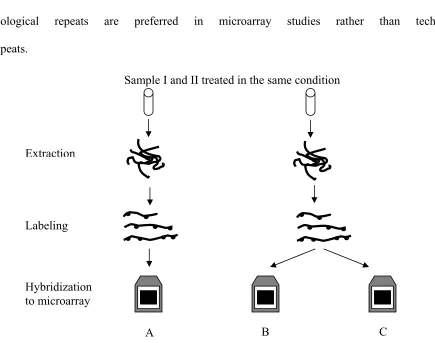
It is worth noting that there are two kinds of replicates in gene expression studies. The

one starting from the initial point of the microarray experiment is called a biological repeat. If

the same sample preparation is used to hybridize with different arrays, this kind of replicate is

called a technical repeat. For example, the relationship of A - B and A – C is considered a

(18)

relevant to display the technical variances of the steps it covers. Only the biological repeat can

reveal both the biological variances and the technical variances of the whole experiment. The

biological repeat also gives more analysis power to the downstream statistical tools. This is why

biological repeats are preferred in microarray studies rather than technical

repeats.

With multiple microarrays in one study, we must compare one with another (between

replicates and between conditions) to reveal gene expression changes. In order to compare data

from two arrays, a mathematical technique called normalization must be applied to the data of

each array. The aim of the normalization is to minimize discrepancies due to the technical

variables including but not limited to sample preparation, RNA quantification, hybridization

conditions, or image capture. For example, if the scanning time for two arrays is slightly

different during the image capture step, the array scanned for a longer time will have overall Sample I and II treated in the same condition

Extraction

Labeling

Hybridization to microarray

A B C

(19)

signal density higher than the array scanned for a shorter time. It is obvious that incorrect results

will be obtained if the two are compared without normalization. Depending on the experimental

design, there are several useful techniques for normalization. For a single color array, the most

commonly used method is to divide the signal of each gene by the mean or median of total

measured intensity in its array. The reason is that the mean or median of an array is an index of

relative intensity (or baseline) of the given array. An alternative method is to use the mean or

median of selected housekeeping (HK) genes in the array to serve as the index of relative

intensity. The assumption underlying this method is that the housekeeping genes are a set of

predefined genes required for fundamental cellular processes in a wide range of cell types and

tissues and thus whose expression should be constant across the conditions of microarray studies

[8]. Besides these two methods, there are several others such as using spiked positive controls for

normalization baseline and intensity-dependent normalization[6, 8]. Normalization is the first

step of microarray data analysis after image processing. This starting point fixes the tone of the

following analysis and more or less determines the final output of the analysis.

Following normalization, data are analyzed to identify genes that are differentially

expressed between the experimental conditions. Generally, the majority of genes presented on a

microarray are invariant across the conditions under study, except in some customized arrays

which contain only the genes of interest that are likely to vary. The first step of analysis is to

filter out these invariants. Besides some user-defined filters, for example a requirement of

minimum value on normalized signal, statistic tests are the most useful tools in this step.

Depending upon the distribution of the data, users can apply either parametric or non-parametric

statistical tests. With hundreds to thousands of genes in an array, the whole data set after log

(20)

for two-condition experiments and ANOVA (Analysis of Variance, 1-way or 2-way) for

multiple-condition (time course) studies. During these statistic tests, user-defined cutoff values

allow the scientists to tune the analysis stringency to achieve the desired balance of sensitivity

and specificity. This fact results in a certain amount of flexibility (and arbitrariness) when

interpreting the microarray data. The final list of “genes whose expression is altered” generated

from a gene expression study may change as the analysis parameters or cutoff values are

modified. Moreover, since the number of tests greatly exceeds the number of samples (tens of

thousands of probes per sample for an array), microarray data analysis really pushes the standard

statistical methods for multiple comparison to the limit of their utility [4]. As an unusual

statistical case, the survival list passed through the traditional statistical tests will contain a

considerable amount of false positive genes (type I error: invariant genes being selected by error).

To mitigate the type I error in microarray analysis, several multiple test corrections (MTC) have

been proposed, for example: Bonferroni correction; Bonferroni Step-down [9], Westfall-Young

permutation [10] and Benjamini and Hochberg’s False Discovery Rate (FDR) [11]. The order of

these methods represents their stringency, with Bonferroni correction being the most

conservative method. It gives the least false positive genes among the four methods but can filter

out some true variant genes (type II error: variant genes being dropped by error). In contrast FDR

generates the least type II error but has more type I error. The choice of MTC method is a

study-specific decision in microarray data analysis. Therefore, genes with biologically relevant

expression changes may not be effectively captured with statistical tests. This continues to be an

active area of statistical research. This is why non-statistical approaches must be used in

conjunction with statistical methods to interpret and validate the biological importance of the

(21)

The next step is to classify the genes that are statistically significant into different groups

based on their expression patterns. This can be realized by several analysis and visualization

tools, including, but not limited to, SOM (Self Organizing Map), hierarchic clustering (K-means,

Gene tree, condition tree etc), and PCA (principal component analysis) [12-15].

The last step in the analysis of gene expression data is the biological interpretation of the

results, where expression profiles contribute to the functional genomics characterization of the

biological system under investigation [4]. Gene expression changes are controlled through highly

complex, non-linear interactions between proteins, DNA, RNA, and a variety of metabolites. To

find the functional relevance of expression data requires gathering and organizing a variety of

additional bioinformatics associated with the sequences that show significant changes. It also

involves correlating expression results with other types of data that can gathered as part of the

experiment, such as, genomic, proteomic, or metabolomic data (see Fig. 1) [4]. The challenges of

biological interpretation and the few tools available have made this step the bottleneck in

microarray data analysis. One fundamental difficulty is the requirement for human review and

understanding of complex types of data, scattered across a variety of sources, including online

data bases and journal publications. While most investigators rely largely on 'manual'

interpretation of results, through the review of functional annotations, pathway information, and

associated literatures, there are efforts to develop tools that would truly automate some of the

biological interpretation tasks, such as knowledge mining tools and gene network modeling and

prediction [4]. In summary, the analysis steps mentioned above form the simplified pathway for

the microarray data analysis from one gene expression study.

There are several software products available specifically designed for microarray

(22)

Institute for Genomic Research) MeV (multiExperiment Viewer v2.1 [16], free), D-Chip (free)

[17, 18] and RMA (Robust Multi-array Analysis, free) [19, 20], Affymetrix’s DMT (Data

Mining Tool) and Silicon Genetics’ GeneSpring [21] etc. Although the license of a commercial

program can cost tens of thousands of dollars for a limited time of usage, the different software

products and even the different settings within the same software product can greatly affect the

analysis results and conclusion [15]. As a result, direct techniques of biological validation

techniques, such as real time RT-PCR or analysis of specific proteins, are needed to confirm the

final results by directly measuring the mRNA or protein quantities. But, these manual laboratory

methods are time consuming and can only be applied to a small subset of the genes identified by

microarray studies.

As cited above, biological context is needed during this process to help achieve the final

results. However, since the high throughput DNA sequencing technology is advanced, vast

amounts of sequence information have been generated from difference species. For example, the

human genome project was originally planned to be a 15-year project, but completed 2 years

ahead of its schedule. During the 13 research years, 3 billion nucleotide base pairs were

sequenced, from which about 25,000 genes (this number is still changing depending on the new

prediction tools) have been identified. Among these tens of thousands of genes, only a small

number have more or less related genomic, proteomic, or metabolomic information and most of

them just have a gene name assigned [22]. In addition, some microarrays use expressed

sequence tags (EST: A short strand of DNA that is a part of a cDNA molecule and can act as an

identifier for locating and mapping genes) as probes, in which case there may be no information

other than sequence available. This means that a majority of genes in a microarray could have no

(23)

data analysis even more challenging. Indeed, the lack of information for genes creates another

application field for microarray study besides gene expression analysis. That is to determine the

function of genes, and even to identify new genes by comparing their expression profiles with

well-characterized genes (that is why the EST is used as probe in microarrays).

With all the problems accumulated from the various steps presented above, the most

challenging part of microarray data analysis is to compare two or more similar studies, especially

ones coming from different laboratories. Since the microarray technology was developed

independently from multiple sources, different microarray techniques are available in the market

vis-à-vis the number, type, sequence of probes, solid supports, sample preparations, and labeling

systems. Similar studies performed in different laboratories can use different microarray

techniques, different programs or different settings of the same program for data analysis. The

results can be widely variable, so in most cases it is problematic, if not impossible to compare

the final results between two studies. To facilitate the comparison and sharing of microarray data,

the international Microarray Gene Expression Data (MGED) Society drafted the requirement of

MIAME (minimal information about a microarray experiment) [23]. MIAME is not a strict

rulebook for microarray experiments, but provides a set of guidelines. It aims to unambiguously

interpret microarray data and to allow sharing and interpretation of raw data between different

studies [23]. The data sharing allows other investigators to assess and validate the quality of data,

further analyze, and mine the data beyond that which might be presented in an original study

[15]. Additionally, it facilitates the development of more powerful and comprehensive software

for analysis by providing real data for testing. Moreover, as there are many variations involved in

microarray studies, accumulation and sharing of data from many studies makes it possible to

(24)

thousands of microarray studies from different types of cells and tissues, at different stages of the

life cycle or in different conditions, will construct organism-level gene expression profiles which

show the dynamical changes cross time and conditions. With these precious gene expression

pictures in hand, scientists will be able to finally discover the mechanisms of life.

Affymetrix Microarray System

Affymetrix Inc (CA) is one of the earliest, most successful companies to develop

microarray technologies. To date, there are about 1400 scientific publications related to

Affymetrix’s GeneChip® [24]. The Affymetrix GeneChip®s are high density Oligo-arrays (with

length around 25), in which the probes are synthesized directly onto the supports (see picture 3).

In order to increase the sensitivity and specificity of the test, there are a set of 11-16 different

probe pairs for each gene on the chip, which cover different areas of the given gene. A probe pair

is composed of one perfect match (PM) probe and one mismatch probe (MM). The PM probe has

the complimentary sequence to the gene of interest and the signal of the PM represents the

specific hybridization. The MM probe has the same sequence as the PM, except for a homomeric

base change (A - T, or G – C) at the middle of the sequence (at the 13th position). The signal of

the MM represents non-specific hybridization. The detail of the usage of the PM and MM can be

found in the following references [4, 14, 25-27]. Affymetrix’s gene expression analysis arrays

cover the genomes of Arabidopsis; P. aeruginosa; E. Coli; yeast; C. elegans; rat; mouse and

human. Among several different chip sets of human genome, the U133 AB chip set is the newest

chip and at the time of this study, contained the highest number of genes available. The U133

AB chip set is composed of 2 chips, named U133A and U133B. The U133A chip contains 22283

known human genes (many of them having unknown biological functions). The U133B chip has

(25)

genes. The data used in this thesis was generated from this chip set in an HIV (human

immunodeficiency virus) infection study (funded by LA Board of Regents grant LEQSF

(2002-05)-DR-B-06, led by Dr Seth Pincus, Director of the Research Institute for Children). The details

of the HIV infection microarray experiments will be presented in the following section.

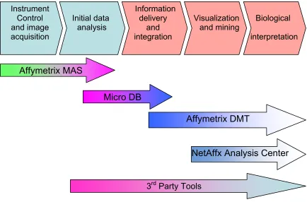
In addition to GeneChip®, Affymetrix also provides a software package, including

Microarray Suite (MAS) 5.0 [26], MicroDB [27], Data Mining Tool (DMT) 3.0 [14] and even an

online analysis tool called Affymetrix® NetAffx™ Analysis Center. These programs and tools

cover the entire gene expression experiment, from the initial chip hybridization instrument

control to final biological interpretation (see Fig. 4). During the analysis of HIV infection study,

I used all Affymetrix’s analysis tools mentioned above as well as several other programs such as

Silicon Genetics: Gene Spring [21] and Tigrs MeV [16]. The different parametric settings

(including normalization methods) of these software tools have been tested and significant

differences were obtained from different programs and different settings of the same program

[28]. The results, details of the analysis process, and the different settings of parameters will be

published elsewhere and not covered here [28]. In this thesis, I will only present a small part of

the data analysis study, which starts from the MAS and DMT analysis and ends with use of

several in-house programs, including scripts and a customized database. Both the scripts and

database have been created to overcome weakness of the Affymetrix program and to help the

investigators conduct the analysis in a fast and easy manner, as will be shown in later

(26)

HIV Infection Study

The HIV infection experiment was performed at the Research Institute for Children (RIC)

and was composed of two parts: chronic infection study and acute infection study. The first was

a simple study of gene expression, with only two conditions: persistently infected cells versus

non-infected cells. The uninfected parental cell line, designated H9, is a clonal derivative of the

Hut 78 cell line, isolated from human cutaneous T CD4+ lymphocyte. It was selected for

permissiveness for HIV-1 replication [29]. H9 cells were infected with the molecularly cloned

HIV NL4-3 [30]to obtain the persistently infected cell line H9/NL4-3 [31]. The chronic study

was performed by directly comparing the microarray data between H9/NL4-3 cells and H9 cells.

The acute infection study, although using the same two cell lines, is more complicated than the Instrument

Control and image acquisition

Initial data

analysis

Information delivery

and integration

Visualization and mining

Biological

interpretation

Affymetrix MAS

Affymetrix DMT

NetAffx Analysis Center Micro DB

3rd Party Tools

(27)

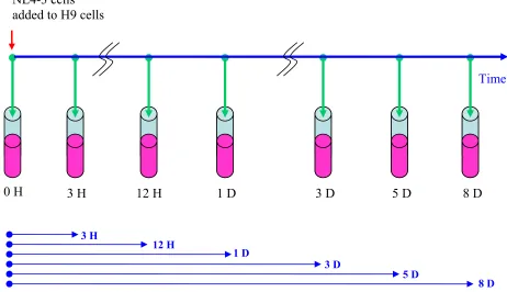
previous one. It was designed as a time course study by using H9/NL4-3 cells to infect H9 cells

and evaluating the gene expression changes in H9 cells over time. H9 cells at their mid-log phase

of growth were mixed with H9/NL4-3 cells at ratio of 50 to 1 (H9 : H9/NL4-3) and one tenth of

the mixed volume (equals to one tenth of the mixed cells) was removed immediately after the

initial mixing and at various time afterwards. Cells were washed X 2i in phosphate buffered

saline, resuspended in RNALater, and stored at –200 until ready for use. RNA was extracted

using TRIzol®,a reagent which can disrupt cells and dissolve cellular components, while

maintaining the integrity of the RNA [32]. in addition to the initial sample, other samples were

taken at 3 H, 12 H, 24 H, 3 days (D), 5 D and 8 D after the time zero (see Fig. 5).

The experiments from RNA extraction to hybridization followed exactly the Affymetrix

protocol [25] and the whole process is illustrated in 6. Thanks to the investigators (see my NL4-3 cells

added to H9 cells

Time

0 H 3 H 12 H 1 D 3 D 5 D 8 D

3 H

12 H

1 D

3 D

5 D

8 D

(28)

Acknowledgement on page 2), I started my analysis without worrying about the preparation steps

and took charge of the study just after the step of “Scan” (see Fig. 6).

For the reason I cited previously, both chronic and acute infection studies were repeated

three times independently from cell culture and cell infection to final hybridization (biological

triplicates). As a result, I obtained a total of 54 image files obtained by scanning the hybridized

chips. Each file had a size of 43 MB. They are from the U133A and U133B chip set, with each

set having two samples of chronic infection and seven samples of time course study for

triplicates per sample [2x (2+7) x 3 = 54].

Figure 6, Affymetric microarray study process (coming from [4]).

Data Analysis Schema with Affymetrix’s Programs

1) MAS (Microarray Suite 5.0) . The first step of the data analysis was to use the image

processing algorithm in MAS to analyze the received image files. MAS evaluated the whole set

(29)

“.cel” file was generated from each image file. The next step is called absolute data analysis or

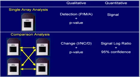
single array data analysis (see Fig. 7). The resulted “.chp” files contains both quantitative and

qualitative measurements for each probe set by incorporating the density value of its 11-16

primer pairs from the “.cel” file. The quantitative measurement shows the absolute signal value

of each probe set (obtained by evaluating all its probe pairs). The qualitative measurement is

given as a form of detection call with an associated p-value for confidence: P (Present, gene

expression above the detection threshold), M (Marginal, at the limit of detection threshold) and A

(Absent, below the detection threshold). The two measurements were calculated using different

algorithms of detection and they were independent from each other (for details please refer to

Appendix C of AMS manual [26]). The following step is the comparative analysis to compare

two conditions: experiment versus control (or baseline) (see Fig. 7). Just like in the single array

analysis, MAS uses different algorithms to generate both quantitative and qualitative

measurements. The quantitative measurement gave the signal log ratio (SLR, log base of 2) of

the two experimental conditions (experiment divided by control). For example, if SLR for one

gene is 1, it means that the expression of this gene is two fold higher in the experiment than that

in the control (up-regulated gene) since log22 = 1. If SLR is -1, it means that the expression of

this gene in the experiment is half of that in the baseline (log2 0.5 = -1, down-regulated gene).

The qualitative measurement gave the following calls with an associated p-value: I (Increase, the

gene expression is increased in the experiment compared to control); MI (marginal increase); NC

(no change); MD (marginal decrease) and D (decrease) (see Fig. 7). Both measurements are

included in the comparison analysis “.chp” file, the output of the analysis. If we start with 6

image files of microarrays (two conditions and triplicates for each condition), we will get a total

(30)

“.chp” files and 9 comparison analysis “.chp” files.

2) MicroDB. This software is used to “publish” (term used by the MicroDB) [27] the

“.chp” files to a database in order to allow the DMT program to access them and perform

statistical and clustering analysis. Affymetrix’s MicroDB can only open one data base at a time,

and each data base can hold maximum 128 “.chp” files [27].

Figure 7, MAS data analysis output formats. For a comparison analysis of duplicate per condition study, there are total 4 files as an analysis result. P: present; M: marginal; A: absent; I: increase; NC: no change; D: decrease [4].

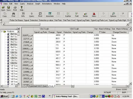
3) DMT (Data Mining Tool). In the MAS step, the data of two conditions were compared

and the detection call of I or NC or D was generated for each gene, however, no genes were

filtered out at that step. The analysis with DMT will reduce the complexity of data by filtering

out the majority of genes, keeping only the ones with statistically significant expression changes.

The DMT, just like the MAS, does not have the ANOVA (Analysis of variance) model

(31)

Once a given database, created by MicroDB, is selected in DMT parameter setting window,

DMT will have accessibility only to the “.chp” files in that data base. In other words, DMT can

access only one data base at a time. The genes with statistically significant expression changes

can be separated into two groups: up-regulated genes (expression increased in experiment or

decreased in baseline) and down-regulated genes (expression decreased in experiment or

increased in baseline). The analysis with DMT for data of two conditions has to be performed

twice in order to discover both up-regulated and down-regulated genes (simplified as up genes

and down genes afterwards). Both searches were realized with four tests based on the qualitative

and quantitative measurements of the absolute and comparison analysis.

The first test (T1) was done by using the detection call of a single array analysis to avoid

genes with A-A detection calls (absent in both experimental and –baseline conditions). When

looking for up-regulated genes, it is obvious that the genes must be present (P) in the

experimental condition, no matter what calls they have in the baseline (up-regulated gene could

be P-X but not M(marginal)-X, or A-X, where X is P or M or A in control condition, in other

words, a gene with M or A call in the experiment can not be an up-regulated gene). Using similar

reasoning, only genes having P call in the baseline can be the candidates for down-regulated

genes with a pattern of X-P, where X is P or M or A in the experimental condition.

The second test (T2) was a statistical test based on the density signals of the single array

analysis files. DMT provides two algorithms: a parametric method, the t-test and a

nonparametric method, the Mann-Whitney test, to compare two experimental conditions. Both

(32)

The third test (T3) was performed based on the detection call in the comparison analysis

files. The general rule is choosing genes with I and/or MI detection calls when looking for

up-regulated genes and genes with D and/or MD calls for down-regulated genes.

The fourth test (T4) was a fold-change-selection filter. Based upon the minimum fold

changes selected by the investigators, a different cutoff value will be determined for SLR. For

example, if at least two fold change genes are the targets, the genes passed through this filter will

have SLRs not smaller than 1 (up genes) or not greater than -1 (down genes).

(33)

Figure 9, Output of the Mann-Whitney test in DMT. The test gives both the p-value and the change direction call (up, none and down).

In a summary, T1 is based on detection call of individual array (P-M-A). T2 is a statistic

test base comparing signal densities and variation of individual genes. T3 is based on detection

call of comparison analysis (I-NC-D). T4 is a filter on fold change by using the SLR in

comparison files. The combination of these four tests will give the genes with statistically

significant changes from DMT. As we have seen, to compare two conditions, all the

corresponding single array analysis and comparison analysis “.chp” files are needed (in the HIV

study, 6 single array analysis files and 9 comparison analysis files for any two given conditions),

so all the files have to be added into the same database to allow DMT access to the data at the

(34)

Figure 10. The difference between MAS Scaling and Normalization.

Parameter Settings of Affymetrix’s Programs

Prior to single array or comparison analysis in MAS, there is an important parameter to

set: normalization, which is essential for comparing different array signals. MAS provides two

forms of normalization: Scaling and Normalization. Scaling and Normalization are mathematical

(35)

discrepancies due to technical variables [26].They will bring the average signal of the genes in

two arrays to the same level (target signal) before the comparison can be performed. The target

signal can be determined in two ways, either by users’ selection or using the average signal of

one of the two arrays that are being compared (usually using the baseline array). If the target

signal is selected by users, the signal of each gene in both arrays will be normalized in a way that

the final average signal of modified data will equal to selected value. This is the Scaling method.

If the average signal of the baseline is selected as the target value, only the data in the

experimental array will be normalized. As a result, its new average signal will be equal to that of

the baseline. This is the Normalization method (see Fig. 10). Both methods will use the

following formula to normalize the raw data.

normalized data of a given gene = its raw data x Scale Factor (SF)

where SF = Target signal / average signal of the array

Since the baseline of our pair-wise comparison was changed during the time course study,

the Normalization will cause problems for downstream analysis between these pair-wise

comparisons. So the Scaling method was chosen to normalize data in the HIV study and the

default value of MAS: 500 was used as target signal. As previously mentioned, there are two

methods to calculate the average signal of the array one based on all genes in the chip and the

other based only on some pre-selected HK genes. MAS supports both methods and Affymetrix

provides two groups of 100 HK genes for U133A and U133B separately. According to

Affymetrix’s experiments, the expression levels of these HK genes are generally constant across

(36)

Scaling were used, because (1) there is a debate among the microarray users about which method

is better; (2) direct visualization of our data (plot of the raw data of the 100 HK genes or all

genes) does not favorite either one; and (3) we want to compare the results of these two settings.

In DMT, the parameter setting for the four tests are as follows: (1) T1. Since there are 3

detection calls for each gene in every condition (triplicate), genes having at least two P calls

were selected in the experimental condition for up genes and at least two P calls in the baseline

for down genes. (2) T2. Since the data do not have symmetric distributions (mean and median is

quite different) and there is no log transformation available in DMT, Mann-Whitney test was

chosen with a cut-off p-value of 0.05 (triplicates of experiment versus triplicates of baseline).

Then genes with “Up” or “down” direction call were selected for up or down genes respectively.

(3) T3. There were nine change direction calls for each gene between two conditions. Genes with

at least five I or MI detection calls were picked up for up genes and at least five D or MD calls

for down genes. (4) T4. There were nine SLRs between the two conditions for each gene. Both

the median and the mean can be calculated and the median was used for the analysis to minimize

the effect of outliers. The cutoff value for SLR is another hot topic debated among the

microarray users. In the early microarray studies, an arbitrary number of 1 (equals 2 fold change)

was selected by Affymetrix scientists, and this cutoff became the conventional one. However,

more and more scientists are asking if the requirement of 2 fold changes is too harsh and may

cause some important genes to be missed. Especially for a time course study, the samples in

early stages such as 3 hours or 12 hours could have few 2 fold changes genes since the time

frame is too short for the variant genes to build up to the two-fold change level. Based on these

arguments, many scientists started to choose different value for SLR cutoff depending on their

(37)

available, and we would like to see how different the results can be when selecting different

SLR,two cutoff values and a combination of the two values were selected for time course study.

These values are 0.5 and 1 for SLR, equals 1.4 and 2 fold changes respectively, as well as the

combination of 0.5 for samples not longer than 1 day (including 3h, 12h and 24 h in our case)

and 1 for samples old than 1 day (including 72 h, 120 h and 192 h in our case). Meanwhile three

SLR cutoff values: 0.5, 1 and 2 (4 fold) were used for the chronic study.

Analysis Results

The data analysis was performed on a Compaq Evo D510 CMT computer powered with

Pentium 4 processor at 2.53 GHz and 512 MB memory. All three of Affymetrix’s programs were

installed on this computer under the window 2000 operating system. The comparison of the two

normalization methods, three SLR cutoff values, total six analysis settings (one analysis setting

is one SLR cutoff value combined with one normalization method) were completed only with

data of U133A chip. Based on discussions among the investigators, one analysis condition was

chosen and the analysis of U133B was completed under that condition [28]).

In MAS, from the initial 54 image files (43 MB for each), a total of 54 “.cel” files were

generated (12 MB for each). Since analysis was performed with S-All, S-HK, and an extra one

without normalization (some third part programs require the import of Affymetrix’s

non-normalized data, see Fig. 4), three single array “.chp” files were generated per each “.cel” file,

and a total of 162 single array “.chp” files (3 normalizations x 54) were generated, 14 MB each.

The comparison analysis was simple for the chronic study, where the arrays generated

with H9/NL4-3 were directly compared to those of H9. With triplicates for each condition, 9

comparison “.chp” files per normalization method and per chip set were obtained for the chronic

study (3 x 3 see Fig. 7),15 MB each file. As a result, there were 36 comparison “.chp” files for

(38)

Table 1. Affymetrix software analysis results for chronic study (U133A only).

(a) The number of the common genes (in bold) between two compared analysis settings. S-All**

SLR=0.5 1 2

Num of Gene 1377 628 178

SLR=0.5 1396 1196 606 178

1 670 644 555 178

S-HK*

2 179 179 179 168

(b) The percentage difference between two compared analysis settings. S-All**

SLR=0.5 1 2

Num of Gene 1377 628 178

SLR=0.5 1396 _24% _{57% 87%}

1 670

54% 25% 73%

S-HK*

2 179

87% 71% 11%

* S-HK: Scaling on 100 house keeping genes on Chip U133A provided by Affymetrix ** S-All: Scaling on all genes of the U133A chip.

The percentage difference is defined as the number of differences between the union and

intersection of two compared lists, divided by the number of the union list. For example, there are α genes in list X,β genes in list Y and δgene in common when comparing X and Y, the difference between X and Y is (α+β−2δ) ÷ (α+β−δ) .

For the time course study, the comparison schema was very complicated. In order to

catch all genes with expression changes reaching the cutoff value between any two time points,

20 pair-wise comparisons were performed individually (see Fig. 8, including 6 versus time zero,

6 between adjacent time points and 10 for other conditions). So 720 comparison “.chp” files (2

normalizations x 20 pair-wise comparisons x 9 comparison analysis files x 2 chips sets) were

(39)

Table 2. Affymetrix software analysis results for time course study (U133A only). The results are the combination of all time points pair-wise comparison.

(a) The number of the common genes (in bold) between two compared analysis settings. S-All

SLR=1 0.5 &1 0.5

Num of Gene 948 1756 4177

SLR=1 1259 748 872 1213

0.5 & 1 1959 790 1441 1843

S-HG

0.5 4155 902 1616 3437

(b) The percentage difference between two compared analysis settings. S-All

SLR=1 0.5 &1 0.5

Num of Gene 948 1756 4177

SLR=1 1259

49% 59% 71%

0.5 & 1 1959 _63%

37% 57%

S-HG

0.5 4155 _{79% 62%}

30% S-HK: Scaling on 100 house keeping genes on Chip U133A provided by Affymetrix S-All: Scaling on all genes of the U133A chip.

intersection of two compared lists, divided by the number of the union list. For example, there are α genes in list X,β genes in list Y and δgene in common when comparing X and Y, the difference between X and Y is (α+β−2δ) ÷ (α+β−δ) .

There were a total of 918 “.chp” files (162 +36 +720) generated for the HIV infection

study at the end of MAS. Without counting the space occupied by the 54 “.cel” files and the 54

non-normalized “.chp” files (generated specifically for 3rd part software), the storage of the files

was increased by 13 GB (15 MB x 864 files), while initially it was only 2.3 G (43 MB x 54

image files). In addition, the comparison analysis for time course data was the most

(40)

these 756 pair of files (total 1512 files) and assignments of a unique name for each of 756 output

files had to be conducted one by one before the DMT could start the analysis.

In MicroDB, because of the limited number of the files (128) which can be held in a

single database, several databases had to be created for each normalization method and each chip

set, to cover its 216 “.chp” files (864 divided by 4). Three databases were created for chipA set

and there were more than 300 “.chp” files total. This is because single array analysis “.chp” files

had to be duplicated and put into different databases. So even more disk space was required to

store the data.

In DMT, there were two approaches to do the entire analysis with four tests. The first

approach is applying the following test only on the result of the previous tests (in a pipeline

manner). In other words, the input gene of the following test is the output of the previous one.

However, this approach is very slow on our computer compared to the following method (the

possible reason for this slowness will be given in the following sections). The second approach is

to apply each test independently on all of the genes in the chip under study (in a parallel manner).

After saving them, the four resulting gene lists were exported from DMT and the intersection of

the four lists was generated with a program written by me (Perl Script I, see page 59). Both

approaches were performed for U133A chip to double verify the final gene lists (up and down

genes) for each pair-wise comparison.

After analysis with DMT, there were two gene lists (up and down genes) for chronic

study and forty gene lists for time course study (20 pair-wise comparisons) for each analysis

setting. There were a total of 252 gene lists for U133A chip only (42 x 3 cutoff values x 2

normalization methods) with DMT analysis (U133B had less, since it had been completely

(41)

lists from chronic study and the union of the forty gene lists from time course study were the

final results for the two studies respectively.

Table 3. Affymetrix software analysis results for up and down genes in time course study (U133A only). The results are the combination of all time points pair-wise comparison.

(a) The number of the common genes (in bold) between two compared analysis settings. S-All

Up Down 1 0.5 & 1 0.5 1 0.5 &1 0.5

Num of Gene 450 931 2091 612 1161 2810

SLR=1 285 259 267 279

0.5 & 1 626 286 573 594

Up

0.5 1418 382 701 1261

SLR=1 1050 537 622 1002

0.5 & 1 1625 552 1047 1452

S-HG

Down

0.5 3364 592 1101 2611

(b) The percentage difference between two compared analysis settings. S-All

Up Down 1 0.5 & 1 0.5 1 0.5 &1 0.5

Num of Gene 450 931 2091 612 1161 2810 SLR=1 285

46% 72% 87%

0.5 & 1 626 _64% _42% _72% Up

0.5 1418 _74% _57% _44%

SLR=1 1050 _52% _{61% 65%}

0.5 & 1 1625

67% 40% 51%

S-HG

Down

0.5 3364 _83% _68%

27% S-HK: Scaling on 100 house keeping genes on Chip U133A provided by Affymetrix S-All: Scaling on all genes of the U133A chip.

(42)

The final results of the different analysis settings are given in tables 1 to 3. For the

chronic study, the difference of the number of genes is 1 to 52 between S-All and S-HK (see

Table 1a), while the real difference is larger than that. For example, with SLR = ± 2 there are 178

and 179 for S-All and S-HK respectively. By comparing these genes one by one, 168 common

genes were found between two lists, so there are 10 and 11 unique genes for S-All and S-HK

respectively. The real difference between S-All and S-HK with SLR = ± 2 is 21 genes instead of

1, which count for 11 % difference (21/189, where the percentage difference is defined as the

number of genes that are unique to only one of the lists, divided by the total number of the genes

in both lists). Considering different SLR cutoff values, the difference between S-All and S-HK

varies from 11% to 25% for the chronic study (see Table 1b).

For the time course study, the difference between S-All and S-HK is higher than that in

chronic study, which varies from 29% to 49% (see Table 2b). If we break the list to the up and

down genes separately, the situation is even worse with difference up to 45% for up genes and

52% for down genes (see Table 3b). In comparing two normalization methods, S-HK picked up

311 (1259 - 948) more genes than S-All with SLR = ± 1, while the number of unique genes

picked by S-HK is 511 (1259 – 748). However with SLR = ± 0.5, S-All caught 22 (4177-4155)

more genes than S-HK while the number of unique genes is 740 (4177-3437) (see Table 2a). It

seems that the S-HK emphasize its selection on down regulated genes since for each given SLR

cutoff value there are always more down genes but less up genes in S-HK than that in S-All (see

table 3a). We don’t know if these results are real or bias introduced by S-HK (at least it cannot

be answered in this thesis). From these differences only, we really cannot answer which

normalization method is better in Affymetrix’s software. Generally other algorithms or software

(43)

When looking at different SLR cutoff values in chronic study (see Table 1b), there is the

least difference (11%) between S-All and A-HK for 4 fold change genes (SLR = ± 2). However,

the highest difference between two Scaling methods is not coming from 1.4 fold change genes

(SLR = ± 0.5, difference 24%) as we maybe thought. Instead, it comes from the 2-fold change

genes (SLR = ± 1, difference 25%). This means that in our chronic data set, there are slightly

more genes around two-fold change cutoff line than that around 1.4-fold cutoff line because little

changes on signal value (caused by the two different scaling methods) will change the positions

of more genes versus the cutoff line at 2-fold than at 1.4-fold. While in time course study, the

differences between two scaling methods are increased (30%, 37%, 49% see Table 3b) when

SLR cutoff value goes down (2-fold, 2-fold at later time and 1.4-fold at early time, 1.4-fold).

These results show more genes around cutoff line of 1.4-fold change than that around 2-fold.

This is because the infection by HIV caused the genes in H9 cells to start changing their

expression status in the time course study. For both up and down genes, their expression levels

were in a phase with continuous change and the changing folds were being built up slowly.

Without counting the effect of vibrating genes (whose expressions switch between up and down

directions frequently), only the truly up or down genes in their transit stages will naturally make

the distribution: more genes around cutoff line at 1.4-fold than at combination of 1.4-fold and

2-fold, much more than at 2-fold. While in the chronic study, the expression profile in H9/NL4-3

was in a stable condition, possibly explaining why there could be fewer genes around 1.4-fold

changes than at 2-fold in chronic study.

In summary, the results of this study confirm the conclusion made by other investigators:

the different programs (data not shown here) or different settings in the same software can

(44)

a standard and universal analysis tool for microarray studies. These results also enhance the fact

that other information about genes, such as related genomic, proteomic, or metabolomic data are

necessary to confirm and validate the results of gene expression studies.

Since DMT does not provide the MTC (multiple Test Correction), the intersection of

S-All and S-HK were selected to reduce the type I error. As the number of genes is too many to

handle in the downstream analysis for small SLR cutoff, the genes with 2-fold changes were

selected to continue the analysis. The results of further analysis are out of the scope of this thesis,

several screen shots of some pattern analysis results are presented here to give a flavor of the

downstream analysis (see Fig. 11 and 12).

(45)

Shortcoming of DMT and Our Unique Solutions

1) Slowness of DMT for Managing Gene Lists

During the data analysis, the management of gene lists was very slow inside DMT.

Whether analyzing the data in the pipeline manner with the four tests, or merging and

intersecting gene lists, the computer took a long time to respond (up to one minute for merging

or intersecting two gene lists). The possible explanation is that the very large data sets slowed the

computational analyses. In addition, DMT can only combine or intersect two lists at one time.

The required time was increased tremendously when working on several gene lists (not counting

the time to name each new generated list). To solve this problem and increase efficiency, gene

lists were exported from DMT (the final results of DMT analysis had to be exported anyway) Figure 12. Screen shot of PCA analysis in Tiger MeV. PCA represents principal component

(46)

and Perl Script was developed and used to unify or intersect them.

2) Perl Scripts

For this data analysis study, three Perl scripts have been written to answer different

questions. The first script, called Parallel-Analysis.pl (see page 59) was specially developed to

do the parallel analysis with DMT. The script must be started from the command line since

arguments are needed. Once it starts running, the script will ask for the file names of the probe

lists one by one, and the user has to input the name of each gene list file followed by return

(enter key). When all the files have been entered, hit return again and the script will complete the

calculation and generate the list of common genes (intersection) among the lists typed in.

The results of the Script are produced also in a pipeline manner. The software starts to

intersect the genes in the first two files, then the same procedure will be repeated by intersecting

the new list with the following file until all inputted files have been scanned. For each iteration

the script will output the number of genes in the common list on the screen and in the meantime

save the list on the hard disk in the same folder as the script. The script has three requirements

for the input files: (1) being in the same folder as the script, (2) being saved as plain text form

(file extension is .txt) and (3) being entered without the extension (without .txt).

The second script, called IS-UN-GL.pl (for Intersection and Union of Gene Lists, page 63)

was developed for pulling together the gene lists of pair-wise comparison to generate the final

result for time course study. It was built on the basis of the first script, so it has the same

requirements as the first one and should be lunched in the same way. It generates both the union

lists and intersection lists of genes among the input files. Its output will show the number of

genes in the union and common lists in each step, at the same time, the intermediate and final

(47)

These two scripts have been designed to run with at least two arguments (input files).

When the user enters only one file name, the scripts will show an instruction and allow the user

to start over. The names of the saved output files are very instructive and it is easy for users to

know the contents (see Fig. 13). In addition, both scripts will create a log file containing all the

on-screen output in the same folder as the given script.

Figure 13. Screen shot of the Perl Script II IS-UN-GL.pl. The command line window (left) shows how to start it and shows the input argument and the on-screen displayed results (the result was cut in order to show the right side results). The right side shows the contents of the folder where the script and initial gene lists are located after the running of the script. The files starting with UN stand for Union lists, ones with IS stand for intersection lists and ones with U stand for unique lists. The final results of the initial 4 gene lists are UN_list1_list2_list3_list4.txt for union list and IS_list1_list2_list3_list4.txt for intersection list.

The third Perl script, called ListFinder.pl (page 79) was developed under the requirement