Patron: Her Majesty The Queen Rothamsted Research Harpenden, Herts, AL5 2JQ
Telephone: +44 (0)1582 763133 Web: http://www.rothamsted.ac.uk/
Rothamsted Research is a Company Limited by Guarantee Registered Office: as above. Registered in England No. 2393175. Registered Charity No. 802038. VAT No. 197 4201 51. Founded in 1843 by John Bennet Lawes.
Rothamsted Repository Download
A - Papers appearing in refereed journals
Perry, J. N., Liebhold, A. M., Rosenberg, M. S., Dungan, J., Miriti, M.,
Jakomulska, A. and Citron-Pousty, S. 2002. Illustrations and guidelines
for selecting statistical methods for quantifying spatial pattern in
ecological data. Ecography. 25 (5), pp. 578-600.
The publisher's version can be accessed at:
•
https://dx.doi.org/10.1034/j.1600-0587.2002.250507.x
The output can be accessed at:
https://repository.rothamsted.ac.uk/item/88wy1/illustrations-and-guidelines-for-selecting-statistical-methods-for-quantifying-spatial-pattern-in-ecological-data
.
© Please contact [email protected] for copyright queries.
ECOGRAPHY 25: 578 – 600, 2002
Illustrations and guidelines for selecting statistical methods for
quantifying spatial pattern in ecological data
J. N. Perry, A. M. Liebhold, M. S. Rosenberg, J. Dungan, M. Miriti, A. Jakomulska and S. Citron-Pousty
Perry, J. N., Liebhold, A. M., Rosenberg, M. S., Dungan, J., Miriti, M., Jakomulska, A. and Citron-Pousty, S. 2002. Illustrations and guidelines for selecting statistical methods for quantifying spatial pattern in ecological data. – Ecography 25: 578 – 600.
This paper aims to provide guidance to ecologists with limited experience in spatial analysis to help in their choice of techniques. It uses examples to compare methods of spatial analysis for ecological field data. A taxonomy of different data types is presented, including point- and area-referenced data, with and without attributes. Spatially and non-spatially explicit data are distinguished. The effects of sampling and other transformations that convert one data type to another are discussed; the possible loss of spatial information is considered.
Techniques for analyzing spatial pattern, developed in plant ecology, animal ecology, landscape ecology, geostatistics and applied statistics are reviewed briefly and their overlap in methodology and philosophy noted. The techniques are categorized according to their output and the inferences that may be drawn from them, in a discursive style without formulae. Methods are compared for four case studies with field data covering a range of types. These are: 1) percentage cover of three shrubs along a line transect; 2) locations and volume of a desert plant in a 1 ha area; 3) a remotely-sensed spectral index and elevation from 105km2of a mountainous region; and 4) land cover from three rangeland types within 800 km2 of a coastal region. Initial approaches utilize mapping, frequency distributions and variance-mean in-dices. Analysis techniques we compare include: local quadrat variance, block quadrat variance, correlograms, variograms, angular correlation, directional variograms, wavelets, SADIE, nearest neighbour methods, Ripley’s L.(t), and various landscape ecology metrics.
Our advice to ecologists is to use simple visualization techniques for initial analysis, and subsequently to select methods that are appropriate for the data type and that answer their specific questions of interest. It is usually prudent to employ several different techniques.
J.N.Perry(joe.perry@bbsrc.ac.uk),PIE Di6ision,Rothamsted Experimental Station, Harpenden,Hertfordshire,U.K.AL5 2JQ. – A.M.Leibhold,Northeastern Research Station,USDA Forest Ser6ice, Morgantown,WV 26505,USA. – M.S. Rosenberg, Dept of Biology,Arizona State Uni6.,Tempe,AZ 85287-1501,USA. – J. Dungan, NASA Ames Research Center, Moffett Field, CA 94035-1000, USA. – M. Miriti, Dept of Ecology and E6olution,State Uni6. of New York,Stony Brook,NY11794 -5245,USA. –A.Jakomulska,Remote Sensing of En6ironment Laboratory,Faculty of Geography and Regional Studies,Uni6.of Warsaw,Warsaw PL-00-92,Poland. – S. Citron-Pousty, Dept of Ecology and E6olutionary Biology, Uni6. of Connecticut, Storrs,CT06269,USA.
Current consensus within ecology that ‘‘space is the final frontier’’ (Liebhold et al. 1993) is expressed by intense interest in issues of spatial scale (Wiens 1989, Dungan et al. 2002), metapopulation dynamics (Hanski
and Gilpin 1997), spatio-temporal dynamics (Hassell et al. 1991), spatially-explicit modelling (Silvertown et al. 1992) and spatial synchrony (Bjørnstad et al. 1999). Temporal ecological processes have been well studied
Accepted 14 January 2002
since the work of Lotka and Volterra (May 1976) was applied to insect population dynamics some sixty years ago. By contrast, progress in spatial analysis was somewhat hampered by the lack of computing resources required, and intensive work began perhaps two or three decades later.
When ecologists seek spatial pattern, evidence of spatial non-randomness, they find it is the rule rather than the exception. The natural world is indeed a patchy place (Dale 1999), as we might expect, because randomness implies the absence of behaviour, and so is unlikely a priori on evolutionary grounds (Taylor et al. 1978). Ecologists study spatial pattern to infer the existence of underlying processes, such as move-ment or responses to environmove-mental heterogeneity. Spatial structure may indicate intraspecific and inter-specific interactions such as competition, predation, and reproduction. Observed heterogeneity may also be driven by resource availability. Care is required in inferring causation, since many different processes may generate the same spatial pattern. Spatial pattern has implications for both the theoretical issues out-lined above and applied problems such as the man-agement of threatened species. Knowledge of spatial structure can assist in the adjustment of statistical tests and the improvement of sampling design (Legen-dre et al. 2002).
Although spatial analysis reveals spatial pattern, it is usually an empirical approach based on observa-tional data, and is rarely model-based. As such, it is the forerunner and facilitator of the formation of spe-cific testable hypotheses that may later be tackled ex-perimentally, in manipulative studies. Only then can this process generate new ecological theory. The level at which data are analyzed depends critically on the amount of detail in the information already gathered, concerning the biology and ecology of the species studied. Models can only be formed when there is considerable detailed information about life-stages, their dynamics, demography, movement, behaviour, etc. The approach outlined here is more generic and less specific; it is targeted at situations when data are collected from initial studies, relatively early in a pro-ject. When more is known, models of spatial pattern (Keitt et al. 2002) may be used to support inference or for estimation and prediction in unsampled loca-tions.
Methods for analyzing spatial pattern have been developed in a wide variety of disciplines. Seminal papers include Bliss (1941) in animal ecology, Watt (1947) in plant communities, Skellam (1952) in statis-tics, Matern (1986) in forestry and Rossi et al. (1992) in geostatistics. This wide variety has led to some overlap of methodology and philosophy (Getis 1991, Dale et al. 2002). As ecologists approach a spatial problem for the first time, they are often over-whelmed by the multiplicity of available techniques, uncertain about which set of methods to use,
per-plexed by the consequences of their choice of meth-ods, and mystified as to the interpretation of seemingly conflicting results.
The purpose of this paper is to provide a frame-work for taking such decisions concerning analytical approaches and interpretations. This we do by com-paring and contrasting many commonly-used tech-niques, using four case-studies with field data. We start by describing the types of spatial data that may be encountered. We then briefly describe a variety of techniques that can be used to analyze data of each form, and attempt a simple characterization in terms of their output. All of the methods we will illustrate have been described elsewhere in detail. We next use the four real data sets to illustrate the results that are obtained from each analysis, focusing on how the methods differ with regard to appropriateness for data type and information provided. There have been few previous studies that have compared and con-trasted different techniques, other than the paper of Legendre and Fortin (1989), text books, and informal surveys such as that reported at: http://
www.stat.wisc.edu/statistics/survey/survey.html. This paper differs from those due to the greater scope of both the types of data and statistical procedures illus-trated.
Types of spatial data
We summarize spatial data types according to the standard geographic system that defines points, lines, areas and volumes (Burrough and McDonnell 1998), but we restrict discussion to the more ubiquitous point- and area-referenced data. There is a natural hierarchy of information contained within data types; some may be derived from others higher in this hier-archy, through transformation or sampling.
Dimensionality of study arena
Ecological data are often collected along a one-di-mensional linear transect (Fig. 1a, below), defined by the set of coordinates {L} that comprise it (bold type denotes a set of values represented by a vector). The arena more usually studied is two-dimensional, often rectangular, although irregular shapes (e.g. Fig. 1a, top) are common. Definition of the boundary of a two-dimensional arena requires considerably more complexity than for a transect; the descriptor set {A} must comprise at least three pairs of (x, y) coordi-nates. Rarely, the area studied may explicitly exclude some regions within its boundary (e.g. Korie et al. 2000), perhaps because some habitat within the area cannot be utilized by the species studied.
Subdivision of the study arena
The study arena may be subdivided spatially with no intrinsic loss of information into contiguous regions (e.g. Fig. 1b) such as physiographic provinces (Bailey and Ropes 1998), or defined by some qualitative factor, such as habitat type, or quantitative variable, such as tree density in four classes.
If it is not possible to record data as a complete census of the study arena, then samples may be taken over smaller proportions of it. For example, an area may be sampled by several quadrats. When subareas are defined, then the quadrats are usually placed so as to represent them. Alternatively, the quadrats may be placed at random, or in some pre-determined arrange-ment, often to form a rectangular grid (Fig. 1c). Occa-sionally, samples are taken at points. Sampling results in a loss of information compared to a complete census, and caution should be taken to ensure that the effects of this are minimized (see Dungan et al. 2002). Statisti-cal methods must be used to relate the sample to the larger population and to make inferences.
A sampling plan may be characterized by a combina-tion of variables termed the extent, sample unit size (known in geostatistics as the ‘‘support’’) and lag. The extent describes the dimensions of the study arena, and its area, A. The sample unit size is the area of the quadrat (dw in the example in Fig. 1c). The lag refers to
the distance between each quadrat in a grid (ldand lw, in the x and y directions, respectively, in Fig. 1c). For contiguous subareas with no sampling, the lag is zero. Changes to extent, support and lag may influence the inferences drawn from analysis (Dungan et al. 2002).
Data types
We distinguish three prevalent spatial data types, defined by the topology of the entity to which the recorded information refers. These are 1) point-refer-enced (Fig. 1d), 2) area-referpoint-refer-enced (Fig. 2), and 3) non-spatially referenced (attribute-only).
Point-referenced data are common in plant ecology; forms derived from it are widespread in terrestrial ecology. The simplest point-referenced data are a com-plete census of the individuals recorded along a transect (Fig. 1d, below). Each individual is considered identical to all others and the only information recorded is its location. This type is denoted as (x). An example would be the locations of a particular weed species along a field margin. For a two-dimensional arena, the point-referenced data denoted as (x, y) describes the cen-sussed locations of all individuals within it, with reference to two coordinate dimensions (e.g. Fig. 1d, top).
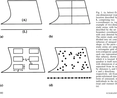
Fig. 1. (a, below) Example of one-dimensional transect with location described by the set
L, comprising two x-coordinates; (a, top) example of two-dimensional study arena, with location described by the set of (x, y) boundary coordinatesA, and with area denoted by A. (b) The entire study arena is divided into six contiguous subareas of unequal size and shape. (c) Six parts of the study arena are sampled with a rectangular grid of non-contiguous quadrats, each one representative of that subarea, shown in (b), in which it is located. Each quadrat is itself rectangular, with dimensions d and w, and separated from its neighbour by distances ldand lw, in the x and y directions,
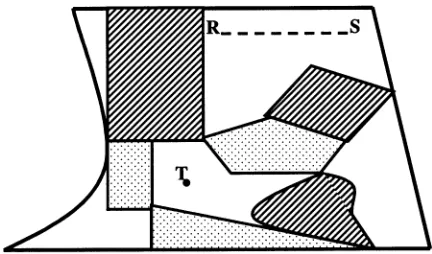
Fig. 2. Example of area-referenced geographic data, used typ-ically in landscape ecology. The study arena of Fig. 1a has been partitioned into areas, each with one of three attributes, denoted by the shading. Areas may be polygonal or irregularly shaped with curved boundaries. Also represented are a linear feature, denoted RS, and a point, denoted T.
let, Thiessen or Voronoi (see Dale 1999: Fig. 1.4 for an example). A closely related technique is the Delaunay triangulation. These techniques leave the (x,y) coordi-nates of the data unchanged. They effectively create additional, derived, area-referenced data, similar to that described in section 2) below.
Point-referenced (x, y) data may be amalgamated into a single value, to represent a subarea. This results in partial loss of spatial information, since the original locations can no longer be recovered. The resulting derived data are still explicitly spatial and retain the form (x%,y%), but x% and y% must now be defined, for example as the centroids of the subareas, used to trans-form the (x,y) data of Fig. 1d to the (x%,y%, z%) data type in Fig. 3c. In this example, a value of z%for each subarea has been derived from the count of the number of individuals within it. Comparing the two figures shows that almost all the information concerning clus-tering has been removed from the derived data. For transformations of (x,y,z) data, amalgamation of the z variable may also be achieved in very many ways, such as the mean magnitude of the z attribute, where the averaging is over the individuals located within each subarea.
Sampled data from quadrats is always derived, by definition, since all the data recorded from within the quadrat are somehow aggregated, to yield a single representative value. Usually, the derived (x%,y%) com-ponent representing the location of each quadrat is defined as its centroid, as in Fig. 3d, where the z’ value for each of the quadrats in Fig. 1c has been derived from the count of the number of individuals contained within it. Observe how much variability is induced into For any spatial data type, further information may
be available for each individual, through the recording of an extra attribute(s), z; such data are denoted (x,z) or (x, y, z). Attributes may have different forms, of which the simplest is a categorical quantal variable (male or female, dead or alive, Fig. 3a). Another form of z attribute might be an ordered categorical qualita-tive variable, such as a life-stage. Alternaqualita-tively, it could be a quantitative variable, such as the magnitude of an innoculum (Fig. 3b).
Many forms of data may be derived. One transfor-mation frequently applied to two-dimensional point-ref-erenced ecological data divides up the study arena according to the locations of individuals, into a mean-ingful tessellation of polygons, often named for
Dirich-Fig. 3. Further examples of forms of point-referenced data. The censussed mapped individuals of Fig. 1d, (a) with additional quantal attribute; (b) with additional continuous attribute with magnitude indicated by size of symbol; (c) as counts within each of the six contiguous dashed subareas of Fig. 1b; (d) as counts sampled by the six dashed non-contiguous quadrats of Fig. 1c.
the counts of Fig. 3d by the sampling process, com-pared with the censussed values shown in Fig. 3c; whatever loss of information is involved in derived censussed data, the loss from sampled data will be greater. Also, note the difference between recording a z attribute(s) on exhaustively censussed point-referenced individuals, and taking a point sample of an attribute that is a continuously distributed variable over the study arena, such as elevation. Both may involve irreg-ularly-spaced data of the form (x,y,z), but the latter has the properties of a sample, with the concomitant features of uncertainty and the intention to represent some larger unknown population.
Area-referenced data are common in landscape ecol-ogy and geography. All of the variations of point-refer-enced data discussed above apply equally to the area-referenced data exemplified in Fig. 2. This type is commonly represented either by a vector form, (A,z), where location coordinates defining each (possibly ir-regular) area are associated with attribute(s), or by a raster form, where locations are addressed by a grid of Cartesian coordinates and attributes pertain to a cell of fixed area at that location. Note that raster data can be stored as point-referenced data (x, y, z) but must include the crucial information of grid cell size; this representation is substantially equivalent to point-refer-enced data in subareas, where the loss of information is small and offset by a very large number of subareas.
In geography, a dichotomy is recognized between so-called ‘‘object’’ and ‘‘field’’ data models (Peuquet 1984, Gustafson 1998, Peuquet et al. 1999). The object model considers two-dimensional arenas populated by discrete entities whereas underlying the field model are variables assumed to vary continuously on a surface. Area-referenced data can be considered as either; within Geographic Information Systems software (Burrough and McDonnell 1998) (A,z) data are often represented as polygonal.
Sometimes, explicit spatial information might not exist, or if the data for analysis is recycled from previ-ous results, the information may have been degraded and lack the detail of the original records. Some meth-ods of data recording or amalgamation remove all explicit spatial information. For example, a common and powerful entity in spatial pattern analysis is termed a nearest neighbour (NN) distance (Donnelly 1978, Diggle 1983, Ripley 1988), defined for each censussed individual as the distance to its nearest neighbour. Hence, in the (x,y) data shown in Fig. 1d above, the individual labelled P has the individual labelled Q as its nearest neighbour and the distance PQ would be the NN distance associated with P. As can be seen, the relationship is not necessarily commutative, since the nearest neighbour of Q is not P. The set of NN distances for all individuals is not spatially-referenced, so is denoted by (z). However, it contains much implicit information concerning location, and may be used to
test for spatial randomness. A further example is the frequency distribution of counts in subareas or samples (e.g. the setz={3, 4, 6, 7, 7, 9} from Fig. 3c), stripped of its (x, y) coordinate information. From these six counts may be derived associated statistics such as the sample mean, sample variance, and quantities such as the variance to mean ratio, known as the index of dispersion (Fisher et al. 1922), I, which in this case is exactly 4. Note how I fails to capture any of the pattern in the original Fig. 1d.
Data taxonomy
Other proposals for data taxonomy have been made; some are not helpful because they are specific to disci-plines tangential to mainstream ecology (e.g. Gustafson 1998). Cressie’s (1991) taxonomy is not recommended because it makes insufficient distinction between the information available and the collection methods used to record it, particularly to reflect the effect of sam-pling. Also, it formally defines lattice data as encom-passing a finite, countable set of spatial locations, while confusingly exemplifying it by reference to remote sens-ing and medical image data that are both spatially continuous in nature. Additionally, it would benefit from a revision to link the term ‘‘geostatistical’’ with models or methods for spatial analysis, rather than with types of data.
Techniques for spatial analysis
Characteristics of spatial pattern
Fig. 4. Point locations of 32 individuals: (a) aggregated into 8 clusters, each with a random number of individuals, and centred on random locations; (b) arranged regularly; (c) that display spatial anisotropy; (d) that display non-stationary spatial structure, with half of the individuals aggregated into four clusters towards the top and left of the study arena and the other half, in the bottom-right of the area, arranged randomly. Note that in d the intensity of the process is roughly equal in the two parts of the area. In both a and b, one of the points has been labelled A and two circles, radii t1and t2, are shown centred on A.
corresponding multiplicity of mechanisms that generate them. Most methods identify particular characteristics of pattern, ranging from generic statistical measures, such as coefficient of variation among samples, to more specialized methods that address explicit ecological questions, such as indices of landscape habitat patch shape. Occasionally, methods such as geostatistics have arisen in one discipline and proved so useful that they have been embraced by mainstream ecology (Rossi et al. 1992, Liebhold et al. 1993). We focus on twelve methods, exemplified in analyses of the case studies. Some methods, such as fractal analysis (Stoyan and Stoyan 1994) or spectral methods (Mugglestone and Renshaw 1996), are omitted due to constraints of space. Detailed descriptions of methods may be found in cited sources or in the companion paper of Dale et al. (2002). Most methods seek to compare some feature of the spatial process ‘‘here’’ (at some local reference point), with the same feature ‘‘elsewhere’’, i.e. in another loca-tion(s). The reference point could be a randomly chosen location or individual. The feature described might be a count of a defined set of other individuals; or an
attribute, for example the volume of some organism; or a derived value, such as local density. The other loca-tion(s) may be a particular distance away in some given direction; or defined by a given interval centred on the reference point; or the next contiguous area in a se-quence; or the nth nearest individual. The definition ‘‘local’’ may shift, systematically or randomly, to en-compass different parts of the study arena, in turn.
Methods vary in the degree of information they impart. The simplest methods are descriptive displays of spatial information, consistent with Chatfield’s (1985) principles of initial data analysis. We stress the utility of mapping and simple summary statistics as a first step in the analysis of spatial data (Korie et al. 1998), and advocate the work of Tufte (1997) and Carr (1999) as an innovative source of ideas for visual pre-sentation. More sophisticated methods allow inference in the form of a test of the null hypothesis, sometimes more complex than that of complete spatial random-ness. Yet further information is offered by methods that estimate quantities. Finally, there are methods that fit spatial models, if enough data are available (Keitt et al. 2002).
Many ecological data sets exhibit different spatial pattern when viewed at one spatial extent than at another, a ‘‘scale’’ effect. For example, the point loca-tions in Fig. 4a are aggregated into clusters at small spatial extents, although the clusters themselves have a random number of individuals and random locations. Certain methods are designed specifically to study the relationship between the degree of pattern and its scale (Table 1), and see Dungan et al. (2002).
Another common spatial characteristic of ecological data is anisotropy, where the pattern itself changes with direction. In Fig. 4c the clusters are elongate in a specific direction and tend to be associated with each other more strongly in that direction. Compare Fig. 4a, where the pattern is random with respect to direction. Whereas global methods summarize patterns over the full extent of the area studied, in recent years there has been interest to develop methods that identify local variation (Anselin 1995, Getis and Ord 1995, Ord and Getis 1995, Sokal et al. 1998a, b) in spatial characteris-tics, such as aggregation, within the sampling domain (Table 1). Local methods such as wavelets and SADIE can be used to map and detect locations within the study arena that may drive the overall pattern, or which are outliers. When the underlying process that generates pattern varies across different regions within the area studied, a stationary model will not be appropriate. In Fig. 4d, although the intensity of the point process is roughly equal in the two parts of the area, individuals are aggregated in one part and randomly distributed in another. Many methods are based, to a small or large degree, on stationarity assumptions.
Methods appropriate for different data types
Point-referenced data,(x,y)
Questions asked of such data normally concern the spatial pattern of the individuals: are they clustered (as in Figs 1d, top and 4a) or regularly spaced (as in Figs 1d, below and 4b), or do they occur at random loca-tions? Ripley (1977, 1988) derived a method based on the indices, K. (t) and L.(t), scaled for intensity, that averages the number of individuals within a distance t of a randomly chosen individual. For an individual in an aggregated pattern, for example point A in Fig. 4a, the expected number of individuals within a circle of radius t1 that approximates to the dimensions of a typical cluster will be relatively large compared to the same number of individuals distributed randomly within the study arena. As the radius of the circle is gradually increased, say to t2, the area encompassed extends outside the cluster to which A belongs, but not yet into other clusters, so there are few extra individuals counted. This characteristic increase in the count over particular small intervals of t provides a signature to graphs of L.(t) vs t, that may be formally tested by
comparison with corresponding graphs generated by Monte Carlo simulation (Diggle 1983) for random pat-terns. Note that for a regular pattern, as in Fig. 4b, the reverse is the case: the count is fewer than expected for t1and greater for t2. Methods for this data type must allow for edge effects (Ripley 1988, Haase 1995).
Point-referenced data with attributes,(x,y,z)
Typical questions for such data are: is the apparent segregation in Fig. 3a of the solid from the open symbols real, and vice versa? Is the infection measured by the quantitative degree of innoculum shown in Fig. 3b dispersing from a point source, and if so, can we confirm that the source is located close to the centre of the study arena? With such a continuous attribute it is often of interest to determine whether its values are more similar than expected to those nearby, or more formally whether there exists detectable spatial autocor-relation, and if so, what is its relationship with the distance between points? When there are several z attributes, we are usually interested to know whether the variables are positively spatially associated (Perry 1998b, Liebhold and Sharov 1998) with each other or negatively spatially associated (termed ‘‘dissociated’’), once any induced (dis)similarity due to their individual spatial structure is allowed for (Clifford et al. 1989, Bocard et al. 1992, Dutilleul 1993). Alternatively, do they occur randomly with respect to one another?
Some methods that involvez-attributes are restricted to regularly spaced (x) or (x,y) data on a grid (Table 1). For example, ‘‘quadrat variance methods’’ (Dale 1999) which include ‘‘two-term local quadrat variance’’ (TTLQV) as well as 3TLQV and others, are used predominantly for one-dimensional regularly-spaced transect data. Second-order comparisons are made be-tween blocks of a given length, say d, of contiguous quadrats, through computation of their variance. Ag-glomeration into blocks using increasing values of d, within a hierarchy, allows plots of variance against d. Since the blocks are contiguous, block size is identical to the distance between block centres. The idea is that a peak in variance on this graph will indicate maximum contrast between patch and gap, if there is a stationary process with constant cluster size, at a distance equiva-lent to approximate cluster size. This allows the detec-tion, and in some cases the testing for significance of spatial pattern along the transect. Their analogues in two-dimensions include the block quadrat variance methods for (x%,y%,z%) data wherez%is a count, derived for insects by Bliss (1941), rediscovered for plants by Greig-Smith (1952) and later modifications such as 4TLQV (Dale 1999).
ECOGRAPHY
25:5
(2002)
585
Table 1. Description of methods for analysis of spatial data.
Allows
Type of data Original use Model Info. available Info. available 1- or 2-
Irregularly-Method Info. available
dimensions?
on anisotropy? spaced units
hypothesis on local
based? at multiple
pattern? allowed?
scales? tests?
possible no both yes
yes yes
Ripley’s K and L, etc. point-referenced plant ecology no locations, (x, y)
Quadrat variance methods point-referenced plant ecology no rarely yes no no 1 no locations, (x, z)
(TTLQV, etc.)
no rarely yes possible no 2 no
plant ecology point-referenced
Block quadrat variance
locations with methods (Greig-Smith,
attributes, (x, y, z) 4TLQV, etc.)
point-referenced no yes yes yes no both yes
Correlograms (Moran’s I, geography Geary’s c, etc.) locations with
attributes, (x, y, z)
yes no both yes
Geostatistics (variograms), (x, y, z) Earth sciences no no yes PQV
no both yes
yes yes
Geostatistics (kriging) (x, y, z) Earth sciences yes yes
Angular correlation (x, y, z) geography no yes no yes no 2 yes
yes no yes both no
Wavelets (x, y, z) statistics no no
no no yes both yes
SADIE (x, y, z) insect ecology no yes
rarely no rarely no 2
rarely yes
landscape ecology area-referenced
Landscape ecology metrics
locations with (edge density, shape
indices, etc.) attributes, (A, z)
no yes no no no both
applied yes
Variance-mean methods non-spatially
entomology referenced data,
(Morisita, Taylor, etc.)
attributes only, (z)
yes no no no both yes
plant ecology and
Nearest neighbour methods (z) no
particular distance, d, and the relationship between variance (or semi-variance) and d is graphed and stud-ied, thereby quantifying structure at multiple spatial extents. Some of these methods, Moran’s I (Moran 1950) and Geary’s c, allow significance tests of com-plete spatial randomness (Cliff and Ord 1973, 1981, Sokal and Oden 1978, Oden 1984). Geostatistical meth-ods in this class include the variogram, correlogram, and covariance function. We include paired quadrat variance (PQV) in this section because, although strictly a quadrat variance method, the size of its block never varies; indeed, despite their independent development, the variogram and PQV are mathematically identical and thus provide the same information (ver Hoef et al. 1993, Dale and Mah 1998, Dale et al. 2002). Geostatis-tical methods are not generally used for hypothesis testing, but their associated models of spatial depen-dence are used for spatial interpolation, modelling and simulation (Isaaks and Srivastava 1989, Rossi et al. 1992). The idea underlying all the methods is that spatial autocorrelation declines, and therefore variance increases, with increasing d, until some maximum vari-ance, termed the ‘‘sill’’, is reached, at a value of d termed the ‘‘range’’. The range is an estimate of average patch and gap size. For very small d the variance, termed the ‘‘nugget’’, although a minimum, may still be non-zero; it is equated to measurement error plus the variance at smaller unit sizes. Whenzis a dummy (0, 1) variable, measuring presence, some methods in this section (such as indicator variograms) are effectively utilizing (x,y) data.
Many methods have been adapted for the study of anisotropy (Oden and Sokal 1986, Isaaks and Srivas-tava 1989, Falsetti and Sokal 1993) and local informa-tion (Anselin 1995, Getis and Ord 1995, Ord and Getis 1995, Sokal et al. 1998a, b). Specific methods (Table 1) to detect anisotropy include Rosenberg (2000) and an angular method using spatial correlation, derived by Simon (1997). The latter projects each (x, y, z) point onto an axis in a test direction, say u, then calculates the correlation, r, between the positions of the projected points along thisu-axis and the z-attribute. The values of (u, r) are then plotted in polar coordinates; a bulge in the resulting curve indicates the direction of greatest change in z.
Wavelet analysis may also be used to quantify spatial pattern over a variety of spatial extents, usually for one-dimensional data. It has much in common with the methods described above, albeit based on a different statistical approach (Bradshaw and Spies 1992, Dale and Mah 1998). The emphasis is on the ‘‘decomposi-tion’’ of the data into repeating patterns that are com-pared with the wavelet function’s shape over varying window-widths, which are equivalent to distance lags. In this there are similarities to the quadrat variance methods (Dale et al. 2002), but wavelets allow contrasts of a specific and more complex functional form, using
shapes such as the ‘‘Mexican hat’’ (Dale 1999). A powerful feature of this method is the lack of any stationarity assumption.
SADIE is a class of methods designed to detect spatial pattern in the form of clusters, either of patches or gaps (Perry et al. 1999). The calculations (Dale et al. 2002) also involve comparisons of local density with those elsewhere, but made across the whole study arena simultaneously. Each sample unit is ascribed an index of clustering, and the overall degree of clustering into patches and gaps is assessed by a randomization test. A specific extension to spatial association (Winder et al. 2001) is made by comparing the clustering indices of two sets of data across the sample units. A local index of association,xk, may be derived at each sample unit, k, and these may be combined to give an overall value, X. The power of these methods comes from the ability to describe and map local variation of spatial pattern and association.
Area-referenced data(A), (A,z)
Data that are area-referenced are common in landscape ecology, particularly in polygonal form. The methodol-ogy for their analysis has not advanced as fast as other techniques described here. Only few involve inferential tests; they are largely descriptive. As for point data, one option is to sample by overlaying a grid and convert to (x, y, z) spatially-referenced attribute data (see above and Discussion). However, if the degree of fragmenta-tion is of particular interest then methods such as those described in Turner and Gardner (1991) and McGarigal and Marks (1995) may be applied to polygonal data in either raster or vector form. Patch size and its coeffi-cient of variation (CV) are examples of the numerous indices; there is no space here for an exhaustive list. The latter is a measure of landscape fragmentation and heterogeneity but with important limitations (McGari-gal and Marks 1995). Edge density (Morgan and Gates 1982), defined as a measure of edge length standardized by enclosed area, is positively related to the degree of fragmentation of the habitat, but also to its shape. For regular shapes it is minimum for a circle, and maximal for a linear feature. Total edge length is the sum of all lengths of edges of patches of one landscape type. Mean shape index, the ratio of perimeter to area, is a measure of shape complexity; it approaches unity for perfect figures such as circles and increases with shape irregularity (McGarigal and Marks 1995). When sam-pling relatively small areas, the area-weighted shape index is considered more meaningful, because it gives greater weight to large polygons.
Attribute-only data(z)
neigh-bour, where p is usually unity. The set of distances is not spatially explicit, even though it is derived from point-referenced locations. Hypothesis tests (Clark and Evans 1954) are usually based on the expected distribu-tion of such distances for a random arrangement of individuals. Highly clustered patterns tend to have rela-tively small (e.g. Fig. 4a), and regular patterns (e.g. Fig. 4b) relatively large NN distances, respectively. They are similar to methods like Ripley’s L.(t) function in that they must be adjusted to allow for edge effects, but differ from them in that they utilize less spatial infor-mation and cannot identify pattern at multiple spatial extents.
Early studies of spatial pattern such as Bliss (1941) were based on summary statistics from frequency distri-butions (David and Moore 1954), and used little or no spatially-explicit data. Techniques relied on the fact that samples of randomly arranged individuals would yield counts that followed the Poisson distribution, but an observed Poisson distribution does not necessarily imply randomness (Hurlbert 1990). Indeed, the set of counts: {0, 0, 1, 1, 2, 2, 2, 2, 3, 3, 5}, conforms closely to a Poisson distribution, but if sampled in that order along a line transect shows an obvious linear trend departing strongly from randomness. Recent methods (Upton and Fingleton 1985, Perry and Woiwod 1992) include the index of dispersion I, Morista’s index, Lloyd’s (1967) index of mean crowding and Taylor’s power law (Taylor et al. 1978), used extensively in animal ecology. Jumars et al. (1977) and Perry (1998a) have cautioned users to distinguish non-randomness in the form of statistical variance-heterogeneity from true spatial non-randomness. The only valid spatial infer-ence possible to make from an observation of variance-heterogeneity is that there must be spatial pattern for some unknown support smaller than that used to derive the observed counts.
Origins of methods
While it can be shown that many of the methods described above are computationally similar (Dale et al. 2002), it is worth noting that many differences among the methods can be attributed to their historical devel-opment in different disciplines (Table 1). In applied entomology, limited computational resources before 1970 precluded the widespread development of methods that utilized specific spatial coordinates, although the SADIE method now exists to address this issue. Later, methods developed for plant ecology were applied to two-dimensional coordinate locations of individuals, but often lacked a tractable underlying statistical model. Geostatistical methods were developed for prob-lems in the applied Earth sciences and emphasized estimation rather than the detection of spatial pattern by hypothesis testing. However, their development from
an underlying generic statistical model has made these methods useful for purposes of spatial interpolation and simulation, and they are applied increasingly to ecological problems (Rossi et al. 1992, Liebhold et al. 1993).
Case studies
Four case studies are used to illustrate the application of the methods outlined above to the data types dis-cussed above. These exemplify comparisons between methods, regarding their applicability to answer partic-ular questions, their ability to provide different types of information and to allow contrasting inferences.
Case study 1: counts of three shrub species along a transect
The data (Dale and Zbigniewicz 1997) are censussed percentage cover of each of six boreal shrub species, of which only three are considered here. They are, in order of abundance, Betula glandulosa, Salix glauca, and Picea glauca, measured between 1 and 3 m height. Cover was measured, along a linear transect of 1001 contiguous quadrats, each 0.1 m2, in shrub-dominated vegetation. Separate measurements were done for each species; the combined total for more than one species may be \100%. All three species were most abundant towards the left end of the transect and all were absent in \60% of quadrats. Questions Dale and Zbigniewicz posed included: is there pattern of plants within species? What is the average patch- and gap-size? Is there spatial association between species? The (x, y, z) data are analyzed as collected: derived total cover per contigu-ous quadrat.
Betula glandulosa
The observed, raw data exhibited numerous, relatively small patches (Fig. 5). Initial inspection of presence-absence revealed 80 runs of quadrats that contained some Betula glandulosa, with mean length 0.48 m, separated by 80 runs that contained none, with a much greater mean length of 0.77 m. Indeed, for such sparse data, with \60% zero cover, there must be large differences between patch and gap size.
The analysis begins with various approaches to esti-mate a dominant cluster size. Because of the large number of quadrats, the variogram (Fig. 6) was smooth and the lack of a nugget effect emphasized that most of the fine spatial structure was captured. A spherical model was appropriate and the range of ca 0.7 m implied a relatively small dominant cluster size.
The PQV plot, identical to the variogram except that it was plotted over a greater distance on the x-axis,
Fig. 5. Percent cover of Betula glandulosa. One quadrat is equivalent to 0.1 m.
The Mexican-Hat wavelet analysis (Fig. 7) showed by the intense yellow shading at small window-widths and by the marginal mean graph, that the greatest contrasts within windows occur at relatively small window widths of 10 quadrats, the estimated dominant cluster size. The spike of largest variance, occurring around quadrat 277, successfully identified the longest run of substan-tial cover, ten successive quadrats each of at least 90%. Another region in which the wavelet analysis identified large variance was the broad peak around quadrat 660; there, B. glandulosa was present in 34 successive quadrats, but with considerable variability in cover from quadrat to quadrat.
Moran’s I was highly significant overall. At the shortest distances, I declined with increasing lag, until at a distance of 0.7 m spatial autocorrelation became negative; this was interpreted as an estimate of the dominant cluster size. At larger lag distances I had relatively small values. The strongly negative autocorre-lations at lags 7.5 and 80 m were difficult to relate to the data and could not readily be interpreted.
The SADIE analysis showed very strong clustering. The mean patch and gap clustering indices were 3.12 (pB0.0005) and −3.30 (pB0.0005), respectively. Just over one-third of the total length of the transect had no detectable pattern (white areas, Fig. 8); these areas were spread fairly evenly. The size of the 73 patches ranged from 0.1 to 1.7 m (mean 0.40 m, SEM 0.046 m, median 0.2 m), and of the 106 gaps from 0.1 to 3.3 m (mean 0.30 m, SEM 0.031 m, median 0.2 m). The SADIE clusters relate to spatial pattern rather than abundance per se, and so the large proportion of the transect where there was no pattern broke up the runs of less-abundant quadrats into the relatively large number of gap clusters.
Of the methods studied, the variogram/PQV and Moran’s I matched each other closely and gave sensible estimates of dominant cluster size, averaged of necessity over patches and gaps. The Mexican-Hat wavelet Fig. 6. Variogram ofBetula glandulosadata in Fig. 5.
Semi-variance, gamma, is plotted against distance in metres.
added no useful information for these data; there was no evidence of damped periodicity beyond the esti-mated range. The TTLQV and 3TLQV plots were similar. The 3TLQV plot, using more data, had three peaks: one from ca 1.7 to 2.5 m, another from 4 to 7 m, and a third from 13 to 17 m. It was unclear to what features of the data the larger peaks corresponded.
Fig. 8. SADIE analysis of Betula glandulosa. Red shading indicates patches with cluster index values \1.5; blue shading indicates gaps with index values B−1.5; white areas represent lengths that are neither patches nor gaps.
provided a larger estimate, but gave very useful insights into other aspects of the data. TTLQV and 3TLQV performed poorly, and added no extra useful interpre-tation. The SADIE method provided separate and dif-ferent estimates of patch and gap size, which were sensible.
Picea glauca
The observedPicea glaucadata exhibited a small num-ber of relatively small patches (Fig. 9a), having similar structure to the Betula data above, but of a much sparser nature. There were 20 small bursts of cover, ranging from 0.1 to 1 m with mean length 0.24 m. Less than 5% of quadrats were occupied and the runs con-taining noPicearanged up to 18.1 m with mean length 4.54 m.
The PQV (Fig. 10, top) implied an average cluster size of 1.1 m, although for situations where the ob-served patch and gap size are as disparate as here this has little interpretive utility. Its interesting feature was a sudden decline in variance at around 10.5 m, unusual for a PQV/variogram, and caused by the sparseness of the data. This distance was highlighted because it repre-sented roughly the minimum between any of the four patches containing at least one quadrat with \80% cover shown in Fig. 9a. At shorter distances, variance was dominated by the comparison between those pairs of quadrats, one of which contained a member of one of these four patches and the other of which did not. The upward slope over long stretches of the plot indi-cated the clear trend in the data. The TTLQV and 3TLQV plots showed no sudden decline in variance;
they indicated structure with an average cluster size ca 6 m and ca 3.8 m, respectively.
Marginal variance in the Mexican-Hat wavelet plot mirrored the positions of the four largest patches re-ferred to above, but showed little further structure; marginal variance was maximal at 0.9 m.
Usually, Geary’s c and Moran’s I (Fig. 10, middle and below) are very similar except for inversion, but for these data they differed. Both indicated an dominant average cluster size of 0.9 m, but whereas I remained fairly flat thereafter, c continued to increase before crossing the x-axis again around 10.5 m, informatively indicating a second scale of pattern at the same distance as found by PQV (Fig. 10, top).
The SADIE analysis confirmed substantial spatial pattern, the mean clustering indices for patches being 3.25 (pB0.0013) and for gaps −3.88 (pB0.0013). A proportion of 0.29 of the total length of the transect had no detectable pattern, almost all within the left-hand half of the transect. The 19 patches were correctly identified, ranging in size from 0.1 to 0.5 m (mean 0.18 m, SEM 0.031 m, median 0.1 m), and the 43 gaps from 0.1 to 12.7 m (mean 1.6 m, SEM 0.36 m, median 0.8 m).
Salix glauca
Data forSalix glauca was similar in structure to both other species. There was considerable spatial pattern, with a degree of sparseness midway between the other two species (Fig. 9b). No feature of any analyses was fundamentally different from those discussed above, so none is reported, but the data are presented to inform
Fig. 9. Percent cover of (a) Picea glaucaand (b)Salix glauca. One quadrat is equivalent to 0.1 m.
Fig. 10. Methods that measure variability plotted against varying extents in units of metres (ten quadrats) for Picea glauca. Above is local paired quadrat variance, PQV; under-neath are two correlograms, Moran’s I (middle graph) and Geary’s c (lower graph). Filled symbols indicate significant individual lags (pB0.05).
Cross-correlograms and cross-variograms also revealed little structure.
However, SADIE analysis of the cluster indices re-vealed strongly significant positive association between the spatial pattern in pairs of all three species (Betula glandulosaandPicea glauca, X=0.244, pB0.001; Be -tula glandulosa andSalix glauca, X=0.133, p=0.001; Picea glauca and Salix glauca, X=0.401, pB0.001). The method of Clifford et al. (1989) suggested an approximate halving of the effective degrees of freedom for each species pair; probability levels and confidence limits, from randomizations under the null hypothesis of no association, were adjusted accordingly. In a map of local association, xk, for Picea glauca and Salix glauca (Fig. 11), the dominance of plum shading over green demonstrates an overall positive association be-tween the species. The positions of the shaded contours distinguishes areas in which relatively large local values occurred. For example, the plum shading between quadrats 333 and 336 reflects values of positive local association, arising from the coincidence of patches exceeding 40% cover for both species. Detrending the cluster indices by a quadratic function suggested that the association found was due mainly to larger-scale similarities between the species. All maps showed con-siderable clustering of local association towards the extreme right of the transect, where the coincidences of several gaps reflected long runs of quadrats where cover was exceedingly sparse or absent for all species.
The difference between the results for the simple correlation analyses and SADIE arise, as for the single species comparisons, because the former makes com-parisons between variables that are abundance/density estimates, where an isolated large value contributes equally to the computed statistic as does a similar value in a patch. By contrast, the SADIE analysis is based upon the degree of spatial pattern, so isolated values are deliberately downweighted.
the analysis of relationships between the species, dis-cussed below.
Relationships between the species
Using the raw cover data, correlations between species pairs were small (Betula glandulosa and Picea glauca, r=0.0188; Betula glandulosa and Salix glauca, r= −0.0577; Picea glauca and Salix glauca, r=0.0016). None was significant, before or after accounting for spatial structure using the Clifford et al. (1989) method.
Fig. 12. (a) Locations of the 4357Ambrosia dumosaindividuals in the 100×100 m study arena. (b) Frequency
distribution of the count of individuals per 5×5 m subarea quadrat.
Case study 2: mapped locations and volume of a desert shrub
The data (Miriti et al. 1998) are the locations and logarithmically-transformed estimated plant canopy volumes of all individual adults of the deciduous desert shrubAmbrosia dumosa, recorded on a single occasion in a 100×100 m area in the Colorado Desert (Wright and Howe 1987). These data form a subset of a larger and phased study of plant dynamics with different life stages, in whichAmbrosia dumosaencompassed almost two-thirds of all recorded stems. The study site was selected deliberately to minimize heterogeneity at-tributable to environmental variation. Miriti et al. (1998), and see references within) were interested in the relative importance and effects of possible intra-specific interference and negative plant-to-plant interactions on spatial distribution, and to quantify the spatial scales
over which major processes operated. Here, four ver-sions of the data were analyzed: (x,y) point locations, derived (x,y,z) counts in 5×5 m contiguous subareas, (z) attributes (nearest neighbour distances and vol-umes), and derived (x,y,z) mean volume per plant in 5×5 m contiguous subareas.
Individuals of A. dumosa seemed to be distributed throughout the study arena with considerable, but small-scale aggregation (Fig. 12a). Two or three bands of relatively low or zero density, of width ca 15 m, appeared to run roughly north-west to south-east across the area. The frequency distribution of counts per 5×5 m quadrat shows a typically right-skewed distribution with a mean of 10.86 plants per quadrat and a similar mode (Fig. 12b); the variance/mean ratio was 4.3, which indicates significant numerical variance heterogeneity.
Fig. 13. Ripley’s L.(t) function forAmbrosia dumosa individuals, where t represents the radius in metres of the notional circle drawn around a randomly chosen plant. Also shown are upper, Ru(t) and lower, Rl(t) envelopes representing upper 97.5%-iles and lower 2.5%-iles under the null hypothesis of complete spatial randomness, derived from Monte Carlo randomizations. Here, for visual clarity, the three y-variables are each transformed by subtracting t, prior to plotting: L.(t) – t are filled circles, Ru(t) – t are open triangles, Rl(t) – t are open diamonds. The x-axis represents t. Filled circles above the upper envelope indicate significant aggregation and those below the lower envelope indicate significant regularity.
Fig. 14. Semivariance from directional variograms for Am -brosia dumosa counts, in 5×5 m quadrats, plotted against distance in metres, in directions: 0°, 45°, 90° and 135°.
as data the counts of individuals within contiguous 2n m2square subareas, where n=2, 3, and upwards. This gave an initial, rough indication of the relationship of how aggregation varied with subarea size. It showed moderate and non-significant heterogeneity, but which crucially decreased monotonically with subarea from the smallest, with side 2 m, and became virtually indis-tinguishable from random at the largest tested, with side 11.3 m. Hence, both these results confirmed the conclusions of Miriti et al. (1998) and the visual impres-sion from Fig. 12a. There was considerable aggregation at the smallest spatial extents, consistent with some unspecified plant-to-plant interactions, but this seemed to decrease over medium extents of ca 100 m2with sides of 10 m, a distance beyond which an individual plant would expect to exert an influence over others.
To quantify further the relationship between aggrega-tion and spatial scale of distance, t, we plotted Ripley’s L.(t) function versus t for the (x,y) point location data (Fig. 13). This confirmed one indication from the blocked quadrat variance analysis, that there was sig-nificant and strong aggregation from the smallest scale studied, a distance of 0.7 m, which declined almost monotonically with t. However, this did not cross the upper envelope until ca 24 m. Unusually, L.(t) contin-ued to decline, indicating regularity by falling substan-tially below the lower envelope, and not until 60 m did Previous analyses by Miriti et al. (1998) showed that
the total nearest neighbour distance was 386.0, which exceeded the expectation for a random distribution, using Donnelly’s (1978) method, by over 15 times the standard deviation, indicating highly significant aggre-gation. They also used a hierarchical blocked quadrat variance method (Dale 1999), based on Morisita’s (1959) index (the test for which is equivalent to Greig-Smith’s (1952) test of the index of dispersion I), using
Fig. 16. Frequency distribution ofAmbrosia dumosa logarith-mically-transformed plant canopy volume per plant.
ensures that there is considerable autocorrelation in the plot of L.(t) vs t. Hence, it would not only be unwise to infer that true regularity existed at the scale of 60 m, but also to infer that the distance at which the spatial process became random was 24 m, or indeed to attempt a precise estimate of this distance. In summary, the most important information conveyed by this analysis relates to the existence of the strongest pattern at the smallest distances.
The following analyses were done for the counts of individuals in 5×5 m contiguous subareas. Directional variograms were calculated (Fig. 14). The large nugget variance and shallow slope up to the sill supported the conclusion above, that the major structure in the data occurred at distances smaller than were resolvable by the subarea size. The variogram range also confirmed the indication, from L.(t), that there was some larger-scale structure up to distances of ca 25 m. This distance was confirmed by the results from both Moran’s I and Geary’s c. Additionally, the variograms showed some mild anisotropy in the 135° direction for distances \40 m, providing further support for the existence of the bands referred to above, although no directionality was detected by an angular correlation analysis.
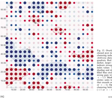
The SADIE analysis confirmed the presence of large-scale patches of varying size up to ca 400 m2 (mean patch cluster index=1.29; p=0.025), and gaps (mean gap cluster index= −1.35; p=0.048). The most nota-ble feature was a long gap ca 10 m wide stretching from left to right across almost the entire width of the hectare block (Fig. 15), and supporting further the existence of the bands of low density.
it increase again relative to the randomizations. This is not thought to reflect an important facet of the data. It was probably a manifestation of the change in intensity along the diagonal that runs from lower-left to upper-right of the area, which appears to cycle 2.5 times as it traverses the two large relatively empty bands referred to above. The wavelength of this cycle is ca (402) m=57 m which coincides well with the value of t for which L.(t) is a minimum. The abundance of individuals
Fig. 17. (a) The 100×100 grid of NDVI derived from AVHRR data from 7 to 20 August, 1992, collected over the Cascade Mountains. Darker shades represent smaller values. (b) The 100×100 grid of elevation data from the same location. (c) Frequency distribution of NDVI and (d) elevation in feet.
Fig. 18. (a) Moran’s I correlogram for NDVI; all lags are significant (pB0.05). (b) Angular correlation for NDVI. (c) Directional variogram for NDVI and (d) elevation.
There was a very strong linear relationship between logarithmically-transformed plant canopy volume and counts, and when mapped these two derived (z) vari-ables appeared very similar. However, a frequency dis-tribution of transformed volume per plant (Fig. 16) showed a clearly bimodal distribution with relatively many plants in the smallest size class and a second more symmetric mode for much larger plants. Such bimodality is characteristic of many long-lived plants in which seeds readily germinate, but mortality of smaller individuals is high until a certain size threshold is reached, after which survival probabilities increase until senescence. Also, mapping revealed considerable spatial pattern in the values of volume per plant within the 5×5 m contiguous subareas. Broadly, volumes per plant were greater in the left-hand half of the study arena (xB50, mean transformed volume per plant=
12.93 with SEM 0.121; x\50, mean transformed vol-ume per plant=12.42 with SEM 0.099). Clustering was significant (SADIE indices both p=0.0002), with two regions of relatively low volume per plant (top centre and lower-right side, each 200 – 300 m2) and one 200 m2 patch of greater than average volume, at the lower-left of the area. The reason for spatial structure in these growth differences between plants is unknown.
Case study 3: remotely-sensed AVHRR data in the Cascade Mountains
Since 1982, the Advanced Very High-Resolution Ra-diometer (AVHRR) satellite imager (Eidenshink 1992) has collected image data from daily coverage of the Earth, using a nominal 1-km sampling rate. We down-loaded archived and processed area-referenced AVHRR data, collected from 7 to 20 August 1992, from the EROS Data Center web site http://
edcwww.cr.usgs.gov/landdaac/1KM/comp10d.html.
NDVI data and resampled to the same 1×1 km grid cells (Fig. 17b). Frequency distributions for NDVI (Fig. 17c) and elevation (measured in feet, Fig. 17d) exhib-ited only slight skewness and no transformation was needed before analysis. Specific questions posed for these data were: what are the spatial patterns of NDVI and elevation and how similar are they? Are these two variables correlated?
Declining values in Moran’s I correlogram (Fig. 18a) and increasing values in the directional variogram (Fig. 18c) indicated strong, positive autocorrelation in vege-tation across the map, while their monotonic nature across the full range of distances indicated the presence of a large-scale trend or gradient of vegetation. This trend was present in every direction except for a 45° angle. The angular correlation diagram (Fig. 18b) con-firmed this directionality, achieving maximal values be-tween 90° and 135°. This revealed anisotropy may be seen clearly in the raw data (Fig. 17a); highest NDVI values are to the north-west and lowest values to the south-east. This pattern probably reflects the distribu-tion of forested areas along the eastern slope of the North Cascade Mountains. Forests are more abundant at higher elevations and high desert vegetation is domi-nant at the lower elevations to the south-west. The correlogram, angular correlation diagram and an-isotropy directions for elevation were so similar to those for NDVI that they are not shown. The direc-tional variogram for elevation (Fig. 18d) confirms the anisotropy shown by the trend and direction of the strongest gradient evident in the map (Fig. 17b).
Rossi et al. (1992) pointed out that a large-scale trend, such as the anisotropy found here for NDVI and elevation, could obscure patterns of spatial dependence at smaller lag distances. Here, it is unclear from the directional variograms (Fig. 18c, d) whether anisotropy
exists in autocorrelation at short lag distances or is limited to the large-scale trend.
In order to investigate further the scale of autocorre-lation and anisotropy, we removed the large-scale trend in both data sets by fitting a model of the form: zx,y=a+b1x+b2y. Estimates of the parameters for NDVI were: a= −172.4, b1= −0.000173, b2= 0.000107; and for elevation: a= −55119, b1=
−0.0303, b2=0.0258. The directional variograms for the detrended NDVI residuals from this model (Fig. 19a) differed from those discussed above; they reached a maximum (sill), and indicated less anisotropy, al-though the range appeared slightly longer in the 135° direction than for other angles. The directional vari-ograms of the detrended elevation data (Fig. 19b) showed precisely the same differences, but additionally, for the 90° angle the elevation variogram exhibited a slight ‘‘hole effect’’, first increasing then decreasing with increasing lag distances. This pattern is characteristic of some sort of oscillatory undulation or repetitive fluctu-ation (Isaaks and Srivastava 1989) here probably caused by the regular alternation of valleys and ridges. The same pattern also appears, although less distinctly, in the 90° variogram (Fig. 19a) of the NDVI data.
Overall, there was a striking similarity between the NDVI and elevation variograms. Both had nugget ef-fects near zero for the raw data, indicating the existence of a very continuous, smooth surface. The ranges of both detrended sets of data were between 10 000 and 20 000 m, presumably reflecting the average distance between mountain peaks. However, the similarity of the variograms cannot be used alone to infer their associa-tion, since many different spatial arrangements may share the same variogram (Liebhold and Sharov 1998). We calculated a Pearson correlation coefficient of 0.4916 between raw NDVI and elevation; a ‘‘naı¨ve’’ test
Fig. 19. Directional variograms of detrended data. (a) NDVI, (b) elevation.
Fig. 20. Vector representation of land use and land cover (LULC) data.
for association without adjusting for spatial autocor-relation would indicate significance (pB0.0001). However, the existence of autocorrelation in both variables violates the assumption of independence among samples and the test of correlation requires adjustment (Clifford et al. 1989, Bocard et al. 1992, Dutilleul 1993). This is because the presence of spatial autocorrelation indicates that the amount of informa-tion in a set of data is less, and may be considerably less, than that in a sample of the same size where there is none. This loss of information is therefore allowed for by an adjustment that leaves the magni-tude of the correlation unchanged, but alters the de-grees of freedom of the test. We used the variograms in Fig. 18 to adjust the degrees of freedom from 9998 to 14.52 using the method of Clifford et al. (1989); the revised, valid test was not significant (p=0.0679). Hence, the observed large magnitude of the correla-tion was almost completely due to common and large-scale spatial structure; after adjustment for this effect, correlation was only marginally significant.
Case study 4: land cover in Monterey County, California
Land use land cover (LULC) data are area-referenced data developed by the US Geological Survey (USGS) for every portion of the conterminous USA at either a 1:100 000 or 1:250 000 scale. They are available from the USGS web site in either vector or raster format (Anon. 1986). Data are derived by manual interpretation of aerial photographs, incorporating in-formation from earlier land-use maps and field sur-veys. Land-use cover is classified according to the scheme developed by Anderson et al. (1976).
The data used in this case study consisted of the south-eastern corner of the 1:100 000 Monterey quad-rangle located in the central coast region of Califor-nia. The study arena spanned 30.4 km from east to
west and 27.2 km from south to north. Only land areas classified into three land cover classes were in-cluded: herbaceous rangeland (code 31); shrub and brush rangeland (code 32); and mixed rangeland (code 33). All analyses were performed on data pro-jected to the Universal Transverse Mercator projec-tion (zone=10) (Fig. 20). The analysis described here is limited to those descriptive statistics (McGarigal and Marks 1995) that measure patch size, edge den-sity and shape from polygonal data (Table 2). Mixed rangeland was the dominant land cover type and also had the greatest mean patch size. Both fragmentary indices, patch size CV and edge density, were also largest for mixed rangeland. Also, both the mean shape index and the area-weighted shape index were greatest for the mixed rangeland cover type, indicat-ing a greater complexity of polygon shape.
Directional variograms for shrub rangeland (Fig. 21b) demonstrated anisotropy; the range was consider-ably longer in the north and northwest directions. This difference appeared to reflect both an elongation of patches in a consistent north-westerly direction, as well as the arrangement of patches along a band running in that same direction (Fig. 20). This anisotropy probably reflects ridge topography that may be associated with vegetation. The hole effect (depression at ca 2300 m) in the north-east directional variogram (Fig. 21b) reflected the alternating presence and absence encountered when traversing the study arena in a direction perpendicular to the angle of patch elongation (Fig. 20).
Discussion
We have attempted to offer, for a limited number of sets of data, some flavour of the kinds of outputs, inferences and interpretations possible from spatial analysis. Readers must realize that we have not at-tempted an exhaustive account. Many methods are capable of extension to provide further features, to meet specific needs. For example, almost all of the local quadrat variance methods detect the average size of patches and gaps in a phased pattern along a transect, but new local variance (Galiano 1982) detects the size of the smallest phase of the pattern, whether it be patches or gaps. This, when combined with other local quadrat variance methods, allows separate estimation of patch and gap size.
We give only four recommendations to ecologists with spatial data in search of methods with which to analyze them. First, make extensive use of simple visu-alization techniques such as graphs and mapping (Tufte 1997, Carr 1999) as a first step to understanding spatial characteristics in the data. Second, select statistical methods that are available and appropriate for the data type. Third, select a method that can answer pertinent questions and provide relevant spatial information. Reference to Table 1 may help the selection process. Given the suitability of several methods, it would be invidious and naı¨ve to attempt to go beyond this to recommend which single specific technique to use. Readers must form their own conclusions, informed by the theoretical properties of the methods and their performance in the above case studies. Most methods are distinct and no single one can identify all of the spatial characteristics in data. Therefore, our fourth recommendation is to employ several different tech-niques. We do not believe that any methods we have examined intrinsically provide redundant information, fail to detect real patterns, or identify patterns that are not real.
In certain circumstances, it may be sensible to widen the possible range of techniques that may be brought to bear on a problem, by converting between data types.
ECOGRAPHY 25:5 (2002) 597