Security Analysis on Network Systems Based on Some Stochastic Models

University of New Orleans University of New Orleans

ScholarWorks@UNO

ScholarWorks@UNO

University of New Orleans Theses and

Dissertations Dissertations and Theses

Fall 12-2014

Security Analysis on Network Systems Based on Some Stochastic

Security Analysis on Network Systems Based on Some Stochastic

Models

Models

Xiaohu Li [email protected]

Follow this and additional works at: https://scholarworks.uno.edu/td

Part of the Applied Statistics Commons, Industrial Engineering Commons, Probability Commons, Risk Analysis Commons, and the Systems Engineering Commons

Recommended Citation Recommended Citation

Li, Xiaohu, "Security Analysis on Network Systems Based on Some Stochastic Models" (2014). University of New Orleans Theses and Dissertations. 1931.

https://scholarworks.uno.edu/td/1931

Security Analysis on Network Systems

Based on Some Stochastic Models

A Dissertation

Submitted to the Graduate Faculty of the University of New Orleans

in partial fulfillment of the requirements for the degree of

Doctor of Engineering and Applied Science in

Mathematics

by

Xiaohu Li

Ph.D. University of New Orleans, 2014

Acknowledgments

I would like to give my sincere gratitude toward Professor Linxiong Li, who generously

spent numerous afternoons in the past two years on discussing lots of details in this

dissertation. Professor Li also read through the earlier draft of this dissertation with

great patience and presented many valuable suggestions, without which, I believe, there

is still a long way for it to take the present form. As a respectable professor, Dr. Li taught

me quite a lot in statistical science; As a faith-worthy friend, Dr. Li also helped me to

deal with other things in my campus life.

I would like to thank other four committee members,

Professor Tumulesh Solanky Department of Mathematics, College of Sciences, Uni-versity of New Orleans

Professor Jairo Santanilla Department of Mathematics, College of Sciences, Univer-sity of New Orleans

Professor Xiaorong Li Department of Electrical Engineering, College of Engineering, University of New Orleans

Associate Professor Nikolas I. Xiros Department of Naval Architecture and Marine Engineering, College of Engineering, University of New Orleans

I would like to extend my thank to those faculties who brought me into the world of

statistics and engineering through teaching the interesting graduate courses. Besides, I

want to address the gratitude to several of graduate students in China, their studious

effort to pursue academic excellence is always the main driving force of my research work

in reliability, security and risk management.

Finally, I am deeply grateful to my wife, Xiao Zhou, for her continuous support, kind

assistance and great patience and to my brother and sisters for taking care of my parents

in the past two decades. I dedicate this dissertation to my parents.

Xiaohu Li

Department of Mathematics

University of New Orleans

New Orleans LA 70148

Contents

Abstract viii

1 Introduction and Preliminaries 1

1.1 Introduction . . . 1

1.1.1 Peer to peer network . . . 2

1.1.2 Vulnerable network . . . 4

1.2 Preliminaries . . . 8

1.2.1 Important notations . . . 8

1.2.2 Several aging properties . . . 8

1.2.3 Some stochastic orders . . . 9

1.2.4 The k-out-of-n structure . . . 11

1.3 Archimedean copula . . . 12

1.4 Summary . . . 14

2 Resilience Analysis of P2P Network Systems 15 2.1 Introduction . . . 15

2.2 Model description . . . 16

2.3 Resilience analysis . . . 19

2.4 Reliability analysis . . . 24

2.4.2 Stochastic monotonicity . . . 26

2.5 Interdependence among users lifetimes . . . 27

2.6 Identifying the NWUE order . . . 29

2.6.1 Graphical method based on TTT plot . . . 30

2.6.2 A nonparametric test . . . 35

2.6.3 Concluding remarks . . . 39

3 Security Analysis of Compromised-Neighbor-Tolerant Networks 41 3.1 Introduction . . . 41

3.2 The model . . . 43

3.3 Main analytical results . . . 47

3.3.1 Equation of the probability to be compromised . . . 47

3.3.2 Impact of topology on vulnerability graph . . . 51

3.4 Probability bounds . . . 57

3.5 Concluding remarks and future work . . . 64

A R codes 66 A.1 Codes to produce TTT plot in Figure 2.4 . . . 66

A.2 Codes to produce TTT plot in Figure 2.5 . . . 67

B Mathematica codes 69 B.1 Codes to plot upper/lower bounds in Figure 3.2 . . . 69

B.2 Codes to plot lower bounds in Figure 3.2 . . . 70

B.3 Codes to plot upper bounds in Figure 3.3 . . . 70

Bibliography 79

List of Figures

1.1 A server based network . . . 3

1.2 A P2P based network . . . 3

1.3 A depiction of a vulnerable network with security components . . . 5

1.4 A depiction of a vulnerable network with security components . . . 7

2.1 A typical depiction of a node with 3-out-of-6 structure . . . 17

2.2 Pr(U2:3 ≤t ) −Pr(V2:3 ≤t ) . . . 30

2.3 Scaled TTT plots of Pareto distributions withα= 100, 5, 2, 1.25 . . . 31

2.4 TTT plots of air-conditioning systems in airplane: 8045 (◦), 7909 (•) . . . 32

2.5 TTT plots of network chatting systems: Yahoo (◦), Skype (•) . . . 34

3.1 A depiction of the evolving process of a vulnerable network . . . 44

3.2 Upper bound (top) and lower bound (bottom) by (3.5) . . . 62

List of Tables

2.1 Life times of air-conditioning systems of planes . . . 32

2.2 Times user spend in chatting systems . . . 34

2.3 Statistics on data sets of air-conditioning and network chatting systems . . . 39

Abstract

Due to great effort from mathematicians, physicists and computer scientists, network

science has attained rapid development during the past decades. However, because of the

complexity, most researches in this area are conducted only based upon experiments and

simulations, it is critical to do research based on theoretical results so as to gain more

insight on how the structure of a network affects the security. This dissertation introduces

some stochastic and statistical models on certain networks and uses a k-out-of-n tolerant

structure to characterize both logically and physically the behavior of nodes. Based upon

these models, we draw several illuminating results in the following two aspects, which are

consistent with what computer scientists have observed in either practical situations or

experimental studies.

Suppose that the node in a P2P network loses the designed function or service when

some of its neighbors are disconnected. By studying the isolation probability and the

durable time of a single user, we prove that the network with the user’s lifetime having

more NWUE-ness is more resilient in the sense of having a smaller probability to be

iso-lated by neighbors and longer time to be online without being interrupted. Meanwhile,

some preservation properties are also studied for the durable time of a network.

Addition-ally, in order to apply the model in practice, both graphical and nonparametric statistical

methods are developed and are employed to a real data set.

network systems based on their vulnerability graph abstractions. A node loses its designed

function when certain number of its neighbors arecompromised in the sense of being taken over by the malicious codes or the hacker. The attack compromises some nodes, and the

victimized nodes become accomplices. We derived an equation to solve the probability

for a node to be compromised in a network. Since this equation has no explicit solution,

we also established new lower and upper bounds for the probability.

The two models proposed herewith generalize existing models in the literature, the

corresponding theoretical results effectively improve those known results and hence carry

an insight on designing a more secure system and enhancing the security of an existing

system.

Key words: Durable time; Exponential distribution; Harmonic mean; Increasing convex order;

Isolation probability; Jackknifing;

k-out-of-n; NWUE;

Pareto distribution; Power law distribution;

Stochastic orders; Random graph;

TTT plot; U-statistic

1

Introduction and Preliminaries

1.1 Introduction

Computer and network security has become a rather popular and important topic in

the past two decades. A simple Google search based on the keyword “computer and

network security” showed 27.8 million items on September 25, 2014. In general, network

security mainly aims to protect the entire infrastructure of a network system as well

as its corresponding services from unauthorized access. There are several fundamental

components in network security:

(i) Security-specific infrastructures, such as hardware- and software-based fire-walls and

physical security approaches;

(ii) Security polices, which include security protocols, users authentications,

authoriza-tions, access controls, information integrity and confidentiality;

(iii) Detection of malicious programs, including anti-viruses, worms, or Trojan horses,

and spyware or malware;

(iv) Intrusion detection and prevention, which encompasses network traffic surveillance

Since the topic of network security links a great number of research areas and

disci-plines, we will investigate the role the infrastructures of a network plays in the system’s

security based upon some stochastic models. For an overall introduction on network

se-curity, including key tools and technologies used to secure network access, please refer to

Malik (2003) and Laet and Schauwers (2005).

1.1.1

Peer to peer network

As a decentralized structure, a Peer-to-Peer (P2P) computer network utilizes diverse

connectivity among users participating a network and the cumulative bandwidth of them

rather than conventional centralized resources where a relatively low number of servers

play the key role in providing a service or application.

P2P networks, which are usually used for connecting nodes through largely ad hoc

connections, are useful for many purposes. Sharing content files containing audio, video,

data or anything in digital format and real time data. P2P networks can be classified by

what they can be used for: (i) file sharing, (ii) telephony, (iii) media streaming (audio,

video), and (iv) discussion forums etc.

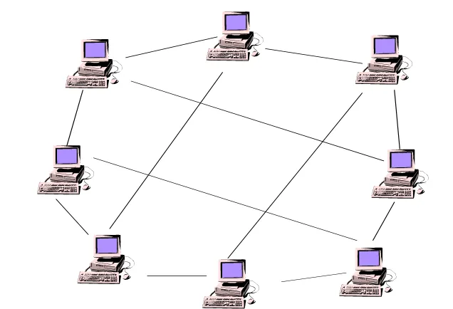
A pure P2P network does not have any clients or servers but only equal peer nodes

that function as both “clients” and “servers” simultaneously to the other nodes in the

network (see Figure 1.1.1). This structure of network differs from the client-server model

where communication is mostly between the node and a central server (see Figure 1.1.1).

As a typical example, an FTP server transfers file in a manner totally different from

that a P2P network does. Actually, the client and server programs in an FTP server are

quite distinct, the clients initiate the download/uploads, and the servers offer the service

according to these requests.

Besides the pure P2P network, there are quite a lot of Hybrid P2P networks. For

Figure 1.1: A server based network

a client-server form. To disseminate Usenet news articles over the entire Usenet network,

news servers communicated with each other. However, the news server system acts in

a client-server style when individual users access a local news server to deal with news.

As another example, in an SMTP email system, the core email relaying network of mail

transfer agents from a P2P model while the periphery of Mail user agents and their

direct connections is client-server. On the other hand, some other networks, for example,

Napster, OpenNAP and IRC, use a client-server structure for some tasks (e.g. searching)

and a P2P structure for others.

Currently, P2P structure rapidly evolves and is widely used in distributed networks

not only computer to computer but also human to human. Without any server, a node in

P2P network mainly relies upon connections from its neighbors to operate correctly and

losing some connections implies the failure of this node, it is very important to study its

resilience and reliability. Leonard et al (2007) built the lifetime model for a P2P network,

it is assumed that the node is isolated when it is physically disconnected from all its

neighbors, that is, all connections are broken. In Chapter 2, we study the resilience of

the pure P2P network through a new lifetime model, which is a generalization of that

proposed by Leonard et al (2007) in the sense that a node loses the function and service

if and only if some of its neighbor nodes are disconnected, this enable the new model

to include both physical and logical isolation and hence to be more useful in practical

situations. We derive the probability for a node to be isolated and the expected dural

time, and show that the more heavier the tail of probability of the lifetime is, the more

resilient the P2P network is.

1.1.2

Vulnerable network

With the rapid development of computer, this world gets more involved into networks.

network and hence result in hazardous loss in business. In fact, the past two decades

witnessed numerous such kind of cases. This fundamentally attributes to vulnerability of

networks and it is rather urgent to study the network security so as to effectively defense

the network from being invaded.

Network security usually consists of those provisions made in an underlying computer

network topology, policies adopted by the network administrator to protect the network,

the network-accessible resources from unauthorized access, and consistent and continuous

monitoring to measure its effectiveness.

Figure 1.3: A depiction of a vulnerable network with security components

Network security originates from authenticating all user a username and a password.

After the authentication, a fire wall is employed to enforce access policies which control

from being accessed without being authorized, however, this component fails to check

potentially harmful contents such as computer worms and virus being disseminated over

the network. In order to screen these malicious codes, an intrusion prevention system

(IPS) (see Mirkovic et al, 2004) is designed to detect and prevent such malware from

invading the network. Additionally, IPS also monitors for suspicious network traffic for

contents, volume and anomalies so as to protect the network from being attacked by

denial of service. On the other hand, to keep privacy, communication between two host

nodes in the network is encrypted as well. Meanwhile, all individual events occurred in the

network are tracked and audited for a later high level analysis. Besides, as surveillance and

early-warning tools, Honeypots (see Grimes, R. A., 2005) essentially decoying

network-accessible resources is also deployed in a network. Techniques employed by attackers

attempting to compromise any decoy resources are studied during and after an attack to

keep an eye on those new exploitation techniques. Such analysis could be used to further

tighten security of the actual network being protected by the honey pot.

For a comprehensive summary of standard concepts and methods in network security,

please refer to Curtin (1997) and Simmonds et al (2004), which presents all notions and

techniques in the form of an extensible ontology of network security attacks.

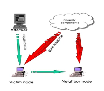
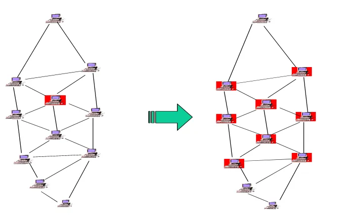
In Chapter 3, the network is abstracted as a vulnerable graph, which is composed

of nodes (users) and edges (connections). In order to model the infrastructure of the

network, a node of the graph is always assumed to have a random degree representing its

neighbors. Since our aim is to investigate how the random degree has an impact on the

network security, an attack outside the network is supposed to attempt to compromise

nodes all the time and any compromised nodes become his accomplices in the sense

of having the capability of compromising their neighbors. On the other hand, due to

these security components deployed over the network, the attacker only penetrates the

after being compromised and hence become secure after being disinfected. Likewise, to

make our model more multifunctional, it is also assumed that a node is compromised only

when at lease some prefixed number of neighbors are infected. This model is an substantial

extension of that studied by Li et al (2011). In effect, we proved that the probability for a

node to be compromised is increasing as the random degree grows in the increasing convex

order. Among others, new lower and upper bounds are also built for the probability to

be compromised, evaluations reveals that they are better than those developed in Li et

al (2011). The main result shows that power law graph is more vulnerable than both the

random graph and the regular graph.

1.2 Preliminaries

For ease of references, let us recall some fundamental yet important concepts on aging

property and stochastic ordering, which will be employed to characterize network systems

in the following chapters.

Throughout this dissertation, the term increasing is used instead of monotone non-decreasing and the term decreasing is used instead of monotone non-increasing. We also assume that all random variables under consideration have 0 as the common left end

point of their supports, and all random variables are implicitly assumed to be absolutely

continuous.

1.2.1

Important notations

1.2.2

Several aging properties

For a nonnegative random variable X with distribution function F and the reliability

function ¯F = 1−F, let

Xt =X−t|X > t

be the residual lifetime of X at time t≥0, the mean residual lifetime

µF(t) = E[X−t|X > t] =

∫ _∞

t

¯ F(x) dx ¯

F(t) .

Definition 1.2.1 A random lifetime X is said to be of

(i) increasing failure rate (IFR) if the cumulative failure rate −ln ¯F(t) is convex with respect tot ≥0;

star-shaped with respect to t≥0, that is, −1_tlog ¯F(t) is increasing int ≥0;

(iii) decreasing mean residual life (DMRL) if µF(s)≥µF(t) for all t≥s≥0;

(iv) new better than used in expectation (NBUE) if µF(t)≤µF(0) for all t≥0.

Reversing the monotone property and the inequality above, we get their dual versions:

DFR (decreasing failure rate), DFRA (decreasing failure rate in average), IMRL

(increas-ing mean residual life) and NWUE (new better than used in expectation). The follow(increas-ing

chain of implications is well-known,

IF R(DF R) =⇒IF RA(DF RA) =⇒DM RL(IM RL) =⇒N BU E(N W U E).

For more details on these nonparametric aging properties, please refer Barlow and

Proschan (1981), Lai and Xie (2006).

1.2.3

Some stochastic orders

For two nonnegative random variableX andY with distribution functionsF and G, and

reliability function ¯F = 1−F and ¯G = 1−G, denote F−1 _{and G}−1 _{the corresponding}

right continuous inverses ofF and G respectively.

Definition 1.2.2 X is said to be smaller than Y in the

(i) hazard rate order (denoted byX ≤hr Y) if ¯F(t)/G(t) is decreasing in¯ t ≥0;

(ii) stochastic order(denoted as X ≤st Y) if Pr(X > t)≤Pr(Y > t) for allt;

(iii) increasing convex order (denoted as X ≤icx Y) if

∫ _∞

t

Pr(X > x) dx≤ ∫ _∞

t

(iv) harmonic mean residual life order (denoted by X ≤hmrl Y) if, for all t ≥0, [ 1 t ∫ t 0 1 µF(u)

du ]−1

≤ [ 1 t ∫ t 0 1 µG(u)

du ]−1

,

for which the expectations exist.

(v) convex order (denoted by X ≤cx Y) if E[ϕ(X)]≤E[ϕ(Y)] for any convex ϕ.

It holds evidently that

X ≤hrY =⇒X ≤st Y =⇒X ≤icx Y =⇒X≤cx Y.

Kochar and Wiens (1987) proposed a partial order to compare the NBUE-ness of two

life distributions. Since NBUE and NWUE are dual with each other, for convenience, we

call it the NWUE order.

Definition 1.2.3 X is said to be more NWUE than Y (denoted byX ≥nwue Y) if

µF

(

F−1(v)) µG

(

G−1_(v)) ≥

µF

µG

, for all v ∈(0,1). (1.1)

As a function of v ∈(0,1),

∫ F−1_(v)

0

¯ F(t) dt

is the well-known total time on test (TTT) transform of the distribution F of a random lifetime X. The scaled TTT transform

φ−_F1(v) = 1 µF

∫ F−1_(v)

0

¯ F(t) dt

plays an important role in characterizing aging property of random lifetime. One may see

Recently, Kochar et al. (2002) proposed a new partial order: X is said to be larger

than Y in the total time on test transformorder (denoted by X ≤tttY) if

∫ F−1_(v)

0

¯

F(x) dx≥

∫ G−1_(v)

0

¯

G(x) dx, for all v ∈(0,1).

These two stochastic orders mentioned above have a close relation in the sense that when

E[X] =E[Y], X ≥nwueY is equivalent to X ≥ttt Y.

Readers may refer to M¨uller and Stoyan (2002), Shaked and Shanthikumar (2007),

and Li and Li (2013) for more details on these stochastic orders.

1.2.4

The

k

-out-of-

n

structure

Let X1, X2,· · ·, Xn denote n independent component lifetimes with Xi,n being the i-th

order statistic, here i = 1,· · · , n. A k-out-of-n system of these components functions if

and only if at leastkcomponents function. Whenk =n, the system has a series structure

with lifetime

Xn,n = min{X1,· · · , Xn};

whereas for k = 1, it reduces to a parallel structure with lifetime

X1,n = max{X1,· · · , Xn}.

Thus, ak-out-of-n system is more general than either a series or a parallel structure. The

lifetime of this system is simply given by the order statistic Xn−k+1:n.

As a fault-tolerant structure, the k-out-of-n system is widely used in many

practi-cal situations, including, for example, electronic engineering, manufacturing and defense

industry etc. One may refer to Kuo and Zuo (2006) and Lai and Xie (2006) for

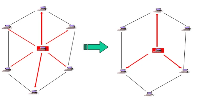
to describe a network which is tolerant to some compromised neighbors due to anti-virus

software.

1.3 Archimedean copula

Mutual independence among multiple random variables is common in reliability and risk

management. The interdependence among components’ lifetimes, random risks, and

po-tential loss/returns etc. cannot be ignored in practical situations. In classical statistical

theory, Pearson’s correlation coefficient is usually utilized to measure the dependence

among random variables. In Chapter 2 we will instead employ copula, a functional

mea-sure, to characterize the association among network users’ lifetimes.

For a random vector X = (X1, . . . , Xn) with joint distribution function F, survival

function ¯F and univariate marginal distribution functionsF1, . . . , Fn, itscopula is defined

as

CX(u1,· · · , un) = F

(

F₁−1(u1),· · · , Fn−1(un)

)

, 0< u1,· · ·, un <1.

In parallel, thesurvival copula is b

CX(u1,· · · , un) = ¯F

(_¯

F₁−1(u1),· · · ,F¯n−1(un)

)

, 0< u1,· · ·, un <1.

Since the copula does not contain any information of marginal distributions, it provides

us with a rather convenient way to impose a dependence structure onto predetermined

marginal distributions in practice. Actually a large number of excellent applications

of copulas can be found in various areas, and so far copula has become more or less

a standard tool in risk management, finance, econometrics and actuarial science etc.

Recently, Copulas are being used for reliability analysis of complex systems of machine

and Hong (2003), and copula functions have been successfully applied to the database

formulation for the reliability analysis of highway bridges, and to various multivariate

simulation studies in civil, mechanical and offshore engineering, see for example Thompson

and Kilgore(2011). In literature on statistics, there are a large number of copulas depicting

various dependence structures, Hutchinson and Lai (1990) and Nelsen (2006) provide a

wide range families of bivariate copulas along with their properties. In the past twenty

years, Archimedean copulas became particularly popular because of its mathematical

tractability and the capability of capturing wide ranges of dependence. Notably, since

the statistical inference on Archimedean copulas has got well developed in this decade,

excellent applications are coming to the fore in various areas.

Definition 1.3.1 (McNeil and Ne˘slehov´a (2009)) For a non-increasing and contin-uous function ϕ : [0,+∞) 7→ [0,1] such that ϕ(0) = 1 and ϕ(+∞) = 0, let ψ = ϕ−1 _be

the pseudo-inverse,

Cϕ(u1,· · · , un) =ϕ

(

ψ(u1) +· · ·+ψ(un)

)

, for (u1,· · · , un)∈[0,1]n, (1.2)

is called anArchimedean copulawith the generatorϕif (−1)k_ϕ(k)_(x)≥_{0 fork= 0, . . . , n}−

2 and (−1)n−2ϕ(n−2)(x) is non-increasing and convex.

The generatorϕis said to be strict ifϕ(+∞) = 0. As is well-known, the Archimedean family contains a plenty of useful copulas, including some well-known ones. For example,

the independence (product) copula C1(u) =

∏n

i=1ui with the generator ϕ(t) = e−t, the

Clayton copula

C2(u) =

(∏n

i=1

with the generator ϕ(t) = (θt+ 1)−1/θ _{for θ}≥_{0, and the Ali-Mikhail-Haq (AMH) copula}

C3(u) =

(1−θ)

n

∏

i=1

ui

n

∏

i=1

(1−θ+θui)−θ n

∏

i=1

ui

.

with the generator ϕ(t) = _e1t−₋θ_θ for θ∈[0,1). For more on copula and its applications, we

refer readers to Joe (1997) and Nelsen (2006).

1.4 Summary

Resilience analysis of P2P network

By studying the isolation probability and the durable time of a single user, we conduct

resilience and reliability analysis of the P2P network, which is widely used in

commu-nication systems in recent several years due to the decentralized property. It is proved

that the network with the user’s lifetime having more NWUE-ness is more resilient. Both

graphical and nonparametric statistical methods are developed to test the NWUE order

between two real data sets.

Security analysis of networks

A stochastic model is introduced to investigate security of network systems based on

their vulnerability graph abstractions. Instead of doing traditional security analysis, we

employ the increasing convex ordering to study the underlying vulnerability graph, the

main theoretical results carry an insight on designing a more secure system and enhancing

2

Resilience Analysis of P2P Network

Systems

2.1 Introduction

Peer-to-Peer (P2P) internet network allows a group of computer users equipped with the

same networking program to connect with each other for the purpose of directly accessing

files from one another’s hard drives. A P2P network functions by connecting individual

computers together to share files instead of going through a central server. P2P networks

can be classified by what they can be used for, for instance, content delivery, file sharing,

telephony, media streaming (audio, video) and discussion forums etc. In the current study

of P2P networks, Kaashoek and Karger (2003) and Stoica et al. (2001) investigate the

single-node isolation, Aspnes et al. (2002), Ganesh and Massoulie (2003), Gummadi et al.

(2003), and Massouli´e (2003) etc discuss the disconnection of the entire graph. Bhagwan

et al. (2003) is among the first to pay attention to the more realistic P2P failure models, in

which the intrinsic behavior of internet users is taken into account and the departments

of users depend on more complex factors including their attention span and browsing

habits, and so on, other than the traditional simple binary metric. In order to investigate

model based on users’ lifetimes and studies the stochastic resilience of P2P networks, in

which an user stays online for random periods of time till all his neighbors go off line or

he leaves the network on his own initiative. In this model, the random lifetime that an

arriving user will stay on line reflects both the behavior of the user itself and the duration

of its service to the entire P2P network community.

This chapter proposes a more general P2P network model, in which an user is isolated

only when a number of its neighbors leave the network and hence the P2P model in

Leonard et al. (2005) is included as a special case. We further investigate both the

stochastic resilience and reliability properties of this new model. It is proved that the

network with the user’s lifetime having more NWUE-ness is more resilient. The rest

of this paper is organized as below: Section 2 introduces the new P2P network model.

Section 3 studies the stochastic resilience by using the isolation probability of a single

user, and Section 4 discusses some reliability properties of the available time of a single

user in the network. Finally, both graphical and nonparametric methods are developed

in section 5 to detect the NWUE order between two data sets. All main conclusions are

consistent with those obtained through experiments in the literature.

2.2 Model description

In this section, we describe our P2P network model in details and present its rationality.

For an internet user, let X, a nonnegative random variable, be the lifetime that stays

online in the network for his own purpose or providing services to other peers. Saroiu et al.

(2002), Bustemante and Qiao (2003) pointed out that the distribution of an user’s lifetime

in practical P2P network very well accords with Pareto distribution, which possesses of

the well-known new worse than used in expectation (NWUE) property (they called it the

found that the distribution of the lifetime of an UNIX process is also Pareto, it was named

there as used better than new in expectation(UBNE) instead of NWUE. Here, we assume a general type of the distribution of the user’s lifetime other than Pareto law so that the

new model not only is suitable for human-based P2P networks but also can be applied to

non-human network systems.

For a new internet user with random lifetime X having the distribution function F,

assume

Figure 2.1: A typical depiction of a node with 3-out-of-6 structure

(i) the P2P network system has operated so long that there is no transient effect, that

is, the expected lifetime of the new user is negligible in contrast to the age of the

whole P2P system;

(ii) when entering the system, the new user randomly (in the sense that each existing

user has the same probability to be selected) picks k neighbors from the existing

nodes in the system as soon as it enters into the system;

(iii) the selection of neighbors is independent of both the lifetime X and the neighbors’

(iv) the time that a new user will spend in the system is independent of those of his

neighbors.

Since the P2P network has operated for a sufficiently long period when the new user

joins the system, it is reasonable to suppose that all those selected neighbors have ˜X, the

equilibrium renewal excess lifetime ofX, as their common residual lifetime, that is,

F_X˜(t) =

1 µF

∫ t

0

¯

F(x) dx,

where µF =E[X] and t≥0.

For 1 ≤ r ≤ k, denote ˜Xr the residual lifetime of the r-th neighbor. According to

David and Nagaraja (2003), the order statistic ˜Xr,k, which gives the residual lifetime of

the r-th failed neighbor, has the reliability function

¯

F_X˜_r,k(t) =

r−1

∑ i=0 ( k i )

[F_X˜(t)]i

[_¯ F_X˜(t)

]k−i

=r (

k r

) ∫ 1

F_X˜(t)

ur−1(1−u)k−rdu

and the probability density function

f_X˜_r,k(t) =

r µ ( k r ) ¯

F(t) [F_X˜(t)]r−1

[_¯ F_X˜(t)

]k−r

.

In the study of passive model in Leonard et al. (2005), a node is considered as isolated

after its last surviving neighbor fails. However, in many realistic environments, neighbors

of a node usually fail to service due to lower performance and in fact it reaches the isolation

state only if there are1 ≤ r ≤ k neighbors in failure. An instantiation of such a case is

that this node is sharing an animation file with its neighbors. Under the condition that

a fraction of its neighbors (not necessary all its neighbors) fail to service, the display of

the animation file is so incoherent that this node can be considered as disconnected. As

or disconnected only when more than r−1 neighbors fail to service. This is in fact the

famous r-out-of-k structure and thus the passive model in Leonard et al. (2005) is the

special case with r =k.

We will investigate the stochastic resilience of this P2P model by using the isolation probability

πr(X) = Pr

(

X >X˜r,k

)

, (2.1)

which denotes the probability that the new node outlives the residual lifetime of itsr-th

neighbor before it decides to leave the system. It is obvious that larger isolation probability

means worse resilience of the P2P network. On the other hand, we will employ

Tr(X) = min

{

X,X˜r,k

}

(2.2)

rather than ˜Xr,k to measure the durable time of a new node in a P2P network. It should

be marked here that Leonard et al. (2005) studies P2P networks by using ˜Xk,k, the time

that all k neighbors of the new node are simultaneously in failure state before it decides

to leave the system. However, as a competition between the lifetime X and the lifetime ˜

Xr,k, Tr(X) takes into account both the failure due to neighbors and that due to the new

user itself, it is more reasonable to serve as a metric to measure the stochastic resilience

of P2P networks.

2.3 Resilience analysis

Resilience analysis of random graphs and various types of deterministic networks has

attracted considerable interest of researchers during the past several decades. For more

details, please refer to Bollob´as (2001), Burtin (1977), and Leighton et al. (1995). Along

the network appears disconnection or demonstrates noticeably lower performance to its

users. Assuming uniformly random node failure, Stoica et al. (2001), Bollob´as (2001),

Gummadi et al. (2003) derive the conditions from different points of view under which

the networks stay connected after some nodes fail.

In this section, we study the resilience of P2P network systems by evaluating the

isolation probability for any given user. As described in Section 2, a node with lifetimeX

is forced to disconnect from the system only if X is greater than ˜Xr,k, 1≤ r≤k. Then,

the isolation probability is

πr(X) = Pr

(_˜

Xr,k< X

)

= ∫ _∞

0

Pr(X > t)f_X˜_r,k(x) dt

= r µk ( k r ) ∫ _∞ 0 ¯ F2(t)

(∫ t

0

¯ F(u) du

)r−1(∫ _∞

t

¯ F(u) du

)k−r

dt. (2.3)

As illustrations, isolation probabilities corresponding to the three popular lifetime

distributions are evaluated in the following examples.

Example 2.3.1 (Pareto distribution) Suppose the user has a lifetimeX with proba-bility distribution

G(x) = 1− (

1 + t β

)₋α

, t >0, α >1, β > 0.

Then, for any 1≤r ≤k, the isolation probability

πr(X) =r

( k r

) ( α−1

β

)k∫ _∞

0

( 1+t

β

)₋2α[∫ t

0 ( 1+u β )₋α du

]r−1[∫

∞ t ( 1+u β )₋α du ]k−r

dt = ( k r )

r(α−1) β

∫ _∞

0

( 1 + t

β

)₋2α[

1− (

1 + t β

)1−α]r−1(

1 + t β

)(1−α)(k−r)

= (

k r

)

r(α−1) β ∫ _∞ 0 [ 1− ( 1 + t

β

)1−α]r−1(

1 + t β

)(1−α)(k−r)−2α

dt

=r (

k r

) ∫ 1

0

tk−r+αα−1 (1−t)r−1dt (2.4)

= k! (k−r)!

Γ(k−r+ 1 + α α−1

)

Γ(k+ 1 + _αα₋₁) , for any 1≤r≤k.

Example 2.3.2 (Exponential distribution) Suppose the user has a lifetime Y with distribution

F(x) = 1−e−λt, t≥0.

According to (2.3), any new node has the isolation probability

πr(Y) = r

( k r ) λk ∫ _∞ 0

e−2λt λr−1

(

1−e−λt)r−1 1 λk−r

(

e−λt)k−r dt

= r ( k r ) λ ∫ _∞ 0 (

e−λt)k−r+2(1−e−λt)r−1 dt

= r (

k r

) ∫ 1

0

tk−r+1(1−t)r−1dt (2.5)

= k!

(r−1)!(k−r)!

(r−1)!(k−r+ 1)! (k+ 1)!

= k−r+ 1

k+ 1 , for any 1≤r≤k.

Example 2.3.3 (Uniform distribution) Suppose the userZ has a lifetime with uni-form distribution on the interval (0,2µ), that is, the distribution function

H(x) = t

Then, the isolation probability is

πr(Z) =

( k r ) r µk

∫ 2µ

0

( 1− t

2µ

)2[∫ t

0

( 1− u

2µ )

du ]r−1

· [∫ 2µ

t

( 1− u

2µ )

du ]k−r

dt = r µ ( k r

) ∫ 2µ

0

( 2µ−t

2µ )2[

1− (

2µ−t 2µ

)2]r−1(

2µ−x 2µ

)2(k−r)

dt

= r (

k r

) ∫ 1

0

tk−r+12(1−t)r−1dt (2.6)

= k! (k−r)!

Γ(k−r+3₂) Γ(k+3

2

) , for any 1≤r≤k.

From (2.4), (2.5) and (2.6), we observe the following:

(i) All of the three probabilities of isolation are independent of the expectation of

the user’s lifetime. So, it seems that property of the distribution instead of the

expectation has direct impact on the isolation probability.

(ii) The isolation probability corresponding to Pareto lifetime is the smallest one, the

uniform distribution achieves the largest isolation probability. Thus, we may

con-clude that the P2P network that users has Pareto lifetime is the most resilient one.

Based upon the above two facts, one may wonder whether the isolation probability

preserves some stochastic order on user’s lifetime, that is, πr(X) < πr(Y) holds for X

smaller than Y in some stochastic sense. As a positive answer, Theorem 2.3.4 below

asserts that a P2P network with users’ lifetime having a stronger NWUE property is

Theorem 2.3.4 Suppose that X and Y are two nonnegative random variables which represent user lifetimes of two different P2P systems, respectively. Then, X ≥nwue Y

implies πr(X)≤πr(Y).

Proof: For any 1 ≤r≤k, the isolation probability πr(X) can be rephrased as

πr(X) = Pr( ˜Xr,k< X)

= ∫ _∞

0

F_X˜_r,k(x) dF(x)

= r ( k r ) ∫ _∞ 0

∫ FX˜(x)

0

ur−1(1−u)k−rdudF(x)

= r (

k r

) ∫ φ−_F1(v)

0

ur−1(1−u)k−rdudF(x)

= r (

k r

) ∫ 1

0

∫ φ−_F1(v)

0

ur−1(1−u)k−rdudv,

here the scaled TTT transform

φ−_F1(v) = 1 µF

∫ F−1_(v)

0

¯ F(t) dt.

Likewise, the isolation probability

πr(Y) = r

( k r

) ∫ 1

0

∫ φ−_G1(v)

0

ur−1(1−u)k−rdudv.

Note thatX ≥nwue Y if and only if, for all v ∈(0,1),

1 µF

∫ F−1_(v)

0

¯

F(u) du≥ 1 µG

∫ G−1_(v)

0

¯

G(u) du,

the desired result follows immediately.

For the three distributions in Examples 2.3.2, 2.3.1 and 2.3.3, it is easy to verify that

As a result, it holds that X ≥nwue Y ≥nwue Z. According to Theorem 2.3.4, we have

πr(X)≤πr(Y)≤πr(Z), which can also be verified directly in Examples 2.3.1, 2.3.2 and

2.3.3.

2.4 Reliability analysis

The mean durable time of a user entering into a P2P network system is derived as below.

Proposition 2.4.1 For a P2P network system with user’s lifetime X,

E[Tr(X)] =

r µF

k+ 1, for all r= 1,· · · , k.

Proof: Since Tr(X) is nonnegative, it holds that

E[Tr(X)] =

∫ _∞

0

Pr(min{X,X˜r,k

}

> x)dx

= ∫ _∞

0

¯

F(x) ¯F_X˜_r,k(x) dx

= r ( k r ) ∫ _∞ 0 ¯ F(x) [∫ 1

FX˜(x)

ur−1(1−u)k−rdu ] dx = r ( k r

) ∫ 1

0

ur−1(1−u)k−r

[∫ F−_˜1

X (u)

0

¯ F(x) dx

] du = µr ( k r

) ∫ 1

0

ur−1(1−u)k−r

[∫ F−_˜1

X (u)

0

dF_X˜(x)

] du = µr ( k r

) ∫ 1

0

ur(1−u)k−rdu = r µF

k+ 1, for any 1≤r ≤k.

The above proposition reveals that the durable time of a new user in P2P network

distribution, the expected time it stays online depends upon the user’s lifetime distribution

only through its expectation.

2.4.1

Preservation of aging properties

The next result asserts that the durable time of the user in P2P system preserves both

IFR and IFRA properties of the user’s lifetime distribution.

Theorem 2.4.2 If X is IFR (IFRA), then Tr(X) is also IFR (IFRA).

Proof: IFR implies DMRL. It is known that the DMRL property of X is equivalent to the IFR property of ˜X. Since IFR property is preserved by thek-out-of-n structure with

i.i.d units, it follows that ˜Xr,k is IFR. On the other hand, IFR property is also preserved

by series system with independent components. So, we obtain the preservation of IFR.

Since IFRA property is preserved for coherent structure (see Barlow and Proschan

(1981)), the rest proof is the same as before.

As an application of Theorem 2.4.2, we build a lower bound of reliability of the durable

time of the user in P2P network.

Corollary 2.4.3 Let X be a nonnegative random variable which represents the user’s lifetime of P2P network system. If X is IFRA with mean µ, then, for all 1≤r≤k,

¯

FTr(X)(x)≥ (

1−(k+ 1)t rµ

)

+

, for all t≥0,

where x+= max{x,0}.

Proof: Theorem 2.4.2 guarantees that Tr(X) is IFRA and hence NBUE. By Hu et al

(2001), it holds that X is NBUE if and only if ˜X ≤st X, which implies

FTr(X)(x)≤

1

E[T (X)] ∫ t

¯

FTr(X)(u) du≤

for all 1≤r≤k and t≥0. This completes the proof.

2.4.2

Stochastic monotonicity

Hu et al. (2001) characterized some stochastic orders in terms of other stochastic orders

between their corresponding equilibrium versions. Especially, it is proved thatX ≤hr (≤st

)Y if and only if ˜X ≤hr (≤st) ˜Y. Based on this and the fact that both the order ≤hr and

the order ≤st are closed fork-out-of-n structure with independent units (see Shaked and

Shanthikumar (2007)), it is easy to obtain the proposition below, which asserts that the

durable time of the user in P2P network preserves both the hazard rate order and the

stochastic order of the parent distribution.

Proposition 2.4.4 If X ≤hr (≤st)Y, then Tr(X)≤hr (≤st)Tr(Y).

At the beginning of this section, we have concluded that the durable time of the

user in P2P network is distribution free. In other words, we cannot distinguish the

difference between P2P network systems with different types of user lifetime distributions

by contrasting the mean durable times of users. In this subsection, we will present a

convex order result on Tr. Precisely, the durable times of the user of two different P2P

network systems are ordered in the sense of the convex order if their respective parent

distributions are of common mean and ordered in the sense of the harmonic mean residual

life order. Let us first recall a useful lemma due to Shaked and Shanthikumar (2007).

Lemma 2.4.5 Suppose E[X] =E[Y]. Then, X ≤cx Y if and only if

∫ _∞

x

¯

F(u) du≤ ∫ _∞

x

¯

G(u) du, for all x.

Theorem 2.4.6 Suppose E[X] =E[Y]. If X ≤hmrl Y, then Tr(X)≤cx Tr(Y).

Proof: For all 1≤r≤k and t≥0, it holds that ∫ _∞

t

¯

FTr(X)(x) dx = ∫ _∞

t

¯

F(x) ¯F_X˜_r,k(x) dx

= µr ( k r ) ∫ _∞ t [∫ 1

FX˜(x)

ur−1(1−u)k−rdu ]

dF_X˜(x)

= µr (

k r

) ∫ 1

FX˜(t)

[∫ 1

v

ur−1(1−u)k−rdu ]

dv.

Similarly, we have, for all 1≤r ≤k and t ≥0,

∫ _∞

t

¯

FTr(Y)(x) dx=µr (

k r

) ∫ 1

FY˜(t)

[∫ 1

v

ur−1(1−u)k−rdu ]

dv.

In view of the equivalence betweenX ≤hmrl Y and ˜X ≤stY˜, it follows from the assumption

of X ≤hmrl Y that F_X˜(x)≥F_Y˜(x) for all x≥0 and hence

∫ _∞

t

¯

FTr(X)(x) dx≤ ∫ _∞

t

¯

FTr(Y)(x) dx, for all t≥0.

On the other hand, E[X] = E[Y] = µ implies E[Tr(X)] = E[Tr(Y)] =

rµ

k+ 1. Thus, the desired resultTr(X)≤cx Tr(Y) can be validated by Lemma 2.4.5 again.

LetX,Y andZ be Pareto, exponential and uniform random variables with a common

expectation µ. It is easy to verify that X ≥hmrl Y ≥hmrl Z. Thus, from Theorem 2.4.6 it

follows immediately that Tr(X)≥cx Tr(Y)≥cx Tr(Z).

2.5 Interdependence among users lifetimes

In previous subsections we investigate the resilience and reliability of the P2P network

the order statistics ˜Xr,k plays the very important role in characterizing both isolation

probability (2.1) and the durable time (2.2). Note that the discussion over there is

de-veloped under the framework of mutual independence among users’ lifetimes. Here we

introduce the statistical dependence by equipping the users’ lifetimes with the well-known

Archimedean copula and then explore the effect due to statistical dependence among users’

lifetimes.

Assume (X1,· · · , Xk) and (Y1,· · · , Yk) have their Archimedean copulasCϕ1 and Cϕ2,

respectively. Let E[Xi] =E[Yi],i= 1,· · · , k. Denote Wi the random variable such that

ϕi(t) =E

[

e−tWi]_{, for t}≥_{0 and i= 1,2.}

We next present the following theorem to throw a light into our P2P network systems.

Theorem 2.5.1 Suppose W1 ≤st W2 and ψ1( ¯F_X˜(t)) ≤ ψ2( ¯F_Y˜(t)) for all t ≥ 0. Then,

Tr(X)≥stTr(Y).

Proof: Note that W1 ≤st W2 and ψ1( ¯F_X˜(t)) ≤ ψ2( ¯F_Y˜(t)) for all t ≥ 0. From Theorem

3.9 of Rezapour and Alamatsaz (2014) it follows immediately that

˜

Xr,k ≥st Y˜r,k, for r= 1,· · · , k. (2.7)

Additionally, W1 ≤st W2 impliesϕ1(t)≥ϕ2(t) for all t ≥0 or equivalently,

ψ1◦ψ2(u)≥u, for all u∈(0,1).

Also,ψ1

(_¯ F_X˜(t)

) ≤ψ2

(_¯ F_Y˜(t)

)

for all t≥0 implies that

As a consequence, we have ¯F_X˜◦F¯_Y˜−1(u)≥ufor allu∈(0,1). Equivalently, ¯F_X˜(t)≥F¯_Y˜(t)

for all t ≥ 0. Take E[X] = E[Y] into account we have ¯FX(t)≥ F¯Y(t) for all t ≥ 0. That

is, X ≥st Y. Now, in combination with (2.7) we get

Tr(X) = min

{

X,X˜r,k

}

≥st min

{ Y,Y˜r,k

}

=Tr(Y).

That is the desired result.

In accordance with Theorem 2.5.1, reliability engineers may improve the reliability of

the P2P network system through (i) strengthen the interdependence among users’

life-times and (ii) choosing much more dispersed lifetime distribution for users. Note that

the generator ϕ determines the degree of corresponding dependence, one may naturally

wonder whether we can improve the resilience of the network by imposing stronger

inter-dependence among its users. The following example serves as a negative answer.

Example 2.5.2 Consider two 3-dimensional random vectors (U1, U2, U3) and (V1, V2, V3)

both with uniform marginals on [0,1]. Assume that they have Clayton copulas with

generators

ϕ1(t) = (2t+ 1)−1/2 and ϕ2(t) = (t+ 1)−1,

respectively. Note thatψ1◦ϕ2(0) = 0 andψ1◦ϕ2 = ((1 +t)2−1)/2 is convex and hence

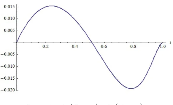
super-additive. However, as is shown in Figure 2.2, Pr(U2:3 ≤ t

)

−Pr(V2:3 ≤ t

)

is first

positive then negative on the interval [0,1], indicating that there is no stochastic order

between U2:3 and V2:3.

2.6 Identifying the NWUE order

As is seen in previous section, NWUE property of a random lifetime plays an important

Figure 2.2: Pr(U2:3 ≤t

)

−Pr(V2:3 ≤t

) .

build some methods to detect the strict NWUE order based upon two samples

Xn= (X1, . . . , Xn), Ym = (Y1, . . . , Ym)

from independent populations X and Y with continuous distributions, respectively.

2.6.1

Graphical method based on TTT plot

Define

φ−_F1(v) = 1 µF

∫ F−1(v)

0

¯

F(t) dt, v ∈(0,1),

the scaled total time on test (TTT) transform (see Barlow and Campo (1975)) of the distribution F of a random lifetimeX. Since F and φ−_F1 uniquely determine each other, TTT transform is convenient to be used to judge the aging properties of X. Bergman

(1979) showed that X is NWUE if and only if φ−_F1(v)≤v for all v ∈(0,1).

Example 2.6.1 (Pareto distribution) For the distribution in Example 2.3.1, it holds that

∫ G−1_(v)

0

¯

G(t) dt = β α−1

[

1−(1−v)1−1/v], v ∈(0,1).

0.2 0.4 0.6 0.8 1.0 0.2

0.4 0.6 0.8 1.0

shape parameter=100, 5, 2, 1.25

Figure 2.3: Scaled TTT plots of Pareto distributions with α = 100,5, 2, 1.25

φ−_G1(v) = 1−(1−v)1−1/v, v ∈(0,1).

It is evident that shape parameter α has a direct impact on the degree of NWUE

property whilst the scaled TTT transform is independent of the scale parameter β. As

can be seen in Figure 2.6.1, the smaller the shape parameter α, the more far below the

diagonal the scaled TTT transform, and hence the more NWUE the distribution is.

Let Fn(t) be the empirical distribution function, X1:n ≤ · · · ≤Xn:n be order statistics

and ¯X = 1_n∑n_i=1Xi be the sample mean ofX1,· · · , Xn. Then, for i= 1,· · · , n,

φ−_Fn1 (

i n

) = 1_¯

X

∫ Fn−1(i/n)

0

¯

Fn(t) dt= i

∑

j=1

Xj:n+ (n−i)Xi:n

n

∑

j=1

Xj:n

,

gives the sample version of the scaled TTT transform, which converges to the population

if its scaled TTT plot

( i n, φ

−1

Fn (

i n

))

, i= 1,· · · , n,

lies below the diagonal line.

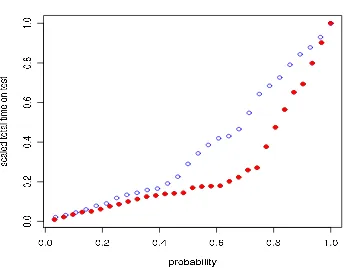
Example 2.6.2 (Proschan, 1963) Lifetimes (in hours) of the air-conditioning systems in two different planes are recorded in Table 2.6.2 below. TTT plots based upon these

plane’s type sample

8045 14,14,27,32,34,54,57,59,61,66,67,102,134,152,209,230 7909 10,14,20,23,24,25,26,29,44,44,49,56,59,60,61,62,

70,76,79,84,90,101,118,130,156,186,208,208,310

Table 2.1: Life times of air-conditioning systems of planes

lifetimes are listed in Figure 2.4. Apparently, they both are not below the diagonal line

Figure 2.4: TTT plots of air-conditioning systems in airplane: 8045 (◦), 7909 (•)

As a matter of fact, it is also quite convenient to identify the NWUE order by

com-paring the two TTT plots. It may be derived from (1.1) directly that

X ≥nwue Y if and only if φ−F1(v)≤φ−

1

G (v) for all v ∈(0,1).

Therefore, it is reasonable to identify the NWUE order through checking whether

( i n, φ

−1 Fn ( i n ))

, i= 1,· · · , n,

the TTT plot based onX1,· · · , Xn, lies below

( j m, φ

−1 Gm ( j m ))

, j = 1,· · · , m,

the TTT plot based onY1,· · · , Ym, here, forj = 1,· · · , m,

φ−_G1_m (

j m

) = 1_¯

Y

∫ G−m1(j/m)

0

¯

Gm(t) dt= j

∑

k=1

Yk:m+ (m−j)Yj:m

m

∑

k=1

Yk:m

,

Y1:m ≤ · · · ≤ Ym:m are order statistics and ¯Y is the sample mean corresponding to

Y1,· · · , Ym.

Example 2.6.3 (Skype and Yahoo) The users’ times (in seconds) of the network chat-ting systems are recorded in both Skype and Yahoo network chatchat-ting systems in Table

2.6.3.

As can be seen in Figure 2.5, the two TTT plots lie far below the diagonal

demon-strating the obvious NWUE property. Further, TTT plot of Skype system is below that

System sample

Yahoo 6,9,13,18,24,28,38,44,48,54,57,69,86,120,150,176, 198,206,234,306,400,447,502,604,708,800,1005,1560 Skype 2,5,8,11,12,15,19,22,26,30,34,36,39,40,41,52,55,57,

56,70,83,108,117,209,306,409,530,602,845,1203,1882

Table 2.2: Times user spend in chatting systems

2.6.2

A nonparametric test

In literature, some partial orders were introduced to measure various common aging

prop-erties, such as IFR, IFRA, NBU, DMRL and NBUE. However, they can not be accurately

detected without the parametric forms of survival functions. As a result, engineers resort

to statistical methods in practical applications. In the past decades, nonparametric

pro-cedures were proposed to test the IFR order, IFRA order, NBU order and DMRL order,

respectively. One may refer Aly (1993), Ahamed and Kochar (1990), Kusum et al (1986),

Hollander et al (1982) and Gerlach (1986), and Lai and Xie (2006) for more details. Here,

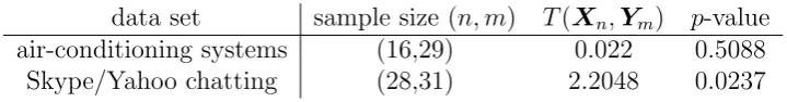
we propose a nonparametric test for the strict NWUE order.

According to Kochar and Wiens (1987), X ≥nwue Y and X ≤nwue Y (written as

X ∼ Y) if and only if ¯F(t) = ¯G(θt) for all t ≥ 0, where θ = µG/µF, µG = E[Y] and

µF = E[X]. That is, two random lives have same degree of NWUE-ness if and only if

their survival functions differ by at most a positive scale factor. In order to test the

following hypothesis

H: X ∼Y versus K: X ≥nwueY strictly,

it is necessary to build some testing statistic and derive its (asymptotic) null distribution.

Let

β(Y) = ∫ _∞

0

¯

G2(t) dt, β(X) = ∫ _∞

0

¯

F2(t) dt.

The following lemma helps to build a testing statistic for H versus K.

Proposition 2.6.4 If X ≥nwueY, then

∆(X, Y) = β(X) µF

− β(Y) µG

the strict inequality holds when X is strictly more NBUE than Y, that is, X ≥nwueY but

not X ∼Y.

Proof: X ≥nwueY impliesµF(F−1(s))≥θ−1µG(G−1(s)) for all 0≤s≤1. Then,

∫ 1

0

∫ _∞

F−1_(s)

¯

F(y) dyds = ∫ 1

0

µF(F−1(s)) ds

≥ 1

θ ∫ 1

0

µG(G−1(s)) ds

= 1 θ

∫ 1

0

∫ _∞

G−1_(s)

¯

G(y) dyds. (2.9)

By Fubini’s theorem, ∫ 1

0

∫ _∞

F−1_(s)

¯

F(y) dyds = ∫ _∞

0

∫ F(y)

0

¯

F(y) dsdy

= ∫ _∞

0

¯

F(y)F(y) dy

= E[X]− ∫ _∞

0

¯

F2(y) dy;

Likewise,

∫ 1

0

∫ _∞

G−1_(s)

¯

G(y) dyds =E[Y]− ∫ _∞

0

¯

G2(y) dy.

So, (2.9) implies

∫ _∞

0

¯

F2(y) dy− 1 θ

∫ _∞

0

¯

G2(y) dy≥E[X]− 1

θE[Y] = 0,

irrespective of the two meansµF and µG.

According to Proposition 2.6.4, ∆(X, Y) = 0 when X ∼ Y, and ∆(X, Y) > 0 when

X ≥nwue Y strictly. So, it serves as a reasonable measure for the deviation from the null

Let

β(Xn) =

( n 2

)−1∑n

i̸=j

min{Xi, Xj}, β(Ym) =

( m

2

)−1∑m

i̸=j

min{Yi, Yj}.

According to the theory of U-statistic (Hoeffding, 1948), if E[X4_{]<∞, then, as n→ ∞,}

√

n(β(Xn)−β(X)

)

2σX

L

−→ N(0,1),

where

σ_X2 =E[E[min{X1, X2}|X1]−β(X)]2.

By Slutsky’s theorem, it holds that, as n→ ∞, √

n [

β(Xn)

¯

X −

β(X) µF

]

2σX µF

L

−→ N(0,1). (2.10)

Likewise, as m→ ∞,

√ m

[

β(Ym)

¯

Y −

β(Y) µG

]

2σY µG

L

−→ N(0,1), (2.11)

where

¯ Y = 1

m

m

∑

i=1

Yi, σ2Y =E[E[min{Y1, Y2}|Y1]−β(Y)]2.

Combining (2.10) and (2.11), we reach the asymptotic distribution of

∆(Xn,Ym) =

β(Xm)

¯

X −

β(Yn)

¯ Y .

Proposition 2.6.5 Suppose E[X4_],E[Y4_{]<∞, and} m