A FRAMEWORK FOR DEBT-MATURITY
MANAGEMENT
Saki Bigio, Galo Nuño and Juan Passadore
Documentos de Trabajo
N.º 1919
A FrAmework For Debt-mAturity mAnAgement(*)
Saki Bigio (**)
UCLA
Galo Nuño (***)
BAnCo de espAñA
Juan Passadore (****)
eIeF
documentos de Trabajo. n.º 1919 2019
(*) The views expressed in this manuscript are those of the authors and do not necessarily represent the views of the Banco de españa or the eurosystem. The paper was influenced by conversations with Anmol Bhandari, Manuel Amador, Andy Atkeson, Adrien Auclert, Luigi Bocola, Alessandro dovis, Raquel Fernández, Hugo Hopenhayn, Francesco Lippi, Rody Manuelli, dejanir silva, dominik Thaler, Aleh Tsyvinski, pierre-olivier Weill, pierre Yared, dimitri Vayanos, Anna Zabai and Bill Zame. We thank davide debortoli, Thomas Winberry, and Wilco Bolt for discussing this paper. We also thank conference participants at sed 2017, nBeR summer Institute 2017, RIdGe 2017, Rome Junior Conference in Macroeconomics 2017, CseF-IGIeR symposium on economics and Insitutions, sIAM 2018 Meetings, the Restud Tour Reunion Conference, the CeBRA Annual Meeting 2018, and AdeMU sovereign debt Conference, and seminar participants at the Federal Reserve Board, Federal Reserve Bank of Chicago, Federal Reserve Bank of Cleveland, oxford, Banco de españa, penn state, essIM, sMU, snU, LUIss, UCLA, UT Austin, and eIeF, for helpful comments and suggestions.
The Working Paper Series seeks to disseminate original research in economics and fi nance. All papers have been anonymously refereed. By publishing these papers, the Banco de España aims to contribute to economic analysis and, in particular, to knowledge of the Spanish economy and its international environment.
The opinions and analyses in the Working Paper Series are the responsibility of the authors and, therefore, do not necessarily coincide with those of the Banco de España or the Eurosystem.
The Banco de España disseminates its main reports and most of its publications via the Internet at the following website: http://www.bde.es.
Reproduction for educational and non-commercial purposes is permitted provided that the source is acknowledged.
© BANCO DE ESPAÑA, Madrid, 2019
Abstract
We characterize the optimal debt-maturity management problem of a government in a small open economy. The government issues a continuum of fi nite-maturity bonds in the presence of liquidity frictions. We fi nd that the solution can be decentralized: the optimal issuance of a bond of a given maturity is proportional to the difference between its market price and its domestic valuation, the latter defi ned as the price computed using the government’s discount factor. We show how the steady-state debt distribution decreases with maturity. These results hold when extending the model to incorporate aggregate risk or strategic default.
Keywords:debt maturity, debt management, liquidity costs.
Resumen
En este trabajo se determina el problema de la gestión óptima de la deuda pública en una pequeña economía abierta. El Gobierno emite un continuo de bonos de vencimiento fi nito sujeto a restricciones de liquidez. Hallamos que la solución puede ser descentralizada: la emisión óptima de un bono de un vencimiento dado es proporcional a la diferencia entre su precio de mercado y su valoración doméstica, esta última defi nida como el precio obtenido empleando la tasa de descuento del Gobierno. Mostramos que la distribución de deuda en el estado estacionario disminuye con el vencimiento. Estos resultados se mantienen si extendemos el modelo para incorporar riesgo agregado o impago estratégico.
Palabras clave:vencimiento de la deuda, gestión de la deuda, costes de liquidez.
CONTENTS
Abstract 5
Resumen 6
1 Introduction 8
2 Maturity management with liquidity costs 14
2.1 Model setup 14
2.2 Solution: the debt issuance rule 17 2.3 Asymptotic behavior 20
2.4 The cases without liquidity costs and vanishing liquidity costs 22 2.5 Calibration 23
2.6 Maturity management with unexpected shocks 25
3 Risk 30
3.1 The model with risk 31
3.2 Solution: risk-adjusted valuations 32 3.3 The risky steady state 34
4 Default 36
4.1 The option to default 37 4.2 Default-adjusted valuations 38
4.3 The impact of default on maturity choice 41
5 Extensions 44
5.1 Alternative specifi cations for the liquidity costs 44 5.2 Finite issuances 44
5.3 Consols 45
6 Conclusions 46
References 47
Appendix: A Framework for Debt-Maturity Management 53
A Equivalence between PDE and integral formulations 54 B Micro model of liquidity costs 55
C Proofs 59
D Calibration notes 79
E Some stylized facts bond issuances in Spain 81 F Computational method 89
This rule states that the optimal issuance of a bond of a given maturity is the ratio of a relative value gap to the liquidity coefficient. The relative value gap of a bond of a given maturity is the difference between the bond price in the secondary market and the domestic valuation, rel-ative to the secondary market price. The domestic valuation is the counterfactual bond price computed using the government’s discount factor, which differs from the international
short-1This limitation is easily understood with a simple example. If we want to construct a yearly model where the government issues a single 30-year, zero-coupon bond, we need at least 30 state variables: a 30-year bond becomes a 29-year bond the following year, and a 28-year bond the year after, and so on. By contrast, a bond that matures by 5 percent every year is still a bond that matures by 5 percent the year after its issuance.
1
Introduction
How should a government manage its debt maturity structure? This paper presents a new framework to think about maturity management. The framework makes two innovations. First, it puts forth the importance of liquidity frictions, namely the notion that the larger an issuance at a given maturity the lower the price. Liquidity costs have been well documented by the empirical literature, but have received much less attention by normative theory. The second innovation is technical. The curse of dimensionality quickly restricts the number and class of bonds that can be considered in debt-management problems. Quantitative studies typ-ically model bonds that mature exponentially and work with two maturities only.1 In practice, however, governments issue finite-life bonds in many maturities. The framework here allows us to work with any number of bonds of arbitrary coupon structure.
The goal of the framework is to analyze an optimal debt-maturity design in the presence of liquidity frictions. To this end, we lay out a continuous-time, small open economy. A relatively impatient government chooses to issue or (re-)purchase finite-life bonds within a continuum of maturities. Its financial counterparts are risk-neutral international investors. The government’s objective is to smooth consumption. It faces income and interest rate risk and can default when those risks materialize. Liquidity costs emerge because bonds are auctioned to primary dealers that need time to liquidate their bond holdings after an auction. The bond market is segmented across maturities and vintages, in the spirit of Vayanos and Vila (2009). Under these assump-tions, the larger the auction, the lower the price. The induced price impact is summarized by a single coefficient that increases with the holding costs of intermediaries, but decreases with the size of order flows.
We characterize the solution to the government’s problem and show that the optimal is-suance problem can be decentralized. Namely, the problem can be studied as if the govern-ment delegates issuances to a continuum of subordinate traders, each in charge of managing a single maturity. Each trader then applies a simple rule to determine how much to issue of his maturity:
issuance at maturity
GDP =
2The government’s discount factor is computed as the solution of a fixed-point problem in the path of con-sumption. An imputed consumption path maps to a government discount factor. This discount factor generates a path for debt through the issuance rule. Ultimately, the path for debt produces a new consumption path. In the optimal solution, both consumption paths must coincide.
term rate.2 A positive value gap indicates that the trader in the decentralization scheme would otherwise issue as much debt as possible. That desire is contained by the liquidity costs, cap-tured by the liquidity coefficient, which reduce prices in the primary market. We calibrate the liquidity coefficient using data on turnover rates and intermediation spreads.
The paper is built in layers. In the first layer, we study the problem under perfect foresight, in the second layer we add risk, and in the final layer, we add the option to default. Under perfect foresight, the asymptotic dynamics of the model can be obtained analytically. Provided that liquidity costs are above a certain threshold, the model features a steady state. In the steady state, the government issues at all maturities, but issues greater quantities of long-term bonds. It is optimal to issue at all maturities because liquidity costs are convex, namely the price impact increases with the issuance. The steady-state maturity structure is determined by the desire to spread out issuances to minimize the liquidity costs. Nonetheless, this desire does not produce a uniform issuance distribution. This is because long-term bonds have to be rolled over less frequently than short-maturity ones and, hence, the use of the former is preferable in order to minimize rollover costs. Although issuance flows increase with maturity, the outstanding stock of debt decreases with maturity. This decreasing maturity profile for the debtstockis an artifact of bonds having a finite life: as long-term bonds mature, they become short-term bonds. Thus, at steady state, the stock of debt at a given maturity is the accumulation of the issuance flows at higher maturities. We calibrate the model for the case of Spain and obtain a debt profile that resembles that in the data.
We use the framework to characterize the maturity distribution as liquidity frictions vanish. Although there is no steady state distribution below a threshold value of the liquidity coeffi-cient, there always exists a well-defined asymptotic debt distribution. This limit-determinacy result contrasts with the case without liquidity costs, in which the maturity profile is indeter-minate.
We also study the transitional dynamics after an unexpected shock. Two forces interact with the liquidity costs to shape the dynamics: consumption smoothing and bond-price reaction.
Consumption smoothing is activated when the path of consumption growth changes the do-mestic discount factor. As a result, dodo-mestic valuations are modified. Consumption smoothing lengthens the maturity during downturns: after a shock produces a temporary drop in con-sumption, the domestic discount rate remains temporarily high while the economy recovers. This reduces domestic valuations, particularly for longer maturities. The optimal rule thus pre-scribes the issuance of more debt, especially at longer maturities. The economic intuition is that the government issues more debt during recessions to smooth consumption, especially at longer maturities to avoid the liquidity costs associated with the rollover of debt.
do-3The concept of RSS is equivalent to the one that appears in Coeurdacier et al. (2011). The analysis of the RSS is
theonlytractable solution that does not rely on approximations. Transitional dynamics prior to the shock are not analytically tractable.
mestic discount factor coincides with the market interest rate, and the government is indifferent between issuing debt at any two maturities. With liquidity costs, however, the government is not indifferent, as rebalancing between different maturities is costly. If a shock temporarily increases short-term rates, thereby reducing market prices—especially for long maturities, the optimal rule dictates, ceteris paribus, a decline in debt issuances and the tilting of the matu-rity distribution toward shorter maturities. The government thus reduces the issuance of those bonds most affected by the temporary fall in prices. The initial shock produces a decline and posterior recovery in consumption, which activates consumption smoothing —a force that par-tially mitigates bond-price reaction.
The next layer incorporates risk. Because the state variable is the entire maturity distribu-tion, the characterization of an equilibrium with recurrent shocks faces the same computational challenge as incomplete market models with heterogeneous agents and aggregate shocks (as in Krusell and Smith, 1998, and subsequent literature). To provide an analysis of the government’s problem with risk that does not rely on numerical approximations, we study an economy where shocks are anticipated, but occur only once. This approach is useful because we can characterize the risky steady state (RSS), defined as the steady state reached when the government expects a shock, but the shock has not yet materialized.3 Through the analysis of the RSS, we can study how the anticipation of risk shapes the maturity distribution. We show that the government follows the same issuance rule as in the deterministic case. The anticipation of risk introduces an extra term into the domestic valuations: expected valuations after the shock arrival are ad-justed by the ratio of post- to pre-shockmarginal utilities, reflecting an effective "exchange rate" between consumption goods at different states.
Risk introduces a new force that influences the maturity distribution, insurance. Insurance shapes the maturity profile in two ways. First, the government tries to build a hedge. In the ab-sence of liquidity costs, the government mayhedgethe changes in consumption due to interest rate shocks by building a portfolio that offsets the impact of the shock. Liquidity costs make a perfect hedge—a hedge that guarantees equal consumption in all states— too costly. Second, the government tries toself insure. Self-insurance shows up in the ratio of marginal utilities be-cause a future drop in consumption increases that ratio and, thus, raises valuations. By raising valuations, self-insurance produces a lower stock of debt in the RSS than in the deterministic steady state (DSS). Self insurance-lengthens the average maturity because long-term bonds are less likely to have expired by the time a shock arrives, thus reducing the expected liquidity costs of debt rollover under a negative shock. Although both hedging and self-insurance are
present, our calibration shows that self-insurance is a stronger force.
4There is substantial evidence of liquidity costs in different asset classes, as surveyed by Vayanos and Wang
(2013b) or Duffie (2010). In the specific case of fixed-income securities, studies that provide evidence suggestive of the presence of liquidity costs are Cammack (1991), Duffee (1996), Spindt and Stolz (1992), Fleming (2002), Green (2004), Pasquariello and Vega (2009), Krishnamurthy and Vissing-Jorgensen (2012), Lou et al. (2013), and Song and Zhu (2018) for US Treasury markets, by Duffie et al. (2003), Naik and Yadav (2003b), Pelizzon et al. (2016) and Breedon (2018) for sovereign bond markets, Edwards et al. (2007) and Feldhutter (2011) for US corporate bond markets, and Green et al. (2007) for US municipal bond markets. Our calibration is based on inventory-depletion evidence in the US Treasury market documented by Fleming and Rosenberg (2008).
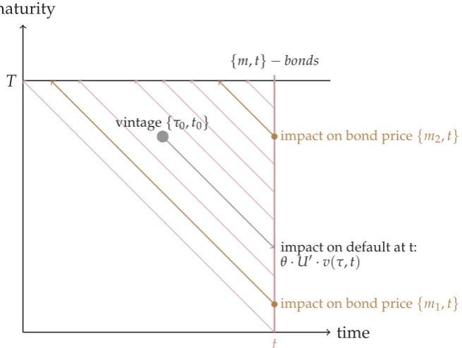
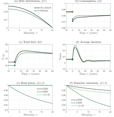
a higher value than repayment. Once again, the optimal issuance rule determines the matu-rity profile, but default changes bond prices and valuations. Both bond prices and valuations are corrected by a default risk premium. However, domestic valuations are also adjusted by an additional term, which does not appear in the market price of bonds. We dub this term the revenue-echo effect. The revenue-echo effect appears because, in the decentralization of the problem, traders anticipate that a marginal rise in their issuances increases default probabili-ties during the life of the bond. The increase in default risk in future periods echoes back in time through the prices of all bonds that are outstanding during the life of the bond. This fall in bond prices reduces revenue collections from other issuances. All in all, the revenue-echo effect incorporates the spillover of default risk from one bond to the rest of the portfolio. We analyze how the option to default shapes the maturity distribution at the RSS and find that, for our calibration, the revenue-echo effect dominates all the other forces in shaping the maturity distribution.
A similar revenue-echo effect would appear in a version of the model where liquidity costs depend on the outstanding stock of debt, and not only on issuances, as we study here. The so-lution with default showcases that the techniques are portable to more general environments. Indeed, section 5 explores several variations and applications of the model, namely (i) alterna-tive specifications of liquidity costs, (ii) the case of a government that can only issue debt at a finite number of maturities, and (iii) the issuance of consols instead of finite-life bonds.
Related literature. Maturity management appears in various areas of finance: international, public, and corporate. The framework here captures forces that have been previously identified and uncovers new ones. An advantage of the framework is that it allows for a large number of securities with a realistic coupon structure.
5See for example Arellano (2008) and Aguiar and Gopinath (2006), and Aguiar and Amador (2013) and Tomz
and Wright (2013) for recent reviews.
6Hatchondo and Martinez (2009), Chatterjee and Eyigungor (2012), and Chatterjee and Eyigungor (2015) study
quantitatively the positive and normative properties of a model in which the government borrows by issuing long term bonds, a setup that is prone to debt dilution.
bonds to investors. Our framework can, however, also be used to study maturity management problems without liquidity costs.
International finance stresses several forces that, in our framework, interact with the liq-uidity costs and shape the maturity structure. One force is insurance. A small open economy effectively has access to complete markets when income shocks are correlated with shocks to the yield curve in a way that allows complete asset spanning, as illustrated by Duffie and Huang (1985). With complete spanning, the optimal maturity design is governed by the formation of a bond-portfolio hedge that insulates the country against income and interest rate risk. But if income shocks are uncorrelated with interest rate shocks, the government cannot exploit the maturity of its portfolio to hedge. In that case, the debt dynamics are governed by self-insurance only, as in Chamberlain and Wilson (2000) or Wang et al. (2016). In between these extremes, there are a range of cases with incomplete asset spanning with a role for both hedging and self-insurance. In our framework, liquidity costs inhibit perfect hedges, so self-insurance and partial hedging interplay to shape the debt-maturity profile, independently of the asset structure.
The second force stressed by international finance isincentives. When the government has the option to default, it should take into consideration how current issuance affects the incen-tives to default in the future and how future default affects current prices. This feature was first introduced in a sovereign debt model by Eaton and Gersovitz (1981), and a large literature has followed.5 The effect of incentives in our framework is captured by the revenue-echo effect. The literature has further identified two important channels, which we abstract from, through which incentives shape the optimal maturity design. The first channel is debt dilution. Bulow and Rogoff (1988) identified that, without commitment to a debt program, long-term debt is prone to debt dilution. Debt dilution occurs when the price of outstanding bonds fall as a re-sult of a new issuance. The expectation of debt dilution raises the cost of long-term debt. Debt dilution is a force tilting issuances toward short maturities.6 The second channel, rollover risk, operates in the opposite direction. Cole and Kehoe (2000) identified that a solvent government faces rollover risk if it cannot refinance a large amount of principal and, as a result, is forced
to default. Rollover risk is a force toward spreading debt services through many maturities to avoid a large principal payment at any given point.
7Dovis (Forthcoming) studies the optimal risk sharing agreement when the government lacks commitment
and income is not verifiable, and shows that empirical features documented and rationalized by the quantitative literature on sovereign borrowing naturally emerge as constrained-efficient outcomes in this setup.
8Two alternative frameworks allow for richer debt structures, Sánchez et al. (2018) and Bocola and Dovis (2018).
In Sánchez et al. (2018) the government chooses each period total debt and the number of periods to repay this debt in equal installments. In our formulation, this choice corresponds to flat debt maturity profiles that differ in their average duration. In Bocola and Dovis (2018), instead, the government chooses each period total debt and a rate of decay for future promised payments. In both papers, total debt plus an additional state variable (number of periods or rate of decay) are sufficient to describe debt maturity profiles. By constrast, in our paper, we allow in principle for any debt maturity profile.
9Barro (2003) considers a tax-smoothing objective to assess the optimal maturity structure of public debt. property that, under debt dilution, once the country has issued long-term debt, it should let long-term bonds mature rather than refinance them with short-term debt. Further recent con-tributions that combine insurance, incentives, and rollover risk include, for example, Aguiar et al. (2017) and Bocola and Dovis (2018).7
Our paper abstracts away from debt dilution and rollover risk, but contributes to the afore-mentioned literature along two dimensions. First, as we explained earlier, most of the models employed by this literature restrict the number and types of bonds issued. Our framework presents a methodology in which debt problems can be analyzed without these restrictions. In light of the previous discussion, restrictions on the number of bonds and coupon structure represent a limitation of the sovereign debt literature. For example, if debt dilution is present, hedging may be very expensive if long-term debt is restricted to only bonds of very long matu-rities. Similarly, rollover risk can be mitigated if the country can spread out its issuances, and is not restricted to a few bonds. By circumventing these ad-hoc restrictions, we believe our frame-work is a step toward understanding debt management with realistic debt structures, where the government is allowed to design its debt profile to mitigate these incentive problems.8 Second, this paper is the first to solve the debt management problem under commitment to a debt pro-gram. This case is a natural and useful benchmark. It is natural if we think that an independent agency controls the debt maturity profile or if an international organization has a discipline device on a sovereign. It is also a useful benchmark to obtain an upper bound on the welfare gains if we want to establish the benefits from a fiscal rule.
Maturity choice is also a classical theme in public finance models. Models of taxation with commitment, as in Lucas and Stokey (1983), Angeletos (2002) or Buera and Nicolini (2004), show how a menu of bonds that differ in maturity implements a complete market allocation.9 Buera and Nicolini (2004) also show that this implementation results in unrealistic debt flows and positions.10 In our paper, because of the liquidity costs, portfolios have to be rebalanced very smoothly and this induces less extreme positions. Recently, Debortoli et al. (2017) and Debortoli et al. (2018) study maturity choice in similar environments but when the govern-ment lacks commitgovern-ment. These papers show that the governgovern-ment chooses a maturity structure that is approximately flat. Our framework generates allocations that are tilted toward shorter
10 Faraglia et al. (2010) show that introducing habits and capital leads leads to bond positions that are even
g
11Maturity choice is also a recurrent theme in corporate finance. Leland and Toft (1996) introduce a stationary
debt structure, which has been widely adopted in the literature that studies the optimal capital structure. Recent contributions that study optimal maturity choice are, for example, Chen et al. (2012), He and Milbradt (2016) and Manuelli and Sánchez (2018). Our framework can be adapted to answer questions in public or corporate finance.
12Recent examples are Bhandari et al. (2017a) and Bhandari et al. (2017b). The first paper shows how the
gov-ernment chooses debt, asymptotically, to minimize the variability of fiscal shocks, defined as the sum of the return on debt and spending shocks. The second paper, building on the previous results, shows that when the model is calibrated using US returns on debt and primary deficits, the optimal maturity of debt does not involve any short positions.
maturities which, in our calibrated exercise, are quantitatively similar to those of the Spanish government.11
Our paper is also close to the literature that studies tax smoothing under incomplete markets following Aiyagari et al. (2002).12 Faraglia et al. (Forthcoming) introduce a new method to solve an extension of Aiyagari et al. (2002) that allows for several finite-life bonds of different maturities. In contrast, our paper develops an analytical method to characterize the solution. Our method allows for a clear decomposition of the different economic forces that shape the debt distribution in response to shocks. A common aspect with Faraglia et al. (Forthcoming) is the importance of liquidity costs to obtain a realistic debt profile.
On the technical front, the framework employs infinite-dimensional optimization techniques similar to those applied in heterogeneous agent models. Lucas and Moll (2014) study a problem with heterogeneous agents that allocate time between production and technology generation. Nuño and Moll (2018) study a constrained-efficient allocation in a model with heterogeneous agents and incomplete markets. Nuño and Thomas (2018) study optimal monetary policy in a heterogeneous-agent model with incomplete markets and nominal debt. The contribution rel-ative to those studies is that this paper introduces the risky steady-state approach to study the impact of aggregate risk. This feature is novel, and allows for an exact characterization that can be used to analyze models with aggregate risk.
2.1
Model setup
Time is continuous. The model features two exogenous state variables, {y(t),r∗(t)}t≥0, rep-resenting an endowment and a short-term interest rate process, respectively. The vector of exogenous states is X(t) ≡ [y(t),r∗(t)]. For any variable, whether endogenous or exogenous, we employ the notation x∞ ≡ limt→∞x(t) to refer to its asymptotic value and xss to refer to its steady state value, if it exists. In the case of the exogenous state variables, we use both sub-scripts indistinctly. All the partial differential equations (PDE) that we present here have exact solutions which are presented in Table A of Appendix A.
Households. We consider a small open economy. There is a single, freely-traded consump-tion good. The economy is populated by a representative household with preferences over expenditure paths,{c(t)}t≥0, given by
V0 = ˆ ∞
0
e−ρtU(c(t))dt,
where ρ ∈ (0, 1), rss∗ < ρ, is the discount factor andU(·) is an increasing and concave utility function.
Government. The economy features a benevolent government that issues bonds to foreign investors on behalf of households. Bonds differ by their time to maturity. The time to maturity of a given bond is denoted by τ. Issuances are chosen from a continuum of maturities, τ ∈ [0,T], where T is an exogenous maximum maturity. The maturity of a given bond falls with time, ∂τ∂t = −1, and the bond is retired once it matures,τ = 0. At maturity, the bond pays its principal, normalized to one unit of good. Prior to maturity, the bond pays an instantaneous
constant coupon δ. As we discuss in section 5, our framework can also accommodate bonds
with different coupon rates. However, for simplicity, we focus on the case in which all bonds have the same coupon rate.
The outstanding stock of bonds with a time-to-maturityτat datetis denoted by f (τ,t). We call{f (τ,t)}τ∈[0,T]the debt profile at timet. The law of motion of f (τ,t)follows a Kolmogorov forward equation (KFE):
∂f
∂t =ι(τ,t) +
∂f
∂τ, (2.1)
with boundary condition f(T,t) = 0. The intuition behind the equation is that, givenτ andt, the change in the quantity of bonds of maturityτ, ∂f/∂t, equals the issuances at that maturity,
ι(τ,t), plus the net flow of bonds,∂f/∂τ. The latter term captures the aging of the outstanding bonds, i.e., the automatic flow from longer to shorter maturities. Issuances, ι(τ,t), are cho-sen from a space of functions I : [0,T]×(0,∞) → R that meets some technical conditions.13 When negative, issuances are interpreted as bond purchases or repurchases. The initial stock ofτ−maturity debt is given, f(τ, 0) = f0(τ). The government’s budget constraint is:
c(t) = y(t)− f (0,t) +
ˆ T
0 [
q(τ,t,ι)ι(τ,t)−δf (τ,t)]dτ, (2.2)
where y(t) is the (exogenous) output endowment, with steady state value yss. Furthermore, −f (0,t) is the principal repayment, δ´0T f dτ are total coupon payments from all outstanding bonds, and´0Tqιdτare the funds received from debt issuances at all maturities. Finally,q(τ,t,ι) is the issuance price of a bond of maturity τ at date t in the primary market. As we discuss below, the price depends on the total volume of issuances of that maturityτ.
14See Foucault et al. (2013) for a textbook treatment of liquidity and market micro-structure and Stoll (2003),
Madhavan (2000) and Vayanos and Wang (2013a) for reviews. The three main economic forces explored by this literature are: (i) inventory management of financial intermediaries, (ii) adverse selection and, (iii) order processing costs. Seminal inventory problem papers are Ho and Stoll (1983), Huang and Stoll (1997), Grossman and Miller (1988), and Weill (2007). In the case of adverse selection, see Glosten and Milgrom (1985), Kyle (1985) or Easley and O’hara (1987). A general reference of the implications of order processing costs is Foucault et al. (2013). A large empirical literature has documented the presence of price impact. For example, see Madhavan and Smidt (1991), Madhavan and Sofianos (1998), Hendershott and Seasholes (2007) or Naik and Yadav (2003a,b).
International investors. The government trades bonds with competitive risk-neutral inter-national investors. The issuance price,q, has two components, a frictionless market price and a liquidity cost:
q(τ,t,ι) = ψ (τ,t)
market price
− λ (τ,t,ι) liquidity costs
. (2.3)
The first component,ψ(τ,t), is the arbitrage-free market price of the domestic bond. This price depends on the path of the international risk-free interest rate,r∗(t). Given this risk-free rate, the market priceψ(τ,t)has a PDE representation:
r∗(t)ψ(τ,t) =δ+ ∂ψ
∂t −
∂ψ
∂τ, (2.4)
with a boundary conditionψ(0,t) = 1. Unless indicated otherwise, we assume thatδ =r∗ss. Liquidity costs. The second component in the issuance price,λ(τ,t,ι), represents aliquidity costassociated with the issuance (or purchase) ofιbonds of maturityτat datet. In Appendix B, we present a wholesale-retail model of the bond market, whose solution yields the formulation of the liquidity cost that we employ throughout the paper. This is similar in spirit to models that feature over-the-counter (OTC) frictions, like Duffie et al. (2005). The main virtue of this friction is that it produces a price impact of issuances, which has been extensively documented in asset markets.14
In particular, we assume that to issue bonds of maturityτat datet, the government decides
to auctionι(τ,t)bonds. The participants in that auction are a continuum of investment bankers. Bankers participate in the auction and buy the total bond issuance. This is the wholesale market. Then, bankers offload bonds to international investors in a retail (secondary) market. As in Duffie et al. (2005), bankers have higher costs of capital than investors. In particular, bankers’ cost of capital isr∗(t) +η, whereη >0 is an exogenous spread. In the retail market, bankers are continuously contacted by investors. The contact flow is μyss per instant. Each contact results in an infinitesimal bond purchase by investors from a banker’s bond inventory. Thus, in an interval Δt, the stock of bonds sold by the banker isμyssΔt. We assume that bankers extract all the surplus from the international investors.
Thus, the approximate liquidity cost function isλ(τ,t,ι) ≈ 21λψ¯ (τ,t)ι. The term ¯λis a liquidity cost coefficient which increases with the spread and decreases with the contact flow.
More General Liquidity Costs. An implicit assumption behind this formulation is that there are no congestion externalities: the contact flow is independent of the outstanding debt at a given maturity. We may consider two departures to this case. First, we could allow for a price impact that spills across maturities and, in that case, equation (2.5) would depend on the entire issuance function, ι(·,t), and not only the issuance at a given maturity. This departure would still feature liquidity costs that depend on issuances. A second departure would be to allow for liquidity costs that depend on the stock of outstanding debt. In principle our methodology can also deal with that situation. In fact, the solution would share a similarity with the case of default analyzed in section 4. We discuss this connection again in section 5.
We now return to the government’s problem and make no further reference to the source of the liquidity costs.
L[ι, f] =
ˆ ∞
0
e−ρtU
y(t)− f(0,t) +
ˆ T
0 [
q(t,τ,ι)ι(τ,t)−δf(τ,t)]dτ
dt
+ ˆ ∞
0 ˆ T
0
e−ρtj(τ,t)
−∂∂f
t +ι(τ,t) +
∂f
∂τ dτdt,
15An alternative approach to solving for the optimal solutions, proposed by Golosov et al. (2014), Sachs et
al. (2016), and Tsyvinski and Werquin (2017), is to analyze the welfare gains of perturbations from (potentially suboptimal) policies observed in practice.
market price ψ(τ,t). These properties are common to OTC models, e.g., Duffie et al. (2005). In Appendix B, we present an exact solution to the auction price as a function of the market price and the issuance size. Here we present an approximation, a first-order Taylor expansion aroundι =0, which yields a convenient linear expression for the auction price:
q(ι,τ,t) ≈ψ(τ,t)−1
2
η μyss
¯
λ
ψ(τ,t)ι(τ,t). (2.5)
V[f (·, 0)] = max
{ι(τ,t),f(τ,t),c(t)}t≥0,τ∈[0,T] ˆ ∞
0
e−ρtU(c(t))dt, (2.6)
Government problem. The government maximizes the utility of the households given by
subject to the law of motion of debt (2.1), the budget constraint (2.2), the initial condition f0and debt prices (2.3). The object V is thevalue functional, which maps the initial debt profile given by f0, into a real number. It is a functional because the state variable is infinite-dimensional.15
2.2
Solution: the debt issuance rule
where we substitute consumption and bond prices from the objective function using the budget constraint (2.2) and the bond price schedule (2.3). The second line is the law of motion of the debt distribution, to which we attach the Lagrange multiplierj(τ,t). The necessary conditions are obtained by a classic variational argument. The idea is that, at the optimum, the optimal issuance and debt paths cannot be improved. A first condition is that no infinitesimal variation around the controlιcan produce an increase in the Lagrangian. This implies that:
U(c(t))
q(t,τ,ι) + ∂q
∂ιι(τ,t) =−j(τ,t). (2.7)
This necessary condition is intuitive: the issuance of a(τ,t)-bond produces a marginal cost and a marginal benefit, and both margins must be equal at an optimum. The marginal benefit is the marginal utility of the marginal increase in consumption, which equals the average price of that bond,q, plus the price impact of an additional issuance, ∂∂ιqι. The marginal cost of the issuance is summarized in the Lagrange multiplier,−j, which captures the forward-looking information on the bond repayment, as explained next.
A second condition is that no infinitesimal variation over the state f can yield an improve-ment in value. The solution cannot be improved as long as the Lagrange multipliers j satisfy the following PDE:
ρj(τ,t) = −U(c(t))δ+∂j
∂t −
∂j
∂τ, τ ∈ (0,T], (2.8)
with a boundary condition: j(0,t) =−U(c(t))and a transversality condition limt→∞e−ρtj(τ,t) = 0.
Each Lagrange multiplier is forward-looking because it captures future repayment costs in the form of a continuous-time present-value formula. The first term,−U(c(t))δ, is a disutility flow associated with the marginal cost of coupon payments. The second and third terms,∂j/∂t
and∂j/∂τ, capture the change in flow utility as time and the maturity of the bond progress. For interpretation purposes, it is convenient to translate the multiplierjfrom utils into consumption units. This change of units is useful to transform each multiplier into a financial cost. Define a transformed multiplier asv(τ,t) ≡ −j(τ,t)/U(c(t)). We refer to vas thedomestic valuation
of a (τ,t)-bond. Aided with this definition, we re-express the first-order conditions (2.7) and (2.8) as
∂q
∂ιι(τ,t) +q(t,τ,ι) = v(τ,t), (2.9)
and the PDE,
r(t)v(τ,t) = δ+∂v
∂t −
∂v
∂τ, ifτ ∈(0,T], (2.10)
with terminal conditionv(0,t) =1. The rater(t)is defined as
r(t) ≡ρ−U
(c(t))c(t)
U(c(t))
.
c(t)
Different from r∗(t), the rate r(t) is the infinitesimaldomestic discount factor. Under Constant Relative Risk Aversion (CRRA) utility,U(c) = c1−1−σ−σ1, the domestic discount factor satisfies the classical formular(t) =ρ+σc˙(t)/c(t). There is a remarkable connection between the domestic valuation (2.10) and the market-price equations (2.4): both are net present values of the cash flows associated with each bond, the only difference between them is the interest rate used to discount the flows. The market price of the bond is computed discounting at r∗, whereas the domestic valuation uses r. The optimal issuances given by (2.9) depend on the spread between the two valuations. The next proposition summarizes the discussion and provides a full characterization of the solution:
Proposition 1. (Necessary conditions) If a solution{c(t),ι(τ,t), f (τ,t)}t≥0 to (2.6) exists then do-mestic valuations satisfy equation (2.10), optimal issuances ι(τ,t) are given by the issuance rule (2.9) and the evolution of the debt distribution can be recovered from the law of motion for debt, (2.1), given the initial condition f0. Finally, c(t) and r(t) must be consistent with the budget constraint (2.2) and
the formula for the internal discount, (2.11).
Proof. See Appendix C.1.
The rule states that the optimal issuance of a(τ,t)-bond should equal the product of the value gap and the inverse liquidity coefficient. This value gap is the difference between the market price,ψ, and the domestic valuation of a bond, v, relative to the market price. When the value gap is positive, a trader wants to issue debt because the market price exceeds the valuation of that debt. A force contains the desire to issue, the liquidity cost, which captures the reduction in price as the issuance becomes larger. This force appears as the coefficient 1/ ¯λ. The lower ¯λ, the greater the issuance.
The government’s problem has adualcost-minimization representation. The dual problem minimizes the net present value of financial expenses, given the discountr(t)constructed out of a desired consumption pathc(t). Formally, the dual problem is:
min
{ι(τ,t)}t≥0,τ∈[0,T] ˆ ∞
0
e−´0tr(s)ds
f (0,t) +
ˆ T
0 δ
f (τ,t)dτ−
ˆ T
0
q(τ,t,ι)ι(τ,t)dτ
dt (2.13)
There are two noteworthy features of the solution. The first feature is adecentralizationresult: We can interpret the solution as if the government designates a continuum of traders, one for eachτ, to give an domestic price to its debt, given the domestic discount factor r. Each trader then issues debt according to the rule in (2.9). The discount factor, of course, must be internally consistent with the consumption path produced by issuances.
The second feature is that issuances are given by a simple debt issuance rule. Considering the liquidity cost function (2.5), the optimal-issuance condition (2.9) can be written as:
ι(τ,t) = ψ(τ,t)−v(τ,t)
ψ(τ,t)
.
value gap
1 ¯
λ
1/liquidity coefficient
2.3
Asymptotic behavior
The long-run behavior of the solution can be characterized analytically, as shown in Appendix C.3. In some instances, the solution reaches a steady state and in others the solution converges asymptotically to zero consumption. Whether there is a well-defined steady state with positive consumption depends on the value of ¯λ. In particular, we obtain an expression for thethreshold
value ¯λo. A steady state exists if and only if ¯λ > λ¯o. If ¯λ ≤ λ¯o, there is no steady state;
∂ιss
∂τ =
ρ−r∗ss
¯
λ e−ρτ >0.
wherer(t)is given by (2.11), the minimization is subject to the law of motion of debt (2.1) and the initial condition f0, and debt prices satisfy (2.3). The expression in parentheses is the net flow of financial receipts. This dual problem is consistent with a debt-management office man-date to minimize the financial expenses of a given expenditure path. The proof is in Appendix C.2.
consumption decreases asymptotically at the exponential rate r∗ss−ρ and r(t) converges to a limit value r∞λ¯. The asymptotic discount factor r∞λ¯ is increasing and continuous in ¯λ
with boundsr∞λ¯o
=ρandr∞(0) =r∗ss.
In the case where ¯λ > λ¯o, the solution renders an analytic expression for the steady state,
with market prices and valuations:
ψss(τ) = δ1−e
−rss∗τ r∗ss +e
−r∗ssτandv
ss(τ) =δ1−e
−ρτ
ρ +e−ρτ. (2.14)
Assuming that δ = r∗ss, all bonds are issued at par, ψss(τ) = 1, andvss(τ) = r∗ss1−e
−ρτ
ρ +e−ρτ.
Issuances at steady state,ιss(τ), follow from (2.12), and the outstanding debt satisfies
fss(τ) =
ˆ T
τ ιss(s)ds, (2.15)
so their expressions are given by:
ιss(τ) = ρ−r
∗
ss
ρλ¯
1−e−ρτ, and fss(τ) = ρ−r
∗
ss
ρλ¯
ˆ T
τ
1−e−ρsds. (2.16)
There is no issuance at the shortest maturity,ιss(0) = 0, because domestic valuations coincide
with market prices. Differences in valuations are higher for longer maturities, as the govern-ment discounts future cash flows at a rate ρ greater than r∗ss, whereas the market price of all bonds is constant and equal to 1. This means that, at the margin, the government is willing to receive a lower price on a long-maturity bond, because it requires less frequent retrading.
By contrast to the maturity distribution of issuances, that of debt is decreasing in maturity. The reason is simple: because debt is the integral of issuances (see equation2.15), it should be decreasing in maturity as long as issuances are positive, which is guaranteed by the fact that
16These two results regarding issuance are a direct consequence of the fact, explained in Appendix C.3, that the
limit discount factor isr∗ss ≤ r∞λ¯ ≤ ρand hence limT→∞ι∞(τ;T) = r∞(
¯
λ(T))−r∗ss
r∞(λ¯(T))λ¯(T)
1−e−r∞(λ¯(T))τ = 0 and
∂ι∞
∂τ = r∞(
¯
λ(T))−r∗ss
¯
λ(T) e−ρτ>0 with limT→∞
∂ι∞
∂τ =0. In the limit, the domestic discount converges to the risk-free rate,
limT→∞r∞λ¯ = r∗ss, to ensure that the asymptotic debt distribution is zero, limT→∞f∞(τ;T) = r∞(λ¯)−r∗ss
r∞(λ¯)λ¯(1) = 0,
and hence that there is no infinite expenditure in coupon repayments.
the government is more impatient than foreign investors:
∂fss
∂τ =−ιss(τ)<0.
Ceteris paribus, as we increase the spread(ρ−r∗ss)the maturity profile shifts toward longer ma-turities and the overall stock of debt increases. The liquidity cost coefficient decreases issuances in equal proportion.
The analysis above is also useful to discuss what would happen if we allowed the govern-ment to issue at any maturity,T →∞. Notice first how any comparison across economies with different values of the maximum available maturity, T, should be done via a normalization to avoid the artificial disappearance of the liquidity costs as the maximum maturity increases. In particular, we must keep the aggregate contact flow constant, i.e., keep a constant´0Tμ(T)dτ
as we increaseT, which impliesμ(T) = μ(1)/T. As a result of this normalization, the liquidity coefficient depends linearly on the maximum maturity, ¯λ(T) = λ¯ (1)T. If we take the limit as
T→ ∞in the steady state equation (2.16), we obtain a flat debt profile
lim
T→∞ fss(τ;T) = Tlim→∞
ρ−rss∗
ρλ¯(1)T
T−τ+e
−ρT−e−ρτ
ρ =
ρ−rss∗
ρλ¯(1),
2.4
The cases without liquidity costs and vanishing liquidity costs
Proposition 1 characterizes the optimal debt profile in the presence of liquidity costs. Here we characterize the solution without liquidity costs and at the limit when liquidity costs vanish. As expected, in the absence of liquidity costs, the maturity profile is indeterminate. In contrast, the limit solution as liquidity costs vanish features an uniquely determined debt profile.
whereκis a positive constant that guarantees that the budget constraint is consistent with zero consumption at the limit. The debt profile shares the qualitative features of the case with pos-itive liquidity costs in Proposition 1; debt issuances are also tilted toward long term bonds, but now ρ plays no role. The result shows that the solution correspondence is upper hemi-continuous, but it is not lower hemi-continuous because for any arbitrarily small cost the dis-tribution is determined. This limiting solution can be employed as a selection devicethat deter-mines the maturity structure.
Consider first the case without liquidity costs, i.e., ¯λ = 0. The necessary conditions for a solution are still summarized in Proposition 1. Since the issuance rule (2.9) still holds, any interior solution must satisfy an equality between domestic valuations and prices, v(τ,t) =
ψ(τ,t) for anyτ. This in turn requires an equality between the domestic discount factor and the interest rate, r∗(t) = r(t). This feature of the limit solution should be familiar: domestic discount factors are equal to the interest rate in standard consumption-savings problems. This observation is enough to characterize the solution at the limit. Denote the market value of the government’s debt as:
B(t) ≡
ˆ T
0 ψ(τ
,t) f (τ,t)dτ. (2.17)
Proposition 7 in Appendix C.4 shows that any solution of the government problem with ¯λ=0 yields the same value as a consumption-savings problem with a single instantaneous bond in amountB(t), a budget constraint ˙B(t) = r∗(t)B(t)−y(t) +c(t)and an initial condition given by B(0). Hence, there are infinitely many solutions that satisfy (2.17) for a B(t) that solves the problem with an instantaneous bond. The intuition is simple, given that the yield curve is arbitrage-free and the discount factor coincides with the interest rate, there is no way to structure debt to reduce the cost of servicing debt. All bonds are redundant, but the path of consumption is consistent withr∗(t) =r(t)and an intertemporal budget.
Now consider the limit solution as ¯λ → 0. In Appendix C.5, Proposition 8, we present a general formula for the limiting distribution. In the particular case where δ = r∗ss, thelimiting issuance distributionis determinate and equal to:
lim ¯
λ→0ι∞(τ) =
1−e−r∗ssτ
2.5
Calibration
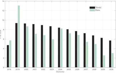
To provide further insights, we calibrate the model to the Spanish economy. The objective of the calibration is to illustrate the ability of the model to generate realistic debt profiles, and to study the qualitative and quantitative responses to unexpected income and interest rate shocks in the next section. Following Aguiar and Gopinath (2006), we set the value of the coefficient of the
2018 2019 2020 2021 2022 2023 2024 2025 2026 2027 2028 2029 2030 0
2 4 6 8 10 12 14
Figure 2.1:Maturity distribution. Data for Spain as of July 2018 and the model in the steady state.
utility function, σ, to 2, and the long-run annual risk-free rate,r∗ss, to 4 percent. We normalize income yss to 1 and the maximum maturity, T, to 20 years, as roughly 90 percent of Spanish
debt has a maturity of less than 20 years. The coupon,δ, is set to 4 percent so the market price equals one at all maturities. Steady state output is normalized to one. In order to calibrate the price impact of bonds, ¯λ, we need to set the values of the arrival rate,μ, and the spread,η, in equation (2.5). In the model, η represents the cost of capital for market makers. We calibrate this spread to 150 basis points. As a reference, we obtain an approximation of the cost of capital of the five biggest US banks in terms of their assets and compute the average spread. More details are provided in AppendixD.
We jointly calibrate the discount factor,ρ, and the arrival rate,μ, to match the average level of Spanish public debt and to replicate the average time that market makers need to exhaust bond inventories. In particular, the calibration tries to match two targets: First, the Spanish government net debt, obtained from the International Monetary FundWorld Economic Outlook
they participate in the US Treasury primary market. These two targets imply that, in the steady state,
μT
´T
0 ι(τ)dτ
=0.6, and
ˆ T
0
f(τ)dτ =0.46.
Accordingly, we set the value ofμto 0.0011 and the value ofρto 0.0416. The implied value of ¯
λ is 7.08. Note that ∂q∂ιqι ≈ ∂q∂ιψι = −12λι. We can compute the elasticity of auction prices with¯ respect to changes in the size of the issue that is produced by this calibration, to get a sense of
0 0.5 1 1.5 0
0.5 1
0 0.5 1 1.5 0.04
0.0405 0.041 0.0415
0 5 10 15 20 0
0.05 0.1 0.15 0.2
0 5 10 15 20 0
0.5 1 1.5 2
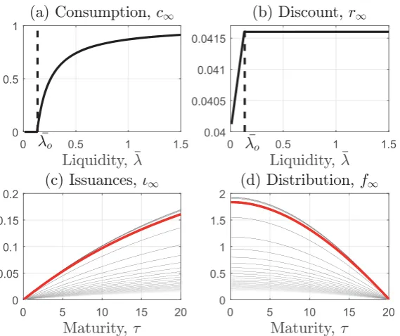
Figure 2.2: Steady-state equilibrium objects as a function of the liquidity costλ¯. Note: The thick red line in panels (c) and (d) indicates the values at the threshold ¯λo.
the magnitude of the price impact. The maximum value of issuances is 0.003, for a maturity of 20 years, and hence the elasticity of the auction price equals −12 ×7.08×0.003 = 0.011. This means that if the government duplicates the size of its steady-state issuance of the 20-year bond, the bond price falls by 1.1 percent at the time of the auction.17
Figure2.1presents the steady state debt profile generated by the calibrated model alongside the data corresponding to the Spanish debt profile of July 2018. Admittedly, the comparison has some limitations: we compare a steady state object of the model with an empirical counterpart in a particular period.18 Nevertheless, the figure shows that, despite its simplicity, the model reproduces remarkably well the decreasing maturity profile of Spanish debt. This figure
corre-17The magnitude of the price impact is roughly similar to other estimates in the literature. For instance, Faraglia
et al. (Forthcoming) consider average auction costs of 0.0028 for 10-year, 0.0026 for 9-year and 0.000284 for 1-year bonds based on the empirical findings for the US market of Lou et al. (2013). In our model, calibrated for Spain, these costs amount to 0.0065, 0.0060 and 0.00078, respectively.
18Notwithstanding, we have repeated the analysis for other periods with similar results. Results are available
sponds to outstanding amounts. We discuss the corresponding data for debt issuances in Spain between 2000 and 2018 in AppendixE.
Under the calibration, the model has a proper steady state because the calibration satisfies ¯
λ > λ¯o. Figure2.2 displays steady-state objects as functions of ¯λ. The value of the threshold ¯
λo is 0.14, well below the calibrated value of ¯λ, which is 7.08. Panels (a) and (b) show how, for
liquidity costs below the threshold, asymptotic consumptionc∞is zero because no steady state
exists. Similarly, as liquidity costs vanish, the discount factorr∞ converges to the annual risk-free rate of 4 percent. The thick red line in panels (c) and (d) indicates the values at the threshold
¯
λo. The black lines above it are the values for ¯λ ≤λ¯o. The limiting distribution is approached as ¯λ goes to zero and it is relatively similar to the distribution at the threshold. This implies that, even in the case of liquidity cost values such that no steady state exists, the asymptotic debt and issuance profiles are approximately the same as those at the threshold ¯λ =λ¯o.
2.6
Maturity management with unexpected shocks
The computation of the transitional dynamics that satisfy the analytic expressions of the solu-tion in Proposisolu-tion 1 requires a numerical algorithm. The idea follows directly from Proposisolu-tion 1: Given a guess for {c(t)}, we obtain the domestic discount factor {r(t)} through equation (2.11). This discount factor produces valuations {v(τ,t)} according to (2.10), which, in turn, determine the issuances {ι(τ,t)} through the optimal issuance rule (2.9). Issuances produce a path of debt profiles {f (τ,t)} obtained from the law of motion of debt, (2.1). Given these debt profiles and the corresponding issuance policies, the budget constraint, equation (2.2), de-termines a new consumption path. The transition to the steady state is a fixed point problem in{c(t)}, where the guess and resulting consumption paths should coincide. We present the details of this numerical algorithm in Appendix F.
We now study transitions after unexpected shocks to income or to the short-term interest rate. Transitions are initiated from a steady state debt profile. In the experiments, we reset either
y(0) orr∗(0)to an initial value, and then let the variable revert back to the steady state. Once either variable is reset, the entire path is anticipated. We study the dynamics of the debt profile. These dynamics are governed by two forces:consumption smoothingandbond-price reaction. Both forces are counterbalanced by the liquidity costs.
Consumption smoothing refers to the management of the debt profile in order to smooth consumption along a transition path. Consumption smoothing is active only when the gov-ernment is risk averse, i.e., σ > 0. This force operates even without liquidity costs, but the force has an effect on the debt maturity profile only when liquidity costs are present, ¯λ > 0.19 This force is summarized by the internal discount factorr(t) = ρ+σc˙(t)/c(t). In fact, when
r∗is constant (ψ =1), the value gap equals 1−v. In this case consumption growth shapes the maturity profile directly from the solution tovpresented in Proposition 1: if a shock produces
a growing consumption path, the domestic discount increases and the debt distribution tilts toward longer maturities, as valuations at longer horizons are affected more. The increase in domestic discounts, or equivalently the decline in domestic valuations, also induces an increase in the volume of issuances.
Bond-price reaction is a more subtle force. This force determines how the debt profile changes with bond prices, ψ(τ,t). It is present even with risk neutrality, i.e., when we shut down consumption smoothing. This force only plays a role in the presence of liquidity costs,
¯
λ > 0. Without liquidity costs, the domestic discount factor coincides with the interest rate,
r(t) = r∗(t), and since bond prices are arbitrage free, the government is indifferent between issuing at any two maturities. With liquidity costs, even a risk-neutral government is no longer indifferent. The reason is that liquidity costs allow for a gap betweenr(t)andr∗(t)as rebalanc-ing is now costly. Any gap between these two rates is compounded differently along different time horizons, and thus the government faces different consumption paths depending on its maturity choice. We can again observe how this force operates through the value gap in the simplified case of risk neutrality. In this case consumption smoothing is not active, and valu-ations are constant and equal to their steady state value vss. If a shock temporarily increases short-term rates, thereby reducing market prices−specially at long maturities, the optimal is-suance rule (2.12) prescribes a decline in debt isis-suances and a tilting of the maturity distribution toward shorter maturities. In the general case with risk aversion, interest rate shocks produce a race between consumption smoothing and bond-price reaction.
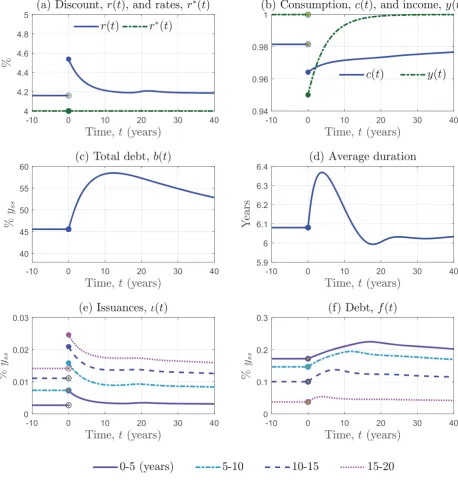
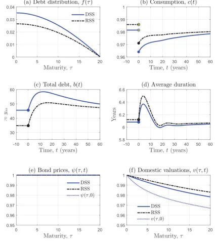
To gather further insights into these two forces, we analyze the responses to unexpected shocks to y(t) and r∗(t)separately. Consider first the response to an income shock, displayed in figure 2.3. In the experiment, income followsdy(t) = αy(yss−y(t))dt, the continuous-time counterpart of an AR(1) process. We sety(0) to a level 5 percent below its steady state value, corresponding to a major recession in Spain.20 The reversion coefficient, αy, is set to 0.2 in line with Spanish data. In this case, the only active force is consumption smoothing, as the interest rate remains constant.
Figure 2.3 displays the transition. Panels (a) and (b) show how the fall in income produces a decline in consumption on impact, followed by a recovery. The expected consumption growth produces an increase in the domestic discount on impact, which reverts back to the steady state. Since there is an increase in domestic discounting, domestic valuations decrease, which acts like a reduction in the perceived cost of debt. Given that bond prices are constant, the optimal is-suance rule (2.12) dictates an increase in the isis-suances at all maturities, as displayed in panel (e) and hence in the outstanding amount of total debt (panels c and f), b(t) ≡ ´0T f(τ,t)dτ. One noticeable feature is that new issuances are not homogeneously distributed across maturities: they are more concentrated in longer maturities, as expected. This is because long-term domes-tic valuations are more sensitive to changes in the discount factor. This produces anincreasein the average debt duration of the portfolio, computed as the average of the Macaulay duration of each individual bond (panel d).
The intuition for this pattern is the following. In response to a negative income shock, the government attempts to smooth consumption by issuing more debt. Because of the liquidity costs, the government tilts issuances toward long-term debt to minimize the liquidity costs
as-Figure 2.3: Response to an unexpected temporary drop in income.
-10 0 10 20 30 40 4
4.2 4.4 4.6 4.8 5
-10 0 10 20 30 40 0.94
0.96 0.98 1
-10 0 10 20 30 40 40
45 50 55 60
-10 0 10 20 30 40 5.9
6 6.1 6.2 6.3 6.4
-10 0 10 20 30 40 0
0.01 0.02 0.03
-10 0 10 20 30 40 0
0.1 0.2 0.3
sociated with debt rollover during the period in which the decline in income, and consumption, is more acute. The desire of the government to delay these rollover costs explains the lengthen-ing in the maturity.
ma-tures when the shock hits. In particular, the first year it issues 20-year bonds, in the second year it issues 19-year bonds, and so on (panel e). As displayed in panels (c) and (d), the government not only steadily decreases the maturity of the issuances, it also increases the amount of debt issued as the date of realization of the shock approaches. The result is a progressive build-up of
-10 0 10 20 30 40 -20
-10 0 10 20 30
-10 0 10 20 30 40 0.98
1 1.02 1.04 1.06
-10 0 10 20 30 40 42
44 46 48 50
-10 0 10 20 30 40 5.8
5.9 6 6.1 6.2
-10 0 10 20 30 40 -0.01
0 0.01 0.02
-10 0 10 20 30 40 0
0.05 0.1 0.15 0.2
Figure 2.4: Response to an unexpected drop in income 20 years ahead.
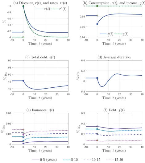
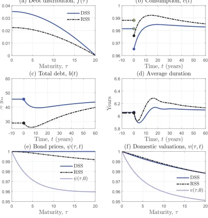
to (i) repay the principals of all the debt issued in the pre-shock period, (ii) repurchase part of its debt stock, especially at short-term maturities and (iii) increase temporarily consumption. As in the previous exercise, this strategy minimizes the liquidity costs because the government spreads out bond issuances and avoids any rollover of the extra debt prior to the shock arrival. Next, consider an unexpected shock to r∗(t), as presented in figure 2.5. We let dr∗(t) =
αr(r∗ss−r∗(t))dt, with αr = 0.2, which is also taken from the Spanish data. On impact, the
-10 0 10 20 30 40 4
4.2 4.4 4.6 4.8 5
-10 0 10 20 30 40 0.94
0.96 0.98 1
Figure 2.5: Response to an unexpected temporary shock to interest rates.
-10 0 10 20 30 40 0
0.01 0.02 0.03
-10 0 10 20 30 40 0
0.1 0.2 0.3 -10 0 10 20 30 40
40 45 50 55 60
-10 0 10 20 30 40 5.8
interest rate increases from 4 percent to 5 percent. The shock produces a consumption drop of the same magnitude as the income shock in figure 2.3, which makes both shocks comparable. In this case, both the bond-price reaction force and consumption smoothing are active.
We can interpret the transition as follows. On impact, the domestic discount jumps to 5 percent, as shown in panel (a) of figure 2.5. This narrows the value gap across all maturities. The initial effect of a narrower value gap is a decrease in all issuances (panel e). This captures the notion that, upon an interest rate increase, the government wants to sacrifice present con-sumption to mitigate a higher debt burden. A noticeable feature is that the interest rate shock produces an initial reduction in the average debt duration. This occurs even though the path of consumption resembles the one of the income shock that produces the opposite prediction
3
Risk
The previous section analyzed optimal debt-management under perfect foresight. This section presents a characterization that allows for risk. The goal is to understand how the anticipation of shocks affects the shape of the optimal debt profile and the ability to insure.
regarding debt maturity. The reason why maturity shrinks with the rate shock is that, in this case, the valuation gap decreases more for long-term bonds. The valuation gap is proxied by the interest rate gap,r(t)−r∗(t), which narrows on impact, but widens again as consumption recovers. This tells us that bond-price reaction dominates over consumption smoothing.
The intuition in this case is straightforward. Faced with temporary lower bond prices, the government decides to issue less debt. This reduction is more relevant for long-term bonds, because these are the bonds that experience the larger price declines. This effect is, neverthe-less, partially mitigated by consumption smoothing because the initial decline in consumption encourages, as discussed above, the issuance of long-term bonds.
In order to isolate the bond-price reaction force, figure H.2 in Appendix H displays the tran-sitions when the government is risk neutral, i.e, σ = 0. The effects of figure 2.5 are magnified as consumption smoothing is not active. As figure H.2 shows, once the shock arrives and bond prices fall, the government decides to directly repurchase debt, especially at long maturities, and to resell it when prices go up again. This summarizes well the essence of this force: be-cause liquidity costs make it expensive to rebalance debt across maturities, the government buys (or issues less) debt when it is temporarily cheap in order to resell it (or issue more) when prices recover.