A Case Study with Bus Trajectories
Tales P. Nogueira1, Clayson Celes2, Herv´e Martin3, Antonio A. F. Loureiro2, Rossana M. C. Andrade1 1
Group of Computer Networks, Software Engineering and Systems Federal University of Cear´a
Fortaleza, Brazil
2 Federal University of Minas Gerais
Belo Horizonte, Brazil 3 Univ. Grenoble Alpes
CNRS, Grenoble INP, LIG F-38000 Grenoble, France
{tales, rossana}@great.ufc.br, {claysonceles, loureiro}@dcc.ufmg.br, [email protected]
Abstract. The proliferation of devices with positioning capability has allowed new possibilities for studies and applications in the context of urban mobility. However, the process of analyzing raw trajectories poses several challenges. In this work, we investigate one of the main tasks in this process of trajectory analysis: detecting stops from GPS trajectories. Stops can reveal interesting behavior aspects of a moving object such as its daily routine, bottlenecks in traffic jams, or visiting times of touristic places. Although there are some efforts in this direction, most current methods ignore the presence of noise segments, which typically occur many times in trajectories. In this sense, we present a method that exploits gaps in time and space to identify episodes of movement, stop, and periods where some classification is inconclusive, which we define as noise. In addition, our method does not rely on contextual information as opposed to some current solutions, which make our proposal also suitable for trajectories recorded in free space. We compare our method to the state of the art highlighting its advantages in terms of manipulating noise, supporting spatial filtering and being independent of external resources. Moreover, we conduct an experimental evaluation using a large-scale bus dataset to show the effectiveness of our method in a real application scenario.
Categories and Subject Descriptors: H.2 [H.2.8 Database Applications]: Spatial databases and GIS; G [G.3 Prob-ability and Statistics]: Time series analysis
Keywords: outlier labeling, stop-move identification, trajectory analysis
1. INTRODUCTION
The ubiquitous presence of trajectory data is constantly growing in our digital lives and we are constantly producing it in many ways. Structuring trajectories into periods of stops and moves has been proved to be a fundamental task [Spaccapietra et al. 2008] in trajectory analysis. In fact, different criteria can be used to segment trajectories [Buchin et al. 2011; Alewijnse et al. 2014], expanding the possibilities of structuring moving object traces beyond the stop-move model. Viewing trajectories as sequences of moves and stops can be the first step towards a more complex model
This article is an extended version of Nogueira et al. [2017], presented in XVIII Brazilian Symposium on GeoInformatics (GEOINFO 2017). The authors would like to thank the French Ministry of Higher Education and Research (MESR) and the Brazilian National Council for Scientific and Technological Development (CNPq)
Antonio A. F. Loureiro has a researcher scholarship “PQ Level 1A” sponsored by CNPq. Rossana M. C. Andrade has a researcher scholarship “DT Level 2” sponsored by CNPq. This research was partially funded by INES 2.0, CNPq grant 465614/2014-0.
for trajectory analysis. Such segmentation is also important for building high-level abstractions for trajectory modelling [Nogueira et al. 2018].
Trajectories are continuous events in real life. However, they must be treated as discrete events to be recorded. Different sampling rates and optimizations can be used in this process that may hinder the ability of stop detection algorithms to correctly detect the different parts of a trajectory.
Detecting occurrence and absence of movement is a fundamental segmentation task that has been vastly explored in the literature [Alvares et al. 2007; Palma et al. 2008; Yan et al. 2010; Rocha et al. 2010; de Graaff et al. 2016]. Applications that deal with real-world data also have to deal with noisy measurements that, in some cases, make it impossible to determine the actual state of the moving object. Although some related studies have considered the presence of noise in trajectories, they usually handle this by previously smoothing or by using additional metadata that is not always available.
The characteristics of a recorded trajectory can vary broadly according to a range of factors such as sensor’s physical components, sampling rate, post-processing algorithms and environmental condi-tions. These factors may yield trajectories with different quality levels even for traces captured by the same device. Therefore, this facet of spatiotemporal data research disfavor the possibility of proposing a universal method for detecting stops and moves, as well as trajectory segmentation methods based on other criteria such as speed or direction.
In this context, a method for stop detection should consider how data is recorded and stored in order to lead to good results. Thus, it is necessary to make some assumptions about collected data before proposing a solution to the problem of trajectory segmentation.
We observe that relevant methods for identifying stops rely on the assumption that trajectories are sampled at regular time intervals. This assumption allows the application of clustering algorithms to identify points near each other and, then, classify groups of points as stops according to some temporal and spatial thresholds. However, this assumption may not hold due to a variety of reasons, such as periods of GPS failure, noisy measurements, different sampling strategies, preprocessing procedures, among other factors.
Andrienko et al. [2008] defined how a trajectory can be observed according to various sampling strategies as follows: time-based, when positions are recorded at regular time intervals;change-based, when positions are recorded only when the object moves;location-based, when the location is collected only if the object approaches a specific location, e.g., near a sensor; event-based, when the moving object performs a specific action, e.g., making a call; and various combinations of these methods. While most of the state-of-the-art methods of stop detection deal mainly with thetime-basedrecording strategy, it should be noted that some applications may store trajectories following any combination of the above types. In addition, applications may make modifications to the captured data to eliminate redundant information. In this scenario, algorithms that rely on clustering points are most likely to fail.
In this article, we describe a way of creating episodes based on the detection of stops and moves during a single trajectory. The main assumption of our method is that, for a given trajectory, points may not be sampled at the same frequency along the whole path. This may happen, for instance, in applications that apply a post-processing filter that discards points that are close to previously recorded locations or in applications that stops recording points when the object is not moving. In addition, we consider that some trajectory characteristics, namely the distance, the duration and the log of speed between consecutive points, follow an approximately normal distribution when the object is moving.
Trajectories recorded following other strategies, e.g.,time-based, can also be used with our method if redundant points points are removed based on some minimum radius criteria. It is worth to notice that this should not produce any systematic bias in the results of the method.
Another important difference in our method is that the notion of stop in other studies is usually related to the identification of Regions of Interest, allowing the classification of a point as a stop even when there is some movement. In our case, we aim at identifying locations where an actual stop happened. Moreover, our proposal does not need external data (e.g., polygons of adjacent geographic features) nor additional sensor data (e.g., GPS accuracy information). These characteristics of our proposal can be appealing for applications that deal with trajectories recorded in free space, e.g., when there are no streets or buildings nearby.
In comparison with the work of Nogueira et al. [2017], this article extends its contributions by detailing the statistical method employed by our approach, and presents an additional experiment with a large-scale bus database that shows the effectiveness of the method supported by features extracted from the OpenStreetMap (OSM) database.
The remainder of this article is organized as follows: Section 2 presents the relevant work devoted to detecting stops in trajectories. Section 3 describes characteristics of the dataset considered in this study. Section 4 explains the Outlier Labeling Rule, which is the base of our method. Section 5 details our contribution, the MSN (Move-Stop-Noise) algorithm, which is compared to other important methods in Section 6. Moreover, the solution is quantitatively evaluated with OSM data. Finally, Section 7 encloses our conclusions and perspectives of future work.
2. RELATED WORK
We can observe that many state-of-the-art stop detection methods rely on some assumptions about the gathered data and, in some cases, on additional external data as well. The SMoT method [Alvares et al. 2007] classifies as stops the trajectory points that intersect “candidate stops”, i.e., a previously defined set of polygons, each one associated with a minimum time duration. A major weakness of this approach is the need for manually selecting candidate stop polygons as well as minimal time durations needed to consider each region as a stop. Establishing a hard threshold on the duration of a stop may cause the algorithm to miss important stops that have a time duration close to but not higher than some threshold.
The SMoT method was later extended by the SMoT+ algorithm [Moreno et al. 2014]. SMoT+ is able to identify stops in different levels of granularity (e.g., a shop inside a mall located in a town). SMoT+ presents the same drawbacks of SMoT as their parameters are very similar. The concept of Interesting Sites (IS) is similar to SMoT’s candidate stops. Moreover, there is an additional parameter representing a hierarchy of containments among the sites.
The PIE algorithm [de Graaff et al. 2016] uses the underlying geography of polygons, and considers reductions in speed, changes in direction and the accuracy of each GPS point. Whereas speed and direction can be easily computed from trajectory points, the availability of accuracy data, while very important to assess signal quality, is not commonly stored by most applications. This factor imposes an important obstacle to use this method with trajectories captured by third-party applications.
Palma et al. [2008] proposed the CB-SMoT algorithm, which considers that a moving object’s speed decreases significantly when an interesting place is being visited (therefore, it is a stop). Moreover, CB-SMoT assumes that the recording device keeps storing points even when the object is not moving, thus stops are characterized as regions with a greater spatial density of points. Moreno et al. [2010] reused both SMoT and CB-SMoT to identify stops and infer the behavior of moving objects.
are smoothed and outliers are identified by using velocity thresholds according to a given domain knowledge (e.g., car, human and bicycle). In the Trajectory Structure Layer, the identification of stops is done by determining a speed threshold based on the type of the moving object and a function that takes into account the moving object’s average speed and the average speed of other moving objects. For calculating the latter, the space is divided into a grid and an average speed is associated to each cell. Differently from our proposal, the authors have used the non-robust average speed mea-sure, which may difficult a correct identification of stops if there is a large range of speeds in a single trajectory. Despite the fact that there was an effort to dynamically set speed thresholds, this was not done to the stop duration, which is still defined as an absolute metric value (e.g., 15 minutes).
Nogueira et al. [2014] proposed a statistical method for detecting candidate stops. Its only parameter is a minimum speed for a point to be considered as a stop. However, they did not consider noisy trajectory segments nor used robust statistical measures as they have relied on the standard deviation from the mean, a metric that can be easily broken by large outliers. These weaknesses are addressed in this work.
It is important to highlight that general-purpose trajectory segmentation methods can also be em-ployed to identify specific types of episodes. Soares J´unior et al. [2015] proposed GRASP-UTS, an unsupervised approach to segment trajectories with the goal of minimizing thedistortion, i.e., hav-ing the most homogeneous segments, and maximizhav-ingcompression, i.e., having the least number of segments. While the primary purpose of GRASP-UTS is not to detect stops and moves, it is com-pared to CB-SMoT with regards to purity, coverage, and the number of generated segments. More recently, the same authors have proposed a novel semantic and semi-supervised trajectory segmen-tation [Soares J´unior et al. 2018]. They fragment trajectories based on, among other features, some information previously labeled by the users, considering semantic aspects in trajectory segmentation. Whilst these approaches seem promising to segment trajectories following multiple criteria, we focus on approaches conceived explicitly for move, stop, and noise identification in this work.
3. EXPLORATORY DATA ANALYSIS
A useful task when analyzing a dataset is verifying the correlation strength among its variables. Usually, the output of this analysis highlights the relationships among variables that tend to better explain the dataset variability. In this study, we have used the Spearman correlation because it is more resistant to outliers as it diminishes the importance of extreme scores by first ranking the two variables and then correlating the ranks instead of the actual values [Myers and Well 2003].
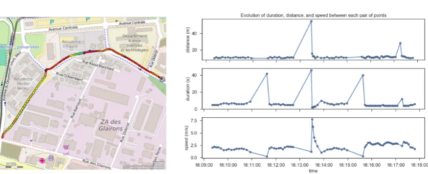
Figure 1 shows an illustrative trajectory that was recorded in a controlled manner in order to have two stops of a few seconds and two periods of noise that have been simulated by turning off the smartphone’s GPS for a few seconds.
For each pair of sequential points in the trajectory of Figure 1, we have calculated its speed, distance and duration. We can observe some interesting characteristics based on previous knowledge about this particular trajectory. The trajectory starts with distances of about 10 meters between points, durations of 5 to 7 seconds, and a fairly constant speed until there is a peak of 42 seconds in the duration between points in the dataset. At the same time, we can observe that the speed drops to a value near to zero while the distance remains unchanged. This characterizes a stop taking into consideration the characteristics of this dataset. Some seconds later, another peak in duration is noticeable at the same time of a peak in the distance between points that are not followed by a decrease in speed. This characterizes a period of noise. In the remaining of the trajectory, we can notice another stop and another noise period with these same characteristics.
Fig. 1. Example of a trajectory and its speed, distance, and duration time series
which were collected from MapMyFitness1 applications, a widely used set of mobile applications for tracking sports activities. Walking and running activities were selected. These trajectories range from 2 to 42 kilometers, are located in Grenoble (France) and Barcelona (Spain), and have been recorded with Android smartphones. Duration, distance and speed between each pair of points of each trajectory were computed. From this data, we can observe that the pairing between speed and duration is the one that presents the strongest correlation. In this case, a strong negative correlation indicates that when the values of the duration increase, the values of speed tend to decrease and vice-versa, which is what one can expect given the previously explained assumptions about the data.
Table I. Median of Spearman correlations among attributes of 2226 trajectories duration distance speed acceleration
duration 1 – – –
distance 0.16 1 – –
speed -0.86 0.29 1 –
acceleration 0.34 −0.03 −0.36 1
From this exploratory data analysis, we can conclude that there is a negative correlation between speed values and duration that characterizes a stop. For the noisy cases, there is no pair of variables that helps the classification. Thus, we make use of the assumption that points are recorded at near constant distance intervals most of the time.
4. OUTLIER LABELING RULE
Based on the exploratory data study, we can approach the classification of moves, stops and noise as an outlier detection problem. To identify outliers in time series, we use the modified z-score [Iglewicz and Hoaglin 1993]. The usage of this method is motivated by the poor performance of other popular measures like the standard deviation and the mean in the presence of outliers.
An indicator of the robustness of a statistic measure is its breakdown point, i.e., the maximum proportion of outlier data points that can be added to a dataset before the measure gives a wrong result. Themean has a breakdown point of 0% because if just one value of a given series is set to
infinity, itsmeangoes to infinity. On the other hand, themedianhas a high breakdown point because the median value of a series is only affected if more than 50% of the data is contaminated with outliers.
Another estimator that is easily modified in the presence of outliers is the standard deviation, as it takes into consideration the squared distance from the mean for each value. According to Huber and Ronchetti [2009], the most useful ancillary estimate of scale is the MAD (see Equation 1), which is the median of absolute distances from a series’ median. The constant scale factor 1.4826 makes the MAD unbiased at the normal distribution [Rousseeuw and Hubert 2011].
M AD= 1.4826×median(|Yi−Y˜|) (1)
Besides its superiority, the MAD is not yet largely used in some fields as discussed in [Leys et al. 2013], who recommend using “the median plus or minus 2.5 times the MAD method for outlier detection”. In our work, we use the modified z-score, which also uses the MAD and is based on the z-score (see Equation 2), which uses the non-robust statistics mean ( ¯Y) and standard deviation (s).
Zi= Yi−Y¯
s (2)
Iglewicz and Hoaglin [1993] recommend using the modified z-score shown in Equation 3 where each element of a series is subtracted from the median (˜x), multiplied by a factor to make the MAD consistent at the normal distribution (0.6745). As a recommendation from the authors, points having modified z-scores with an absolute value greater than 3.5 have a high probability of being outliers [NIST/SEMATECH 2012]. Another advantage of using the MAD statistic is the fact that it is also adequate for application in populations that do not fit perfectly a Gaussian distribution [Gorard 2005], which is the case for real-world GPS track datasets.
Mi=
0.6745(xi−x˜)
MAD (3)
As an example of the advantage of using MAD, consider the following set without any outlierx=
{6.27,6.34,6.25,6.31,6.28} with mean ¯x= 6.29, median ˜x= 6.28, and standard deviationσx= 0.03. Now, considering the introduction of an outlier, the set becomesx0={6.27,6.34,6.25,63.1,6.28}with mean ¯x0= 17.64, median ˜x0= 6.28, and standard deviationσ
x0 = 22.72.
We can compute the ordinary z-scores for the two sets as defined in Equation 2 and getZx={−0.6, 1.58,−1.2, 0.63, −0.31} and Zx0 ={−0.5, −0.5, −0.5, 1.99, −0.5}. Notice that using the popular threshold of 2.5 to label a value as an outlier it would not be possible to identify the outlier introduced inx0. Both sets have the sameM AD= 0.04 and if we compute the absolute distance (AD) from the median, we get the following results: ADx={0.01, 0.06, 0.03, 0.03, 0}andADx0 ={0.01, 0.06, 0.03, 56.8, 0}. Finally, applying Equation 3 to both sets yields: Mx ={−0.22, 1.34, −0.67, 0.67, 0} and Mx0 = {−0.22, 1.34, −0.67, 1277, 0}. In this case, the outlier in the second set highly exceeds the recommended threshold of 3.5.
5. THE MSN ALGORITHM
Our statistical method for stop, move, and noise (MSN) detection builds upon the previously explained theoretical background.
For each pair of points{(si, ti),(si+1, ti+1)}, we compute its distance, duration, speed, and turning angle. Then, we store these values in their respective time seriesSτ, Tτ, Vτ, Aτ. For Aτ, a turning angle consists on the angle formed by three neighboring points.
From the above time series, we can formulate an algorithm to determine which instants of the trajectory are likely to be stops, moves or undefined states, considered as noise in this work (see Algorithm 1). The algorithm’s inputs are the initial calculated time series besides the thresholdss, t, and v representing the modified z-score limits for distance, duration, and speed. Additionally, a minimum turning angle parameter (θ) can be used to improve the noise detection following the intuition that it is improbable for a moving object to take successive turns with small angles, and a random uniform jitter (ρ) to avoid the MAD breakdown point. Theρparameter defines the lower and upper boundaries of an interval from where some value will be randomly selected and added to the duration value of each point. It should be set to a low value (e.g., 0.5) to change the original values minimally.
As the trajectory sampling rate is assumed to be nearly constant while the object is moving and locations are not recorded while the object is stopped, the problem can be summarized as searching for outliers into time series as they are expected to have relevant gaps in time that characterize periods of stop or noise. These gaps in time coincide with decreases in speed for the cases of stops as can be observed by the negative correlation between these two variables (Table I).
To better explain the MSN algorithm, we consider the example of a trajectory depicted in Figure 1 with the following parameters: s=v= 3.5,t= 5.0,θ= 45. It is important to notice that we have used the recommended threshold of 3.5 for both distance (s) and speed (v) parameters. However, for the duration threshold (t), we have achieved better results when we increased it to 5.0 as some slow walking segments were being misclassified as stops.
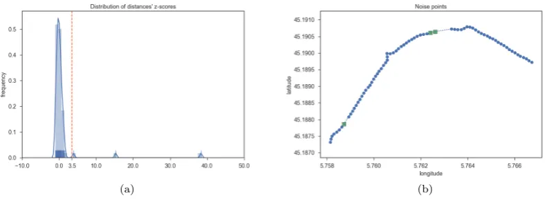
The first part of MSN identifies potential noisy points. This classification, shown in Lines 2–8, identifies points with relatively long distances. In the example (Figure 5), three points are identified in this case. They have distances of about 17, 28, and 55 meters, while the median distance of all pairs of sequential trajectory points is 11 meters.
(a) (b)
Fig. 2. The density plot of distances in (a) and the three trajectory points with long distances in (b)
Algorithm 1Move-Stop-Noise classification algorithm
1: procedureMoveStopNoise(Sτ, Tτ, Vτ, Aτ, s, t, v, θ, ρ)
2: distance outliers ←[ ]
3: Ms←ModifiedZScore(Sτ, M ADs,s˜) .Equation 3 4: fori←0tolength(Ms)do:
5: if Ms[i]> sthen .Identifying long distances
6: Append itodistance outliers 7: end if
8: end for
9: direction outliers ←[ ]
10: fori←0tolength(Aτ)do:
11: if Aτ[i]< θandAτ[i+ 1]< θ then . Identifying sharp turning angles 12: Append iandi+ 1 todirection outliers
13: i++
14: end if 15: end for
16: noise indexes ←distance outliers +direction outliers
17: clean indexes ←τ−τ[noise indexes]
18: τ ←τ[clean indexes] . Removing noisy points
19: Tτ ←Tτ+ρ .Adding a random uniform jitter
20: duration outliers ←[ ]
21: Mt←ModifiedZScore(Tτ, M ADt,˜t) 22: fori←0tolength(Mt)do:
23: if Mt[i]> tthen . Identifying long durations
24: Append itoduration outliers
25: end if 26: end for
27: Vτ ←lnVτ . Natural log of speed
28: speed outliers ←[ ]
29: Mv←ModifiedZScore(Vτ, M ADv,v˜) 30: fori←0tolength(Mv)do:
31: if Mv[i]<−v then . Identifying slow speeds
32: Append itospeed outliers
33: end if 34: end for
35: stop indexes ←duration outliers T speed outliers
36: move indexes ←clean indexes −stop indexes
37: returnmove indexes,stop indexes,noise indexes 38: end procedure
Once a potential noise is identified, the second part of our method consists in labeling potential stops, but before that, the noise points are removed for the further analysis.
Then, the modified z-score is applied to find duration gaps. However, we have set the modified z-score threshold to 5 to avoid false positives. Figure 3 shows the distribution of durations for the example. Two long durations with 40 and 42 seconds are identified, while the median duration for the trajectory is 5 seconds.
Fig. 3. Distribution plot of a slightly “jittered” duration between points with two outliers
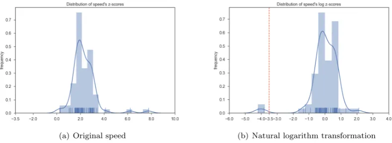
The complement of stop identification (Lines 27–34) concerns the analysis of speed time series. The Outlier Labeling Rule, presented in Section 4, should be applied to approximately normally distributed datasets. However, for the trajectories considered in this work, speed data has demonstrated to be positively skewed in general. To normalize the speed data, the natural logarithm was applied to restore symmetry. Figure 4 shows the importance of this transformation to find slow speed outliers. In Figure 4(b), it is possible to see that two points have speeds relatively slower (0.23m/sand 0.29m/s) while the median speed value for the sample trajectory is 2.1m/s.
(a) Original speed (b) Natural logarithm transformation
Fig. 4. Difference of speed data before and after natural logarithmic transformation. The outlier threshold is shown in (b)
of the stop greater than normal. On the other hand, due to the accuracy of GPS acquired positions, the sequence may actually represent a period where the object was stationary. A possible approach for these cases could involve analyzing more variables. For instance, one could define a threshold to the number of contiguous points with low speed where sequences having more points than the threshold are considered as moves. We left this task as a future work.
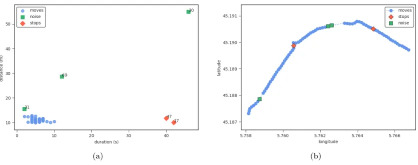
Finally, we classify points that present both slow speed and long durations as stops. Figure 5 shows these two variables with their respective thresholds. Figure 6 shows all points with their classification as either move, stop, or noise. According to our algorithm, points located at the lower right corner in Figure 6(a) are stops.
Fig. 5. Modified z-scores of speed and duration with their thresholds. Points classified as noise have been removed in this figure
(a) (b)
6. EVALUATION
In this section, we evaluate MSN in two perspectives. First, we focus on qualitatively analyzing the performance of the MSN algorithm over other stop classification methods. Second, we conduct a set of experiments to evaluate the accuracy of the MSN algorithm in a real application scenario.
6.1 Qualitative Evaluation
Due to the assumptions about trajectory sampling strategies, it is difficult to make a comparison with the related work by running all algorithms with the same set of trajectories. In this evaluation, we focus on analyzing the theoretical performance of other stop classification methods and highlight the main differences from our work.
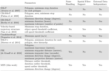
Table II shows a general comparison of the main algorithms for stop detection in the literature. As advantages of our method, we can point out the independence of external data, the usage of characteristics that can be completely extracted from the trajectory points, the robustness of statistic methods involved, and the handling of noise.
Table II. Comparison of stop detection algorithms
Parameters Noise Handling Spatial Filter Support External Data Independence SMoT
[Alvares et al. 2007]
Polygons, minimum stop duration
for each polygon No No No
CB-SMoT [Palma et al. 2008]
Polygons, area, minimum stop
duration No No No
DB-SMoT [Rocha et al. 2010]
Minimum direction change (degrees), minimum duration (hours),
maximum tolerance (number of points)
No No Yes
Velocity-based trajectory structure [Yan et al. 2010]
Minimum stop duration,
object speed threshold coefficient, cell speed threshold coefficient
No Yes No
CandidateStops
[Nogueira et al. 2014] Minimum speed (m/s) No Yes Yes
SMoT+
[Moreno et al. 2014]
Polygons, minimum duration for each
polygon, sites hierarchy No No No
PIE
[de Graaff et al. 2016]
Polygons,
maximum inaccuracy (meters), minimum staypoint distance (meters), minimum staypoint time (seconds), minimum direction change (degrees), maximum projection distance (meters)
Yes No No
MSN (this work)
Distance outlier threshold, duration outlier threshold, speed outlier threshold,
minimum direction change (degrees)
Yes Yes Yes
By not relying on the polygons of the underlying geography, our method is adequate to trajectories that are not in a constrained space, being able to identify stops also in free space. In addition, apart from the minimum turning angle in degrees, an important aspect of MSN is that the other threshold parameters are not based on any metric quantities, e.g., distance in meters or duration in seconds. Instead, the Outlier Labeling Rule allows the usage of more abstract thresholds.
method on outlier detection for approximately normally distributed data. However, if the trajectory contains a large number of noise episodes and, therefore, large time gaps, the method may fail in recognizing stops. A possible strategy to mitigate this consists in running MSN once and analyzing the retrieved noise episodes. Then, one could apply some preprocessing procedure (e.g., interpolation) to smooth out the noisy segments [Celes et al. 2017] and rerun the algorithm. In this process, it is also possible to conclude that the quantity of erroneous data makes further analysis unfeasible.
The MSN method can be implemented inO(n+m) considering a raw trajectory withnpoints before noise removal and mpoints after the noise identification step. In the worst case, n=m(no points are discarded in the noise classification phase). Thus, the algorithm’s complexity isO(2n) =O(n), which continues to be linear. For the sake of clarity, we have not shown the most concise and efficient implementation of MSN in Algorithm 1, but it could be easily refactored as a singlefor loop.
6.2 Quantitative Evaluation
In this evaluation, we present experiments with the Dublin Bus GPS sample data from Dublin City Council2. The trajectories were collected from Nov 6, 2012 to Nov 30, 2012 and gather data from buses that run the lines of Dublin’s public transport. In this dataset, trajectories can be isolated by grouping pairs of vehicle journeys and lines, totaling 251,006 traces.
Despite the huge volume of trajectory data, we observed that some traces had features that would difficult the application of our method. Therefore, some preprocessing and filtering steps were neces-sary to select a subset that matched some quality criteria.
Some of the trajectories had points recorded at exactly the same position. This goes against MSN’s assumption of spatial filtering, i.e., points are only recorded if the moving object is distant by a given amount of space from its last recorded position. To correct this, we dropped points recorded at the same location while keeping only the first one as a first preprocessing step.
Second, we computed the standard deviation of the distance between points for each trajectory. This measure gives an estimation of how sparse or concentrated the points are, and allowed us to filter trajectories that had a better distribution of points along the entire route. Three criteria were used to select the sample data for the experiments: (i) the standard deviation of the distance between points should be less or equal to 60 meters; (ii) the trajectories should have at least 80 points; and (iii) the duration of travels should be 200 minutes of less.
After the preprocessing step, we performed a characterization to describe the features of the Dublin Bus GPS sample data. The data used in this work consists of 1,574 trajectories from different buses from Dublin’s public transport that were select according to the preprocessing criteria explained above.
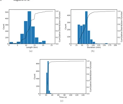
Figure 7 shows the main aspects in terms of spatial and temporal features of that sample data. The length of the selected trajectories, depicted in Figure 7(a), varies from a few meters to about 26 kilometers. Approximately 75% of the selected trajectories have a length smaller than 15km, as expected in bus mobility scenarios. Some trajectories have a length greater than 15km representing some bus lines crossing the city. Naturally, the duration of the displacement of each trajectory is related to its length, as can be seen in Figure 7(b), where we can observe that most of the trajectories have between 25 and 75 minutes of duration. Moreover, we observe the time between two consecutive points in each trajectory. Figure 7(c) shows that approximately 75% of the selected trajectories have average time between two consecutive points smaller than 26 seconds, as observed in the whole dataset.
Once the sample trajectories were selected, we run the MSN algorithm with each one of them. Then, for each detected stop, we queried the OSM database to verify which features were located around the stop position. To consider the uncertainty inherent to GPS recordings, we considered a radius of
0 5 10 15 20 25 Length (km) 0 100 200 300 400 500 Co un t 0.0 0.2 0.4 0.6 0.8 1.0 Cu mu lat ive D ist rib uti on Fu nc tio n (a)
0 25 50 75 100 125 150 175 200 Duration (min) 0 100 200 300 400 Co un t 0.0 0.2 0.4 0.6 0.8 1.0 Cu mu lat ive D ist rib uti on Fu nc tio n (b)
0 20 40 60 80 100 120 140 Time (s) 0 200 400 600 800 Co un t 0.0 0.2 0.4 0.6 0.8 1.0 Cu mu lat ive D ist rib uti on Fu nc tio n (c)
Fig. 7. Characterization of the trajectories from Dublin Bus GPS sample data: (a) Size of the trajectories; (b) Duration of the trajectories; (c) Average period between two adjacent GPS points
50 meters around the stops and retrieved only OSM features that held tags containing “highway” as key3, which serves to describe roads, streets, paths, and the features along them.
Next, we excluded highway features tagged with the following values as these are not related to stops: street lamp, street cabinet, city junction, elevator, speed camera, and milestone. It is worth noticing that far more values can be associated with the highway key in OSM. This exclusion subset was created based on a manual analysis of the features near stops identified by MSN in this specific sample dataset. The following tag values were considered as relevant in this work: traffic signals,bus stop,crossing,stop,turning circle,mini roundabout, andgive way.
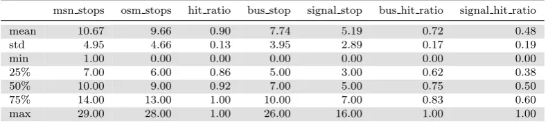
Table III shows results of the experiment for the Dublin Bus sample dataset. When we compare the values of stops detected by the MSN method (column msn stops) with the OSM stops (column osm stops), we can see that the hit ratio is equal to 90%. In other words, it shows that 90% of stops were detected near a OSM feature related to a stop. Possibly, the MSN method detected more stops than the OSM features due to inherent factors of the mobility of urban buses such as driver behavior, stops in places not previously defined, and so on. Moreover, 72% of these stops detected by the MSN method are located next to bus stops and 48% of them are not far from traffic signals. It is also important to notice that, for the second half of the dataset, the success ratio is over 92%, reaching 100% for at least 25% of the trajectories (75thpercentile).
Table III. Results for the Dublin Bus sample dataset
msn stops osm stops hit ratio bus stop signal stop bus hit ratio signal hit ratio
mean 10.67 9.66 0.90 7.74 5.19 0.72 0.48
std 4.95 4.66 0.13 3.95 2.89 0.17 0.19
min 1.00 0.00 0.00 0.00 0.00 0.00 0.00
25% 7.00 6.00 0.86 5.00 3.00 0.62 0.38
50% 10.00 9.00 0.92 7.00 5.00 0.75 0.50
75% 14.00 13.00 1.00 10.00 7.00 0.83 0.60
max 29.00 28.00 1.00 26.00 16.00 1.00 1.00
As a threat to the validity, it should be taken into consideration that some of the OSM bus stops matched to the MSN stops may not be the ones of the corresponding bus lines where the buses are supposed to stop. Due to the radius considered in the experiments, the matched features may be even in different streets outside the bus line, e.g., in parallel streets or crossings. A possible solution to this problem would consist in using GTFS (General Transit Feed Specification)4 information where the actual stop locations and times could be considered as ground truth. For the sample dataset used in this work, GTFS data for the corresponding period was not found.
7. CONCLUSION
In this work, we have proposed a new algorithm for detecting episodes of movement, stop, and noise in trajectories called MSN and evaluated its efficiency with a large-scale real dataset. This method is tailored for trajectories that have been sampled at irregular intervals of time or have been preprocessed to eliminate redundant points at near locations. This particular characteristic present in some datasets violates a basic assumption made by state-of-the-art methods, which rely on clustering nearby points, and have motivated our work to fill this gap.
The MSN method has also been designed to be independent of external data (e.g., the underlying geographic features), which render it as a viable option for trajectories recorded in free-space or lacking contextual data. Moreover, the main parameters of MSN are expressed in no particular system of measurement, i.e., there is no need for defining hard thresholds such as specifying that each stop has to have a duration equal or greater than 10 seconds, for instance. Conversely, the parameters used in our method are informed as absolute numbers as proposed by a robust outlier detection method that can be adapted if needed by the application. This is an important aspect that our work offers to advance the spatiotemporal analysis field in the area of stop detection methods.
As future work, we envision the application of other algorithms, notably supervised learning ones, as the algorithm proposed in this article takes advantage only of statistical properties of individual trajectories. Training data is important to apply a supervised approach that implies a manually annotated trajectory dataset with known labels. Therefore, a tool to annotate trajectories with stops and moves can be an interesting development. This may improve results by specializing the algorithms for heterogeneous scenarios where different devices capture positional data using their own sampling strategies and post-processing procedures. Moreover, a labeled dataset would be useful for evaluating the efficiency and accuracy of MSN. For public transportation datasets, using GTFS data is another way of achieving this improvement.
In addition, we believe that the MSN method plays a key role in several applications that explore trajectories in the context of urban mobility. In this sense, we aim to extend the MSN method to consider trajectories of several entities instead of individual trajectories. In this way, we can detect situations that happen collectively such as congestion and collective mobility routines.
REFERENCES
Alewijnse, S. P. A.,Buchin, K.,Buchin, M.,K¨olzsch, A.,Kruckenberg, H.,and Westenberg, M. A. A Frame-work for Trajectory Segmentation by Stable Criteria. InProceedings of the 22nd ACM SIGSPATIAL International Conference on Advances in Geographic Information Systems. New York, USA, pp. 351–360, 2014.
Alvares, L. O.,Bogorny, V.,Kuijpers, B.,de Macedo, J. A. F.,Moelans, B.,and Vaisman, A.A Model for En-riching Trajectories with Semantic Geographical Information. InProceedings of the 15th Annual ACM International Symposium on Advances in Geographic Information Systems. New York, USA, pp. 22:1–22:8, 2007.
Andrienko, N.,Andrienko, G.,Pelekis, N.,and Spaccapietra, S. pp. 15–38. In F. Giannotti and D. Pedreschi (Eds.),Basic Concepts of Movement Data. Berlin, Heidelberg, pp. 15–38, 2008.
Buchin, M.,Driemel, A.,van Kreveld, M.,and Sacristan, V. Segmenting Trajectories: A Framework and Algo-rithms Using Spatiotemporal Criteria.Journal of Spatial Information Science (3): 33–63, 2011.
Celes, C., Silva, F. A.,Boukerche, A., Andrade, R. M. d. C., and Loureiro, A. A. F. Improving VANET Simulation with Calibrated Vehicular Mobility Traces. IEEE Transactions on Mobile Computing 16 (12): 3376– 3389, 2017.
de Graaff, V.,de By, R. A.,and van Keulen, M.Automated Semantic Trajectory Annotation with Indoor Point-of-interest Visits in Urban Areas. In31st Annual ACM Symposium on Applied Computing. Pisa, Italy, pp. 552–559, 2016.
Gorard, S. Revisiting a 90-year-old debate: The advantages of the mean deviation. British Journal of Educational Studies53 (4): 417–430, 2005.
Huber, P. J. and Ronchetti, E. M.Robust Statistics. Wiley Series in Probability and Statistics. John Wiley & Sons, Inc., Hoboken, NJ, USA, 2009.
Iglewicz, B. and Hoaglin, D. C. Volume 16: How to Detect and Handle Outliers. InThe ASQC Basic References in Quality Control: Statistical Techniques, E. F. Mykytka (Ed.). ASQC/Quality Press, pp. 87, 1993.
Leys, C.,Ley, C.,Klein, O.,Bernard, P.,and Licata, L.Detecting outliers: Do not use standard deviation around the mean, use absolute deviation around the median. Journal of Experimental Social Psychology49 (4): 764–766, 2013.
Moreno, B.,Times, V. C.,Renso, C.,and Bogorny, V.Looking Inside the Stops of Trajectories of Moving Objects. InXI Brazilian Symposium on Geoinformatics. Campos do Jord˜ao, Brazil, pp. 9–20, 2010.
Moreno, F.,Pineda, A.,Fileto, R.,and Bogorny, V. SMOT+: Extending the SMOT algorithm for discovering stops in nested sites.Computing and Informatics33 (2): 327–342, 2014.
Myers, J. L. and Well, A. D. Research Design and Statistical Analysis. Lawrence Erlbaum Associates, Mahwah, USA, 2003.
NIST/SEMATECH. NIST/SEMATECH e-Handbook of Statistical Methods, 2012.
Nogueira, T. P.,Andrade, R. M. C.,and Martin, H. A Statistical Method for Detecting Move, Stop, and Noise Episodes in Trajectories. InVXIII Brazilian Symposium on Geoinformatics. Salvador, Brazil, pp. 210–221, 2017. Nogueira, T. P.,Braga, R. B.,de Oliveira, C. T.,and Martin, H. FrameSTEP: A framework for annotating
semantic trajectories based on episodes.Expert Systems with Applicationsvol. 92, pp. 533 – 545, 2018.
Nogueira, T. P.,Braga, R. B.,and Martin, H. An Ontology-Based Approach to Represent Trajectory Character-istics. In5th International Conference on Computing for Geospatial Research and Application. Washington, DC, USA, pp. 102–107, 2014.
Palma, A. T.,Bogorny, V.,Kuijpers, B.,and Alvares, L. O. A Clustering-based Approach for Discovering Inter-esting Places in Trajectories. In23rd Annual ACM Symposium on Applied Computing. New York, USA, pp. 863–868, 2008.
Rocha, J. A. M. R.,Times, V. C.,Oliveira, G.,Alvares, L. O.,and Bogorny, V. DB-SMoT: A direction-based spatio-temporal clustering method. In5th IEEE International Conference Intelligent Systems. London, UK, pp. 114–119, 2010.
Rousseeuw, P. J. and Hubert, M. Robust statistics for outlier detection. Wiley Interdisciplinary Reviews: Data Mining and Knowledge Discovery1 (1): 73–79, 2011.
Soares J´unior, A.,Moreno, B. N.,Times, V. C.,Matwin, S.,and Cabral, L. A. F. GRASP-UTS: An algorithm for unsupervised trajectory segmentation.International Journal of Geographical Information Science29 (1): 46–68, 2015.
Soares J´unior, A.,Times, V. C.,Renso, C.,Matwin, S.,and Cabral, L. A. F. A Semi-Supervised Approach for the Semantic Segmentation of Trajectories. In19th IEEE International Conference on Mobile Data Management. Aalborg, Denmark, pp. 145–154, 2018.
Spaccapietra, S.,Parent, C.,Damiani, M. L.,Macedo, J. A. F.,Porto, F.,and Vangenot, C. A Conceptual View on Trajectories.Data & Knowledge Engineering65 (1): 126–146, 2008.