Bayesian Estimators for Normal Distribution Parameters, the
Frequentist and Bayesian Approaches in Inferential Analysis
Klodiana Bani, Markela Muca
(Department of Applied Mathematics, Faculty of Natural Sciences, University of Tirana)
---
************************
---Abstract:
The three goals of the inferential analysis are: parameter estimation, prediction from data and the model comparison. Usually a parameter of a probability distribution is unknown but determines the property of the distribution, that in the case of the normal distribution are its mean and standard deviation. The “bell curve” of the normal distribution is totally defined by the mean which is its centre and the standard deviation which is its width. For the prediction it is needed the estimation of certain parameters to predict future data. Moreover, the comparison of the models it is related with the selection of the best model among two or more suitable models which explain the data.
The Frequentist inference is based on the long term frequencies but the Bayesian inference is mostly related to the degrees of belief and logical support. Shortly, the overview of the Frequentist means that probabilities are equal to the long term frequencies of an event without attaching them to hypothesis or to any fixed but unknown values, but in contrast with this, for a Bayesian it is possible to use probabilities to represent uncertainty or hypothesis.
In this article, it will be presented the estimation of the normal distribution parameters from the Bayesian inference and at least it will be discussed the comparison of the estimators from the classical and Bayesian analysis from the results obtained from simulations.
Keywords —Normal distribution, prior distribution, posterior distribution, Bayesian analysis.
---
************************
---I. INTRODUCTION
It was reverend Thomas Bayes who proposed Bayesian theory in 1763 and used it for the quantification of binomial distribution by the collected data. Then was Laplace who discovered and named it in 1812 in a generalised form for solving various problems.
Despite its applications, for more than 100 years, the degree of credibility of Bayesian analysis was rejected as vague and subjective and frequencies were accepted only by statisticians.
It was Jeffreys in 1939 ([1]) who rediscovered it and built the modern Bayesian theory in 1961. It was then that the two schools of statistics: Bayesian
and Frequentists were distinctly different and set apart. By the 1980s it still remained limited to use due to the needs in the calculations.
Since 1990, it became practical thanks to the rapid developments of hardware and software. The Bayesian techniques, in this way, were applied in various fields of science such as economics, medicine, biology, engineering and so on.
A random variable has normal distribution with expectation θ and variance σ2 when it distribution is given by formula (1):
, 2
1 ) , |
( 2
2
) ( 2 1
2 σ
θ
σ π σ
θ
− − =
y e y
p y∈R (1)
This distribution has several important features:
• It is symmetrical according to parameterθ
and themode, median and mean is θ. • About 95% of the population lies within
the range (-1.96σ, 1.96σ).
• The linear combination of random variables with normal densities is also a random variable with normal density. This means that if X ~N(µ,r2) and Y~N(θ,σ2) then aX+bY~N(aµ+bθ, a2r2+b2σ2).
• The most useful commands in language R for generating normal distribution are:
dnorm, rnorm, pnorm, qnorm.
II. INFERENTIAL ANALYSIS FOR THE MEAN AND THE CONDITIONING WITH THE VARIANCE
Suppose that we have Y1, Y2,…,Yn indipendent
random variables identically distributed with normal distribution N(θ,σ2). The sample distribution is given by the formula:
− − = = = =
∑
∏
∏
= − − − = = 2 1 2 2 ) ( 2 1 1 2 1 2 1 2 1 exp ) 2 ( 2 1 ) , | ( ) , | ,..., ( 2 2 n i i n y n i i n i n y e y p y y p i σ θ πσ σ π σ θ σ θ σ θBy splitting the quadratic form under the exponent, it can be seen that p(y1,...,yn|θ,σ2) depends on y1, y2, …, yn :
2 2 1 2 1 2 2 2 1 2 1
σ
θ
σ
θ
σ
σ
θ
n y y y n i i n i i n ii = − +
−
∑
∑
∑
= = = .From this equation it can be shown that the
two-dimensional statistics (
∑
= n i i y 1 ,
∑
= n i i y 1 2) is a sufficient
statistic for the pair of parameters (θ, σ2), from
which it derives that the statistics (
∑
= = n i i y n y 1 1 ,
∑
= − − = n i i y y n s 1 2 2 ) ( 1 1) is a sufficient
two-dimensional statistic for (θ, σ2).
The inferential analysis for this bi-parametric model can be divided into two separate parametric problems. According to Carlin ([4]), prior
distributions can be built in different ways, mainly from a given value. Let’ s first assume that we want to estimate θ when σ2 is known and for θ will be used a conjugate prior distribution, considering that a prior distribution family is called conjugate if for a given sample the posterior distribution is in the same family of distribution ([10]). For each prior distribution p(θ|σ2), the posterior distribution will satisfy the equation (2):
2 2 1 1 2 2 ) ( 2 ) ( 2 1 2 2 1 ) | ( ) | ( ) , ,..., | ( c c y n e p e p y y p n i i − − − × ∝ ∑ × ∝ = θ θ σ σ θ σ θ σ
θ (2)
From the equation, we have p(θ|σ2) to be
conjugate then it must contain the quadratic term
2 2 1( c )
c
e θ− . The simplest family of probability
distributions in R that fulfills this condition is the family of normal distributions, which means that if
p(θ|σ2) is a normal distribution and we consider the sample y1, y2,…,yn from this distribution then
) , ,..., |
(θ y1 yn σ2
p is also normal. Assuming that
θ~N(µ0,τ02) then the equations are true:
− − × − − ∝ ∝ =
∑
= 2 1 2 2 0 2 0 2 1 2 2 1 2 1 2 2 1 ) ( 2 1 exp ) ( 2 1 exp ) , | ,..., ( ) | ( ) | ,..., ( / ) , | ,..., ( ) | ( ) , ,..., | ( θ σ µ θ τ σ θ σ θ σ σ θ σ θ σ θ i n i n n n n y y y p p y y p y y p p y y pAdding the exponents and not considering -1/2, we have: c b a n y y n i i n i i + − = + − + + −
∑
∑
= = θ θ θ θ σ µ θµ θ τ 2 ) 2 ( 1 ) 2 ( 1 2 2 1 1 2 2 2 0 0 2 2 0where 2 2
0 1
σ τ
n
a= + , 12
2 0 0 σ τ µ
∑
= + = n i i yb and
) ,..., , , ,
( 0 02 2 y1 yn c
c= µ τ σ .
Let we show that ( | ,..., , 2)
1 σ
θ y yn
p has the
{
}
− − =
− −
∝
+ +
− −
=
− ∝
2 2
2 2
2 2
2 2
1
/ 1
/ 2
1 exp )
/ ( 2 1 exp
/ 2 1 ) / /
2 ( 2 1 exp
2 exp
) , ,..., | (
a a b a
b a
a b a
b a b a
b a
y y
p n
θ θ
θ θ
θ θ
σ θ
The function has exactly the same graphical shape with the normal distribution curve where
a /
1 is playing the role of standard deviation and b/a is the expectation value. While a probability distribution is determined by the shape of its curve, then p(θ| y1,...,yn,σ2) is a normal distribution. Marking with µn and τn2 the posterior distribution
parameters then:
2 2 0 2
1 1 1
σ τ τ
n a
n
+ =
= ,
2 2 0
2 0 2 0
1 1
σ τ
σ µ τ µ
n y n
a b n
+ + =
= .
A. The Combination of Information
Conditional probability distributions of parameters µn andτn2 are obtained as a combination
of parameters µ0 and τ02 with the sample elements.
From the variance of the posterior distribution it results that 2 2
0 2
1 1
σ τ τ
n
n
+
= which means the inverse variance of the prior distribution is obtained from the inverse variance of the sample. The inverse variance is called accuracy of the model, so we have:
• σ~2 =1/σ2 = accuracy of the sample(it shows how near is yi with parameter θ)
• 2
0 2 0 1/
~ τ
τ = = accuracy of prior distribution • ~2 1/ 2
n
n τ
τ = = accuracy of posterior distribution
It is reasonable to see the accuracy as additional information about the model:
2 2
0
2 ~ ~
~ τ σ
τn = +n ⇔
(posterior information= prior information+ sample information)
The mean of posterior distribution is given by the formula (3):
y n n
n
n 2 2
0 2
0 2 2 0
2 0
~ ~
~ ~
~ ~
σ τ
σ µ
σ τ
τ µ
+ + +
= (3)
Thus, the mean of the posterior distribution is measured from mean of the prior distribution and sample mean. The weight of the sample mean is n/σ2which is also the accuracy of the sample mean, also the weight of the prior distribution 2
0 /
1 τ serves as the accuracy of the prior distribution. If the mean of prior distribution is based on observations by the same population Y1, Y2,…,Yn then the variance of
the mean of prior observations is τ02=σ2/k0. In this way the mean of the posterior distribution is written:
y n k
n
n k
k
n
+ + + =
0 0 0
0
µ
µ
.B. The Prediction
We will consider the prediction of a new observation by a population after we have made the observations (Y1=y1, Y2=y2, …, Yn =yn) and we must
find the distribution for prediction. It is true that:
{
2}
, | ~
σ θ
Y ~N(θ,σ2)⇔Y~=θ+ε~,
{
2}
, | ~
θ
σ
ε
~N(0,σ
2).In other words, accepting that Y~has a normal distribution with expectation θ is the same thing as saying that it is given a sum of θ with a normal distributed noise which expectation is 0. Using this result, we can first calculate the mean of the posterior distribution and the variance of:
• E(Y~|y1,y2,...,yn,σ2)=E(θ+ε~|y1,y2,...,yn,σ2)
n n
n
n E y y y
y y y E
µ
µ
σ
ε
σ
θ
= + =
+ =
0
) , ,..., , | ~ ( ) , ,..., , |
( 2
2 1 2
2 1
• (~| , ,..., , ) ( ~| , ,..., , 2)
2 1 2
2
1 y yn
σ
Dθ
ε
y y ynσ
y Y
D = +
2 2
2 2
1 2
2
1 | , ,..., , )
~ ( ) , ,..., , | (
σ
τ
σ
ε
σ
θ
+ =
+ =
n
n
n D y y y
y y y D
Since the sum of normal independent variables with normal distributions is also normal then
ε
θ
~~
+ =
Y has a normal distribution.
Thus, the predictive distribution is as in (4):
{
2}
2
1, ,..., ,
| ~
σ
ny y y
Y ~N(
µ
n,τ
n2 +σ
2) (4)As an illustration, we will use simulated data with a small sample size from a normal distribution which mean is 1.8. This is the prior information to be used for the calculations of the parameters for prior and posterior distribution of mean and variance respectively. So, we have nine simulated values from the normal distribution N (1.8, 0.015):
1.638164, 1.663346, 1.812662, 1.629400, 1.705748, 1.820818, 1.659060, 1.912620, 1.777257
The population mean is taken µ0=1.8 and for the
variance we suppose that the greater part of probability lies between the double of standard deviation from the sample mean, that is µ0-2 τ0>0 or
τ0<1.8/2=0.90. The results are shown in Table 1 for each distribution of the population mean:
TABLE1 RESULTS OF THE PARAMETERS
Parameters Sample Prior Posterior
Mean 1.735 1.8 1.742
Variance 0.01 0.81 0.01
If σ2=s2=0.01 then
{
θ| y1,y2,...,yn,σ2 =0.01}
~ )01 . 0 , 742 . 1 (
N .
Fig. 1 The prior and the posterior distribution of the population mean.
In the Fig. 1 are shown with the red line the prior distribution and with the blue line the posterior distribution for population mean.
III. INFERENTIAL ANALYSIS OF THE UNKNOWN
MEAN AND UNKNOWN VARIANCE
Bayesian inferential analysis for two or more parameters is not very different in the concept of the one with one parameter. For the joint prior distribution p(θ,σ2) of the parameters θ and σ2, the
finding of the posterior distribution is related to the use of the Bayes rule where usually the conditional distribution can be substituted by the maximum likelihood function ([5]):
) ,..., , (
) , ( ) , | ,..., , ( ) ,..., , | , (
2 1
2 2
2 1 2
1 2
n n n
y y y p
p y
y y p y y y
pθ σ = θ σ θ σ
The procedure begins by finding a family of conjugate prior distributions that makes easy the calculation of posterior distribution. Starting from the conditional probability formula, we get the multiplication formulas and so the joint distribution is written:
) ( ) | ( ) ,
(
θ
σ
2 pθ
σ
2 pσ
2p =
We showed earlier that when σ2 was known, a prior distribution for θ is the normal distribution (µ0,
τ02). Consider the special occasion when
0 2 2
0 σ k
τ = :
) ( ) / ,
, (
) ( ) | ( ) , (
2 0
0 0
2 2 2
σ σ
τ µ θ
σ σ θ σ
θ
p k dnorm
p p
p
× =
=
=
In this case, the parameters µ0 and k0 can be
interpreted as the mean and the sample size of sample from a previous observation set. For σ2 we need a prior distribution family to be positively defined in (0, ∞). Such a distribution family is the family of gamma distributions, but unfortunately this distribution family is not conjugate for the variance of a normal variable. However, the family of gamma distributions is conjugate to 1/ σ2 (the accuracy of σ2). When it is used such a prior distribution, it is said that σ2 has a gamma inverse distribution:
accuracy=1/ σ2~gama(a,b) variance= σ2~invers gama(a,b)
For interpretation, instead of parameters a and b
the parameters in the prior distribution will be: •
1 2 /
2 / )
(
0 0 2 0 2
− =
υ
υ
σ
σ
E
• D(σ2) është zbritës në ν0.
• mode
1 2 /
2 / )
(
0 0 2 0 2
+ =
υ
υ
σ
σ
, that is whymode(σ2)< σ02<E(σ2)
variance and the sample size of the prior observations.
D. Inferential Analysis for Posterior Distribution
Suppose we have Y1,Y2,...,Yn the sample from
normal variable N(
θ
,σ
2) and the prior distributionare: 1/ σ2~ )
2 , 2
(υ0 υ0σ2
gama ,
θ| σ2~N(µ0,σ2/k0).
As for the joint prior distribution we can write: )
( ) | ( ) ,
(θ σ2 pθ σ2 pσ2
p = then even for the
posterior distribution it can be done the same:
) ,..., , | ( ) ,..., , , | (
) ,..., , | , (
2 1 2 2
1 2
2 1 2
n n
n
y y y p
y y y p
y y y p
σ
σ
θ
σ
θ
==
The conditional distribution of θ when the
sample and σ2 are given, by replacing τ02 =σ2 k0
and kn=k0+n is:
{
2}
2 1, ,..., ,
| σ
θ y y yn ~N(µn,σ2/kn) where
n n
k y n k
n k
y n
k +
= +
+
= 0 0
2 2
0
2 0
2 0
/ /
) ( ) /
( µ
σ σ
σ µ σ µ
From this conclusion, if µ0 is the mean of k0 prior
observations then E(θ| y1,y2,...,yn,σ2) is the
mean of both k0prior observations and the actual
sample. The varianceD(θ| y1,y2,...,yn,σ2) is the
ratio of σ2 to the total number of observations
(previous and actual observations). The posterior distribution of σ2 is taken by integrating from θ:
∫
=∝
θ σ θ σ θ σ
σ σ
σ
d p
y y y p p
y y y p p y y y p
n
n n
) | ( ) , | ,..., , ( ) (
) | ,..., , ( ) ( ) ,..., , | (
2 2
2 1 2
2 2
1 2 2
1 2
It is taken the result:
{
1/ | y1,y2,...,yn}
2σ ~gama(υn/2,υnσn2/2)
where : υn =υ0 +n
− +
− +
= 2
0 0
2 2
0 0
2 1 υ σ ( 1) ( µ )
υ
σ y
k n k s n
n n
n
This formula gives an interpretation of ν0 as the
prior sample size from which is obtained σ02. Since
s2 is the empirical variance of the sample then (n-1)
s2 gives the sum of square of the difference of the observations from the sample mean, so ν0σ02 and νn
σn2 are respectively the sum of square of prior and
posterior. By multiplying the last equation with νn it
can be said that the sum of posterior squares is equal to the sum of prior squares with the sum of sample squares, while the third term is more difficult to be interpreted. If µ0 is considered the
mean of k0 prior values with variance σ2 then
2 0 0
0
)
( −µ
+n y k
n k
serves as a point estimation for σ2.
E. Monte Carlo Simulations
For most data analysis it is important to estimate
the population mean θ, so it is important to
calculate E(θ|y1,y2,...,yn) and other numerical characteristics. These ones are determined by the posterior distribution of θ given by the data. As it is
known, the conditional distribution of θ provided
the data and σ2 is the normal distribution and the conditional distribution of σ2 given the data is invers gamma. It can be used the Monte Carlo method to simulate samples of from the joint posterior distribution ([8], [9]), so the simulation of S pair of the parameters would be:
), 2 / , 2 / . . .
), 2 / , 2 /
2 )
( 2
2 )
1 ( 2
n n S
n n
a invers gam
a invers gam
υ σ υ σ
υ σ υ σ
n n
( ~
( ~
) / , N( ~
. . .
) / , N( ~
) ( 2 n ) (
) 1 ( 2 n ) 1 (
n S S
n
k k
σ µ θ
σ µ θ
This is accomplished in R language by using the commands:
s2_postsample=1/rgamma(10000,nun/2,s2n*nu n/2)
teta_postsample=rnorm(10000,mun,sqrt(s2_p ostsample/kn))
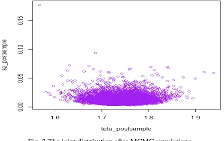
This procedure involves the simulation of 10000 pairs representing independent samples from the joint posterior distribution p(θ,σ2 |y1,y2,...,yn) . Moreover, the simulated values
{
θ(1),...,θ(S)}
represent independent samples from the marginal distributionp(θ| y1,y2,...,yn).
Fig. 2 The joint distribution after MCMC simulations
Fig. 3 The marginal distribution of 1/ σ2
after simulations.
Fig. 4 The marginal distribution of θ after simulations.
A 95% confidence interval for the parameter θ is
(1.72, 1.81).
F. Improper Prior
The problem involved is how Bayesian analysis can be used without prior information from the prior distribution. Many authors, from Lindley in 1973 ([6]) and then Kass in 1996([7]), were doubtful in using the improper priors that are not
probability distributions, instead of prior
distributions. As we refer to the parameters k0 and
ν0 as the prior sample size, it seems as small as
these parameters are then the estimation will be
more objective. This naturally induces to the thought of what happens to the posterior
distribution when k0 and ν0 are reduced
considerably.
The formulas for are:
n k
y n k
n
+ + =
0 0 0µ
µ
− + + − + +
= 2
0 0
0 2 2
0 0 0
2
) ( )
1 ( 1
µ σ
υ υ
σ y
n k
n k s n n
n
When k0,υ0 →0, then we have:
y
n →
µ
∑
−= −
→ 2 2
2 1 1 (y y)
n s n n
i n
σ
These results bring to the following posterior:
{
1/ | y1,y2,...,yn}
2σ ~ 1 ( ) )
2 , 2
(
∑
y −y 2n n n
gama i
{
2}
2 1, ,..., ,
| σ
θ y y yn ~ ( , 2/ )
n y
N σ .
Marking ~p(θ,σ2)=1/σ2 and considering that
) , ( ~ ) , | ( ) | ,
(θ σ2 y p y θ σ2 pθ σ2
p ∝ × , we get the
same conditional distribution for θ but a gamma
distribution for 1/σ2 ([11]). From the integration of the joint distribution from σ2 it comes the result:
1) -S(n ~ ,...y y , y |
/ n 1 2 n
s y
−
θ
, which means that after the sample is made we have that the unknown parameter is given by a student distribution with n-1 degree of freedom. Meanwhile the conditional distribution θ |θ
/ n s Y −
is also with student distribution of n-1 degree of freedom. This means that before the sample is made, the difference of Y from the population mean θ is given by a student distribution of n-1 degree of freedom. The difference lies in the fact that before sampling the two parameters Y and θ are unknown, but after the sample is made then Y = y is known and it provides information about the unknown parameter
θ.
distribution with n-1 degree of freedom, so we are not in the case of proper Bayesian analysis. In the limit, theoretical results according to Stein ([2]) show that from a decision – making point of view, any suitable point estimator is a Bayesian estimator or it is the limit of a sequence of Bayesian estimators and each estimator is suitable ([3]).
IV. BIAS AND MEAN SQUARE ERROR OF THE
ESTIMATORS
A point estimator of an unknown parameter θ is a function that reflects the data in a single parameter of the parameter space Θ. In the case where the sample is made from a normal distribution and we have the conjugate prior distribution previously considered, the posterior estimation of the mean θ is:
0 0 0 0 0 2 1 2 1 ) 1 ( ) ,..., , | ( ) ,..., , ( ˆ µ µ θ θ w y w n k k y n k n y y y E y y
y n n
− + = + + + = = b
The elements of the sample for an estimator
θ
ˆb refer to its behaviour hypothetically based on repeated surveys or evidence. Let’s compare the properties with the mean sampley y y
y , ,..., n)=
( ˆ
2 1 e
θ
when the exact value of the population mean θ0 is known:• E(
θ
ˆe |θ
=θ
0)=θ
0, soθ
ˆe is an unbiased estimator of θ0.• E(
θ
ˆb|θ
=θ
0)=wθ
0+(1−w)µ
0, if µ ≠0 θ0, thenθ
ˆb is biased.The bias shows how close is the centre of the sample distribution for a point estimator with the correct value of the parameter. Generally, an unbiased estimator is desired, however the bias does not indicate how far it is an estimator from the correct value. Consider y1an unbiased estimator of
the population mean, this estimator is further from
θ0 than it is y . To assess the proximity of an
estimator with the correct value θ0, we use the mean
square error (MSE) and if m=E(
θ
ˆ|θ
0) then MSEis:
[
]
[
]
[
] [
]
[
0]
2 0 0 0 0 2 0 2 0 0 2 0 0 | ) ( | ) )( ˆ ( 2 | ) ˆ ( | ) ˆ ( | ) ˆ ( ) | ˆ ( θ θ θ θ θ θ θ θ θ θ θ θ θ θ θ − + − − + − = = − + − = = − = m E m m E m E m m E E MSE
Whilem= E(
θ
ˆ|θ
0), we have E(θ
ˆ−m|θ
0)=0 therefore the second term is zero, that is:) | ˆ ( ) | ˆ ( ) | ˆ ( 0 2 0
0
θ
θ
θ
θ
θ
θ
D biasGMK = +
This means that before the data is collected, the expected distance of an estimator from the correct
value depends on the proximity of θ0 with the
distribution centre and by the variance of
θ
ˆ .Referring to the comparison of the two estimator
b
ˆ
θ
withθ
ˆe, bias(θ
ˆe |θ
0)=0 butθ
ˆbhas the smallestvariability:
n
D e
2 2 0, )
| ˆ (
θ
θ
=θ
σ
=σ
n n w D b 2 2 2 2 0, ) |ˆ
(θ θ =θ σ = ×σ <σ
The mean square errors for the two estimators are:
[
]
n D
E
MSE e e e
2
0 0
2 0
0) (ˆ ) | (ˆ | )
| ˆ (
θ
θ
=θ
−θ
θ
=θ
θ
=σ
[
]
{
}
[
]
2 0 0 2 2 2 0 2 0 0 0 0 2 0 0 ) ( ) 1 ( | ) )( 1 ( ) ( | ) ˆ ( ) | ˆ ( θ µ σ θ θ µ θ θ θ θ θ θ − − + × = = − − + − = − = w n w w y w E EMSE b b
It is true thatMSE(
θ
ˆb |θ
0)<MSE(θ
ˆe |θ
0) when + = − + < − 0 2 2 2 0 0 2 1 1 1 ) ( k n w w n σ σ θ µ .
If there are data on the population from which is made the sample, it is easy to find the values µ0 and
k0 for which the inequality is true. In this case is
built a Bayesian estimator with a square mean distance smaller than sample mean.
If we consider µ0 =100and σ02=225, then:
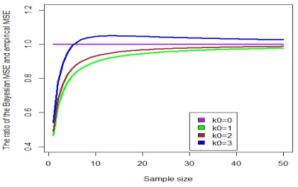
144 ) 1 ( 169 ) 112 | ˆ ( 169 ) 112 | ˆ ( ) | ˆ ( 2 2 0 2 0 0 w n w MSE n n D MSE b e e − + = = = = = = θ θ σ θ θ θ θ
Fig. 5 Bayesian Estimator versus Empirical Estimator MSE
Fig. 5 shows that the MSE for the Bayesian estimator is smaller than the sample mean when k0
=1, 2 and especially when the sample size is small. When k0 =3, the MSE is greater for the Bayesian
estimator but when the size n increases than it is seen that the bias goes to 0.
The Fig. 6 shows the graphs for different values of k0 when n=10 (small sample size) and for the
sample mean.
Fig. 6 The graphs of the distributions for the sample mean and the three Bayesian estimators (yellow, blue, green and magenta respectively).
This graph reinforces the fact that when k0 =1 the
Bayesian estimator’s graph (the blue curve) is closer the real population mean θ0=112 (intersected blue line) and its variance is small. This means that this estimator is closer to the true value of the parameter than the sample mean that is the empirical estimator.
CONCLUSIONS
The normal distribution is very important not only for its wide usage in different models, but even for the fact that the sample mean converges to a normal distribution by the Central Limit Theorem.
This probability distribution belongs to the family of exponential distributions where the mean and the empirical variance of the sample are sufficient statistics for its parameters.
The main benefit from the Bayesian inferential analysis is that it allows for small samples to make a better estimation usually starting from prior information. In this way, the normal distribution is determined by the estimators of its parameters and it can be further used in finding various probabilities we are interested in for different applications.
The main difference between Frequentist and Bayesian schemes is in the different ways of defining the probability. The Frequentist statistics (the classic statistics) treats the probability of events and does not quantify the inaccuracy of the true values of parameters. Instead, Bayesian statistics defines the probability distribution over possible values of a parameter that can be useful in different fields of interest.
REFERENCES
[1] Sir Harold Jeffreys, Theory of Probability, first published in 1939,Oxford Classic Texts in the Physical Sciences, 2000.
[2] Charles Stein, A Necessary and Sufficient Condition for Admissibility, The Annals of Mathematical Statistics, Volume 26, number 3, 1955. [3] James Berger, A Robust Generalised Bayes Estimator and Confidence
Region for a Multivariate Normal Mean, The Annals of Statistics, Volume 8, No4, July 1980, p 716-761.
[4] Bradley P. Carlin, Thomas A. Louis, Bayesian Methods for Data Analysis (Third ed.). Chapman & Hall/ CRC,
Press ISBN9781584886983, pp27–41, 2008.
[5] Christopher M. Bishop, Pattern Recognition and Machine Learning. Springer. pp. 21–24. ISBN978-0-387-31073-2, 2006
[6] Dennis.V. Lindley, O. Barndorff-Nielsen, Gustav Elfving, Erik Harsaae, Daniel Thorburn, Anders Hald and Emil Spjötvoll,The Bayesian Approach. Scandinavian Journal of Statistic, vol 5, no. 1, pp 1-26, 1978.
[7] Robert E. Kass, Larry Wasserman, The selection of Prios distribution by formal rules, Journal of American Statistical Association, Vol 1, No 435, pp 1343-1370, September 1996.
[8] Christian P. Robert and George Casella, Monte Carlo Statistical Methods.Springer-Verlag, New York, second edition, 2004. [9] Christian P. Robert and George Casella, Introducing Monte Carlo Methods with R.Use R! Springer-Verlag, New York, 2009. [10] Christian P. Robert, The Bayesian Choice. Springer-Verlag, New
York,paperback edition, 2007.
[11] Donald B Rubin, Andrew Gelman, John B. Carlin, Hal
Stern, Bayesian Data Analysis (2nd ed.). Boca Raton: Chapman & Hall/CRC. ISBN1-58488-388-X. MR2027492,2003
0.00 0.05 0.10
100 110 120
x
y