Multi Objective Solid Transportation Problem with Interval Cost in Source and Demand Parameters

Multi_Objective Solid Transportation Problem

with Interval Cost in Source and Demand

Parameters

A.Nagarajan, K.Jeyaraman,S.krishna Prabha

Professor, Department of Mathematics, PSNA College of Eng. and Tech., Dindigul- 624 622., Tamil Nadu, India.

Dean, Science and Humanities, PSNA College of Eng. and Tech., Dindigul- 624 622., Tamil Nadu, India

Associate Professor, Department of Mathematics, PSNA College of Eng. and Tech., Dindigul- 624 622., Tamil Nadu, India.

Abstract : In this paper, a solution procedure has been given for the Multi-Objective Interval Solid Transportation Problem under stochastic environment where the cost coefficients of the objective functions have been taken as random variables whereas the source availability, destination demand and conveyance capacities have been taken as stochastic intervals by the decision makers. The problem has been transformed into a classical multi-objective transportation problem where the multiple objective functions are minimized by using fuzzy programming approach. Numerical examples are provided to illustrate the approach.

Keywords: Solid transportation problem; Multi-objective interval solid transportation problem; Stochastic programming; Fuzzy programming

1. Introduction

As a generalization of traditional TP, the Solid Transportation Problem (STP) was stated by Shell [1] in 1955, which, he considered the three item properties in the constraint set instead of two items namely source and destination. He also suggested the situations where the STP would arise, and four cases of STP were discussed according to the data given on the item properties and developed its solution procedure. Basu et al. [2] developed an algorithm for finding the optimum solution for the solid fixed charge linear transportation problem. Although STP was forgotten for long time, because of existing advanced solution methodologies, recently it is receiving the attention of many researchers of this field. Models and algorithms have been developed by many authors [3-9].

In literature, it was found that various effective algorithms were developed for solving transportation problems with the assumption that the coefficients of the objective function, source availability, destination demand and conveyance capacities are specified in a crisp manner. However, these conditions may not be satisfied always. Since in the present situation, the unit transportation costs are rarely constant. To deal the problems with ambiguous coefficients in mathematical programming, inexact and interval programming techniques have been developed by many authors [10- 13].

The STP in uncertain environment becomes important branch of optimization and a lot of models

and algorithms have been presented for different problems by different authors [14, 15, 16, 17]. A.Nagarajan and K.Jeyaraman developed many models and methods for solving multi_ objective interval solid Transportation problems in stochastic environment[20,26,27,28,29,30],solution procedures for solid fixed cost bi-criterion indefinite quadratic transportation problem under stochastic environment [20]. S.K.Das et al. [21], developed the theory and methodology for multi-objective transportation problem with interval cost, source and destination parameters. Expected value of fuzzy variable and fuzzy expected value models presented by Baoding Liu and Yian-Kui Liu [22].

This paper is organized as follows. In Section 2, the basic idea of MOISTP has been given. In Section 3, definitions of interval arithmetic and related definitions have been given. The formulation of crisp objective function and crisp constraint have been given in the section-4 and section-5 respectively. Expected value of MOISTP is given in Section-6. Fuzzy programming approach for the solution of MOISTP is given in Section-7. The numerical example is given in section 8 along with the solution to illustrate the approach.

2.Multi-objective Interval Solid

TransportationProblem (MOISTP)

The MOISTP is a generalization of the multi-objective solid transportation problem in which input data are expressed as stochastic variables as well as stochastic intervals instead of point values. These types of problems arise only when uncertainty occurs in data. The decision makers consider it as more convenient to express it as intervals which can be stated as follows.

Problem-I :

Minimize

Zp =





m

i 1





n

j 1





l

k 1

[c_Lijkp , c_Rijkp ]xijk ,

p = 1, 2, 3,..., P (1) subject to





n

j 1





l

k 1

xijk = [aLi, aRi] ,

i = 1, 2, 3,…, m. (2)





m

i 1





l

k 1

xijk = [bLj, bRj] ,

j =1, 2, 3, ..., n. (3)





m

i 1





n

j 1

xijk = [eLk, eRk ],

k = 1, 2, 3, ... ,l. (4)

with





m

i 1

a_Li≥





n

j 1

b_Lj,





m

i 1

a_Ri≥





n

j 1

b_Rj,





l

k 1

e_Lk ≥





n

j 1

b_Lj,





l

k 1

e_Rk ≥





n

j 1

b_Rj

(non-balanced condition). (5)

Where [c_Lijkp , c_Rijkp ] for p = 1, 2, 3,..., P are intervals

representing the uncertain cost for the transportation problem; it can represent delivery time, quantity of goods delivered, under used capacity, etc. The source

parameter lies between left limit a_Li and right limit a

Ri, similarly, destination parameter lies between left

limit b_Lj and right limit b_Rj and conveyance

parameter lies between left limit e_Lk and right limit e

Rk.

Definition 2.1 [18, 19]

Let





(., /, +, - ) be a binary operation on the set of real numbers. If A and B are closed intervals, then

A



B = { a



b: a



A, b



B } (6) defines a binary operation on the set of closed

intervals. In the case of division, it is assumed that 0



B. The interval operations used in this research paper are as given below.

A + B = [a_L, a_R] + [b_L, b_R ]

=[a_L+b_L,a_R+b_R], (7)

A + B =



a_C, a_W



+



b_C, b_W



=



a_C+b_C, a_W+b_W



, (8) kA = k[a_L, a_R]

= [ka_L, ka_R] for k ≥ 0, (9)

kA = k[a_L, a_R]

= k[a_R, ka_L] for k < 0, (10)

KA = k



a_C,a_W



=



ka_C,

k

a_W



, (11) where ‘k’ is real number.

3. Order relation between Intervals

The order relations which represent the decision makers’ preference between interval costs are defined for the minimization problems. Let the uncertain costs from two alternatives be represented by intervals ‘A’ and ‘B’ respectively. It is assumed that the cost of each alternative is known only to lie in the corresponding interval.

Definition 3.1 The order relation ≤_LR between A

= [a_L, a_R] and B =[b_L, b_R ] is defined as

A ≤_LRB iff a _L ≤ b_L and a_R ≤ b_R, A <_LR B

iff A ≤_LRB and A



B.(12)

This order relation ≤_LR represents the decision makers’ preference for the alternative with lower

Definition 3.2 The order relation ≤_CW between A =



a_C, a_W



and

B =



b_C, b_W



is defined as

A ≤_CWB iff a_C≤ b_C and a_W ≤ b_W A<_CW B iff

A ≤CWB and A



B.(13)

This order relation ≤_CW represents the decision makers’ preference for the alternative with lower expected cost and less uncertainty, i.e., if A ≤_CWB, then A is preferred to B.

4. Formulation of the crisp objective function

In this section, the formulation of original interval objective function has been made as a crisp one.

Definition 4.1 x0



S is an optimal solution of the problem-I iff there is no other solution x



S which satisfies Z(x) <_LRZ(x 0)or Z(x) <_CWZ(x 0).

Theorem 4.1 It can be proved that A ≤_RC B iff A

≤_LR B or A ≤_CW B,A <_RC B iff A <_LRB or A

<_CW B, (14)

where the order relation ≤_RC is defined as

A ≤_RC B iff a_R ≤ b_Rand a_C≤ b_C, A <_RCB

iff A ≤_RC B and A



B.

Using the theorem 4.1, Definition 4.1 is simplified as follows.

Definition 4.2 x0



S is an optimal solution of the Problem-I iff there is no other solution x



S which satisfies

Z(x) <_RC Z(x 0).The right limit

ZP_R( x) of the interval objective function in problem-I is derived from the equations (8) and (11) as

Z_Rp(x) =





m

i 1





n

j 1





l

k 1

c_Cijkp xijk +





m

i 1





n

j 1





l

k 1

c_Wijkp

ijk

x

(15)

where c_Cijkp is the centre and c_Wijkp is the half width

of the coefficient of xijk in

p

.

In the case when xijk ≥ 0, i = 1, 2, 3,…, m, j = 1, 2, 3, ..., n, k = 1, 2, 3, …, l,

ZP_R( x) is modified as:

Z _Rp (x) =





m

i 1





n

j 1





l

k 1

c_Cijkp xijk +





m

i 1





n

j 1





l

k 1

c_Wijkp xijk. (16) The

centre of the objective function Z_Cp(x) for the Problem–I can be defined as

Z_Cp(x) =





m

i 1





n

j 1





l

k 1

c_Cijkp xijk. (17)

The solution set of the Problem-I defined by Definition 4.2 is also obtained as the Pareto optimal solution of the two multi-objective problem as:

Minimize { Z_Rp, Z_Cp}, p = 1, 2, 3,…,P,

subject to the constraints (2) – (5) respectively

where Zp_R and Z_Cp are as stated as in equations (16)

and (17).

5. Formulation of the crisp constraint

By using the theory of interval arithmetic [18,19], the Problem-I is converted into its equivalent form as follows .

Problem -II:

Minimize

Zp =





m

i 1





n

j 1





l

k 1

[c_Lijkp , c_Rijkp ]xijk ,

p= 1, 2, 3,..., P (18) subject to





n

j 1





l

k 1

xijk



aLi,

i = 1, 2, 3,…,m. (19)





n

j 1





l

k 1

xijk



aRi,

i = 1, 2, 3,…,m. (20)





m

i 1





l

k 1

xijk



bLj,

j = 1, 2, 3, ..., n. (21)





m

i 1





l

k 1

xijk



bRj,

j = 1, 2, 3, ..., n. (22)





m

i 1





n

j 1

k = 1,2,3,…, l. (23)





m

i 1





n

j 1

xijk



eRk,

k=1,2,3,…,l. (24) xijk≥0 ,for all i, j, k.





m

i 1

a_Li≥





n

j 1

b_Lj





m

i 1

a_Ri≥





n

j 1

b_Rj,

x

ijk

*

e_Lk ≥





n

j 1

b_Lj,





l

k 1

e_Rk≥





n

j 1

b_Rj

(non balanced condition). (25)

6. Expected value of stochastic variable

In this section, the expected value of a stochastic variable is defined.

Definition 6.1 Let ‘



’ be a random variable whose expected value is defined by

E[



] =





0

Pr {



≥ r }dr -



 

0

Pr{



≤ r }dr

provided that at least one of the two integrals is finite where r





[14].

Let ‘



’ and ‘



’ be random variables with finite expected values. For any values of ‘a’ and’ b’ it has been proved that

E[a



+ b



] = aE[



] + bE[



]. i.e, the

expected value operator has the linearity property.

Theorem 6.1 Let ‘



’ be a random variable whose

probability density function ‘



’ exists. If the

Lebesgue integral





 

x



(x)dx is finite, then it is

arrived as E[



] =





 

x



(x)dx.

6.1 Expected value model for MOISTP

The expected value model (EVM) which optimizes some expected objective function subjected to some expected constraints, for example ,minimizing the expected time, minimizing expected cost, maximizing expected profit etc. Normally if we want to find a decision with maximum expected return subjected to some expected constraints then we have the following EVM,

max E [f(xijk ,



)] subject to

E [gj(xijk ,



)] ≤ 0 , j = 1,2,3,…, p

Where . xijk is a desicion vector ,



is a stochastic

vector, f(xijk ,



) is the return function, gj(xijk,



) are stochastic constrained functions for j = 1,2,3,…, q.

Definition 6.2

A solution xijk is feasible if and only if gl(xijk ,



) ≤ 0

, j = 1,2,3,…, p. A fesiable solution is an optimal

solution to EVM if E [f(𝑥𝑖𝑗𝑘∗ ,



)] ≥ E [f(xijk ,



)]

for any feasible solution xijk.

In n multiple objective problems we employ the following expected value multiobjective programming (EVMOP).

max E [f1(xijk ,



),] , E [f2(xijk ,



),]

E [f3(xijk ,



),] ….E [ft(xijk ,



),]

subject to

E [gl(xijk ,



)] ≤ 0 , l = 1,2,3,…, q

where fr(x ,



) are return functions for

r = 1, 2,3,….t

Definition 6.3

A feasible solution 𝑥_𝑖𝑗𝑘∗ is said to be pareto optimal solution to EVOMP if there is no feasible solution xijk such that

E [fi(xijk ,



),] ≥ E [f1(𝑥𝑖𝑗𝑘∗ ,



),]

r = 1,2,3,….t and

E [fl(xijk ,



),] > E [fi(𝑥𝑖𝑗𝑘∗ ,



),]

for atleast one index l

The expected value model EVM for the problem II defined in section 5 takes the form

Problem - III: Minimize

Zp=





m

i 1





n

j 1





l

k 1

[c_Lijkp , c_Rijkp ]xijk

p = 1, 2, 3,…,P, subject to:

E[





n

j 1





l

k 1

xijk - aLi] ≥0, i =1,2,3,…, m.

E[





n

j 1





l

k 1

xijk - aRi ] ≤ 0, i =1,2,3,…, m.

E[





m

i 1





l

k 1

xijk – bLj] ≥ 0, j =1,2,3, ..., n. E[





m





l

k 1

xijk – bRj] ≤ 0, j =1,2,3,..., n. E[





m

i 1





n

j 1

xijk –

e_Lk] ≥ 0, k=1,2,3,…, l. E[





m

i 1





n

j 1

xijk – eRk] ≤ 0 , k

=1,2,3, …, l. where xijk ≥ 0 , for any i, j, k.

The problems proposed in the previous sections are constructed under stochastic environment. In order to find the suitable solution for the problems, the expected value, critical value or credibility measure must be calculated. If the stochastic parameters are complex, the computing objective values subject to the constraints becomes a time consuming one. Due to this, it is better to convert the models into their crisp equivalents by using the appropriate probability levels defined by the decision makers.

By using the linearity of expected value operator of random variable, the Problem–III is equivalent to

:

Problem IV: Minimize

Zp =





m

i 1





n

j 1





l

k 1

[c_Lijkp , c_Rijkp ]xijk

p = 1, 2, 3,…,P, subject to:





n

j 1





l

k 1

xijk



E[aLi], i = 1,23,…, m.





n

j 1





l

k 1

xijk



E[aRi ], i =1,2,3,…, m.





m

i 1





l

k 1

xijk



E[bLj], j =1,2, 3, ..., n.





m

i 1





l

k 1

xijk



E[bRj] j =1,2, 3, ..., n.





m

i 1





n

j 1

xijk



E [eLk] ,k =1,2,3,…, l.





m

i 1





n

j 1

xijk



E[eRk] , k =1,2,3, …, l.

where xijk ≥ 0 , for any i, j, k.

7.FuzzyProgramming approach for MOISTP The MOISTP can be considered as a vector minimum problem. The first step to solve the problem is to assign, for each objective, two values U

p

and Lpas upper and lower bounds, respectively,

for the p-th objective, where Upis the highest acceptable level for achievement for the p-th

objective, Lpis the aspired level of achievement for

the p-th objective and dp= Up- Lpis the degradation allowance for the p-th objective. Once the aspiration levels and degradation allowance for each objective have been specified, we have formed the fuzzy model and then convert the fuzzy model into a crisp model. The steps of the fuzzy programming approach may be summarized as follows.

Algorithm:

Step 1. Solve the multi-objective interval solid transportation problem using one objective at a time(ignoring all others) subject to the given set of constraints by using any one of the suitable

evolutionary technique. Let X1*= {x1_ijk }, X2*= {x

2

ijk}, X

* 3

= {x3_ijk},…, XP* = {x_ijkp } be the optimum solutions for P different single objective interval solid transportation problems.

Step 2. From the results of step1, the values of all the objective functions will be calculated at all these ‘P’ optimal points. Then a payoff matrix is formed. The diagonal of the matrix constitutes individual optimum

minimum values for the P objectives. The ‘XP*’’s are the individual optimal solutions and each of these are used to determine the values of other individual objectives, thus the payoff matrix is developed as follows:

X1* X2* … XP* Z1 Z1( X1*) Z1(X2*) ... Z1 ( XP*) Z2 Z2( X1*) Z2( X2*) … Z2( XP*) Z3 Z3( X1*) Z3 ( X2*) … Z3( XP*)

Zp Zp( X1*) Zp( X2*) … Zp( XP*)

We find the upper and lower bound for each

objective from the payoff matrix. Here Lp= Zp(X

*

P

) and Up= max{

Zp( X1*), Zp( X2*), …, Zp( XP*)}.

Step 3. The initial fuzzy model is given by the aspiration level with each objective as follows: Find xijk i =1,2,3,…,m, j =1,2,3,...,n and k=1,2,3,...,l,

so as to satisfy Zp



Lp where p = 1, 2, 3,…,P, and the given constraints and non-negativity conditions.

Step 4. For the multi-objective interval solid

1 if Zp



Lp



p(Zp)=

















p p

p p

L

U

Z

U

IfLp<Zp<Up

0 if Zp



Up,

Where Up



Lpforall p. If Up= Lp for all p then

p



(Zp) = 1 for all p.

Step 5. Formulate a fuzzy linear programming problem. By using max-min operator, the equivalent fuzzy linear programming problem for the multi-objective interval solid transportation problem is formulated as follows:

For right limit of the objective function ZP_R(x), the fuzzy linear programming problem is obtained as Maximize



subject to





m

i 1





n

j 1





l

k 1

{c_Cijkp +c_Wijkp }xijk +



(U

p

- Lp)



Up, p = 1, 2, 3,...,P, with the given constraints and





0, where



= min {



p(Zp)}.

For the centre of the objective function Z_Cp(x), the

fuzzy linear programming problem is obtained as

Maximize



subject to





m

i 1





n

j 1





l

k 1

c_Cijkp xijk+



(U

p

- Lp )



Up, p =

1, 2, 3,...,P, with the given constraints and





0, where



= min {



p(Zp)}.

Find out an optimal solution of the foregoing problem by using any existing method. Substituting this optimal value in each objective we get an optimal compromise interval of each objective.

8. Numerical Example:

When the objective functions’ coefficients

c_ijkp are in the of random variables but the source,

destination and conveyance parameters a_i, b_jand e

kare in the of stochastic intervals, the multi-objective

interval solid transportation problem can be stated as follows:

MinimizeZp =





m

i 1





n

j 1





l

k 1

c_ijkp xijk ,

p = 1, 2, 3,..., P (33) subject to





n

j 1





l

k 1

xijk = [aLi, aRi], (34)





m

i 1





l

k 1

xijk = [bLj, bRj], (35)





m

i 1





n

j 1

xijk = [eLk, eRk ], (36)

with





m

i 1

a_Li≥





n

j 1

b_Lj,





m

i 1

a_Ri≥





n

j 1

b_Rj,





l

k 1

e_Lk.

where xijk ≥ 0 , for any i = 1, 2, 3, …, m, j = 1, 2, 3, …,n and k = 1, 2, 3, …,l.

Using the expectation of random variables the above problem is equivalent to

Minimize Zp =





m

i 1





n

j 1





l

k 1

c_ijkp xijk ,

p = 1, 2, 3,..., P subject to





n

j 1





l

k 1

xijk



E[aLi],





n

j 1





l

k 1

xijk



E[aRi ],





m

i 1





l

k 1

xijk



E[bLj],





m

i 1





l

k 1

xijk



E[bRj],





m

i 1





n

j 1

xijk



E [eLk] ,





m

i 1





n

j 1

xijk



E[eRk] ,

where xijk ≥ 0 , for any i = 1, 2, 3, …, m, j = 1, 2, 3, …,n and k = 1, 2, 3, …,l. The solution procedure has been illustrated in the following numerical example.

Example

MinimizeZ1 =





3

1

i





3

1

j





2

1

k

MinimizeZ2 =



 3 1 i



 3 1

j





2

1

k

c2_ijkxijk

subject to





3

1

j





2

1

k

x1jk = [N(32,5), N(90, 7)],





3

1

j





2

1

k

x2jk = [N(40, 5), N(95,7)],





3

1

j





2

1

k

x3jk = [N(36,7), N(98, 4)],





3

1

i





2

1

k

xi1k = [EXP 20), exp(35)],





3

1

i





2

1

k

xi2k = [EXP 15), exp(43)],





3

1

i





2

1

k

xi3k = [EXP p(20), exp(40)],





3

1

i





3

1

j

xij1 = [U(25, 65), U(36, 80)],





3

1

i





3

1

j

xij2 = [U(23,50), U(60, 80)].

where xijk ≥ 0 , for i , j = 1, 2, 3, k = 1, 2.

Using the expectation of random variables the equivalent deterministic MOISTP is written as:

MinimizeZ1 =



 3 1 i



 3 1

j





2

1

k

c1_ijk xijk

MinimizeZ2 =



 3 1 i



 3 1

j





2

1

k

c2_ijkxijk

subject to





3

1

j





2

1

k

x1jk



32,





3

1

j





2

1

k

x1jk



90,





3

1

j





2

1

k

x2jk



40,





3

1

j





2

1

k

x2jk



95,





3

1

j





2

1

k

x3jk



36,





3

1

j





2

1

k

x3jk



98,





3

1

i





2

1

k

xi1k



20,





3

1

i





2

1

k

xi1k



35,





3

1

i





2

1

k

xi2k



15,





3

1

i





2

1

k

xi2k



43,





3

1

i





2

1

k

xi3k



20,





3

1

i





2

1

k

xi3k



40,





3

1

i





3

1

j

xij1



45,





3

1

i





3

1

j

xij1



58,





3

1

i





3

1

j

xij2



36.5,





3

1

i





3

1

j

xij2



70.

where xijk ≥ 0 , for i , j = 1, 2, 3, k = 1, 2,

c1_ijk (Table-3) and c_ijk2 (Table-4) are cost matrices for the criterians 1 and 2 respectively.

Using fuzzy approach, the pareto optimal

solution of the problem is obtained as x₁₂₁= 5.2854, x₁₃₁= 26.7146,

x₂₁₂= 29.3573, x₂₂₁= 7.3573, x₂₃₂=3.2854, x₃₁₁= 5.6427, x₃₂₂= 30.3573,



=0.7784 and other x_ijk are zeros. Z1 = 870.71 and Z2= 778.0719.

,

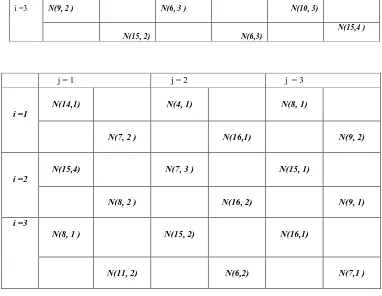
Table–1. Interval cost matrix consisting of 3 sources, 3 destinations and 2 conveyances for second criterion.

j = 1 j = 2 j = 3

i =1

N(15,1) N(13, 4)

N(7, 1)

N(12, 1) N(7, 2 ) N(9, 4 )

i =2

N(14, 3) N(12, 3) N(7, 2 )

Table – 2. c2_ijktransportation cost for second criterion.

9. CONCLUSION

This paper proposes a solution procedure for multi-objective interval solid transportation problem under stochastic environment using fuzzy programming approach. All source availability, destination demand and conveyance capacities have been taken as stochastic intervals for each criterion. Expectation of a random variable has been used to transform the problem into a classical multi-objective transportation problem where the multi-objectives which are the right limit and centre of the interval objective functions are minimized. The main advantage of fuzzy programming is that, for a MOISTP with ‘p’ objective functions, this approach leads to p non-dominated solutions and one optimal compromise solution, whereas other algorithms leads to more than p non-dominated and dominated solutions from which the decision maker can choose a compromise solution.

References:

[1] E.Shell, Distribution of a product by several properties,

Directorate of Management Analysis, Proc. 2nd _{Symp. on}

Linear programming, Vol. 2, 1955, pp. 615-642, DCS/Comptroller H.Q. U.S.A.F., Washington, DC.

[2] Basu, M., Pal, B.B., and Kundu, A., An algorithm for optimum solution of solid fixed-charge transportation

problem , Optimization31 (1994) 283-291.

[3] A.K.Bit, M.P.Biswal, S.S.Alam, Fuzzy programming approach to multi-objective solid transportation problem, Fuzzy Sets Systems. 57(1993) 183-194. [4] F.Jimenez, J.L.Verdegay, Uncertain solid transportation

problems, Fuzzy sets systems.100 (1998) 45-57.

[5] Lixing Yang and Linzhong Liu, Fuzzy fixed charge solid

transportation problem and algorithm , Applied soft

computing , 7(2007) 879-889.

[6] F.Jimenez, J.L.Verdegay, Solving fuzzy solid transportation problems by an evolutionary algorithm based

parametric approach, European Journal of Operations

Research, 117(1999) 485-510.

[7] Y.Li, K.Ida, M.Gen, R.Kobuchi, Neural network approach for multicriteria solid transportation problem,

Comput. Ind. Eng.33(1997) 465-468.

[8] Y.Li, K.Ida, M.Gen, Improved genetic algorithm for solving multiobjective solid transportation problem with fuzzy numbers, Comput. Ind. Eng. 33(1997) 589-592.

[9] M.Gen, K.Ida, Y.Li, E.Kubota, Solving bicriteria solid transportation problem with fuzzy numbers by a genetic

algorithm, Comput. Ind. Eng. 29(1995) 537-541.

[10] M.Inguichi, Y.Kume, Goal programming problem with

interval coefficient and target intervals, European Journal

of Operations Research52 (1991) 345-360.

[11] R.E.Stuer, Algorithm for linear programming problems with interval objective function coefficient, Mathematics of Operations Research6 (1981) 333-348.

[12] S.Tong, Interval number and fuzzy

i =3 N(9, 2 ) N(6, 3 ) N(10, 3)

N(15, 2) N(6,3)

N(15,4 )

j = 1 j = 2 j = 3

i =1

N(14,1) N(4, 1) N(8, 1)

N(7, 2 ) N(16,1) N(9, 2)

i =2

N(15,4) N(7, 3 ) N(15, 1)

N(8, 2 ) N(16, 2) N(9, 1)

i =3

N(8, 1 ) N(15, 2) N(16,1)

number linear programming, Fuzzy Sets and Systems66 (1994) 301-306.

[13] H.Ishibuchi, H.Tanaka, multiobjective programming in optimization of the interval objective function, European Journal of Operations Research 48 (1990) 219-225. [14] B.Liu, Theory and Practice of Uncertain Programming,

Physica-Verlag, New York, 2002.

[15] B.Liu , Depenedent chance programming with fuzzy decisions, IEEE Transactions on Fuzzy Systems, 7(3) (1999)354-360.

[16] Lixing Yang and Linzhong Liu, Fuzzy fixed charge solid transportation problem and algorithm , Applied soft computing , 7(2007) 879-889.

[17] Lixing Yang, Yuan Feng, A bicriteria solid transportation problem with fixed charge under stochastic environment,

Applied Mathematical Modeling31 (2007) 2668-2683. [18] G.Alefeld, J.Herzberger, Introduction to Interval

computations, Academic Press, New York, 1983. [19] R.E.Moore, Method and Applications of Interval Analysis,

SLAM, Philadephia, PA, 1979.

[20] A.Nagarajan, K.Jeyaraman, Mathematical modeling of solid fixed cost bi-criterion indefinite quadratic transportation

problem under stochastic environment, Emerging journal

of engineering science and technology, Volume-02, N-03, March2009 – May 2009, pp.106 – 127.

[21] S.K.Das, A.Goswami and S.S.Alam, Multi-objective transportation problem with intervsl cost, source and

destination parameters, European Journal of Operations

Research117(1999)100-112.

[22] Baoding Liu and Yian-Kui Liu, Expected value of fuzzy

variable and fuzzy expected value models, IEEE

Transactions on Fuzzy Systems,10(4) (AUGUST 2002) 445-450.

[23] L.A.Zadeh, Fuzzy sets, Information and control 8 (1965) 338-353.

[24] J.Zimmerman, Fuzzy programming and Linear programming with several objective functions, Fuzzy Sets and Systems

1(1978) 45-55.

[25] H.Liberling, On finding compromise solutions for

multicriteria problems using the fuzzy min-operator, Fuzzy

Sets and Systems6(1981) 105-118.

[26] A.Nagarajan and K.Jeyaraman, Mathematical modeling of

solid fixed cost bi-criterion indefinite quadratic

transportation problem under stochastic environment,

Emerging journal of engineering science and technology, Volume-02, Issue No-03, March 2009 – May 2009, pp.106 – 127.

[27] A.Nagarajan and K.Jeyaraman, Solution of expected value model for multi-objective interval solid transportation problem under stochastic environment using fuzzy

programming approach, Emerging journal of engineering

science and technology, Volume-04, Issue No-07, September 2009 – November 2009, pp. 53 – 70.

[28] A.Nagarajan and K.Jeyaraman, Chance constrained goal programming models for multi-objective interval solid transportation problem under stochastic environment,

International journal of applied mathematics analysis and applications, Volume-05, Issue No-02, July-December 2010, pp. 229 – 255.

[29] A.Nagarajan and K.Jeyaraman, Solution of chance constrained programming problem for multi-objective interval solid transportation problem under stochastic

environment using fuzzy approach, International journal

computer applications, Volume-10- No .9, November 2010, pp. 19 – 29.

[30] A.Nagarajan and K.Jeyaraman, Theory and Methodology chance constrained programming model for multi-objective interval solid transportation problem under

stochastic environment using fuzzy approach, Proceedngs

of International conference on emerging trends in