Ab s t r a c t.The CRPSM model developed by Hillet al. (1996) was modified, calibrated and tested using cowpea-water use and weather data collected under line source sprinkler system at Ile-Ife, Nigeria. Three sets of data were collected. The first was used to calibrate and modify the model and the other two for testing. Simulated irrigation schedules were then applied using two of the four management options in the model to select the best schedules for the region. The water yield index (WYI) defined as the products of the model predicted relative yield (percent) and the transpiration water ratio (transpiration/water applied) was used to select the best schedule.
The results showed that WYI ranged from 52% for irrigation level one in 1999 to 8% for irrigation level five in 1997, when the model was appliedto actual field data. However, with simulation runs, a six day interval provided a WYI of 66% for irrigation level one in 1999 and a two day interval provided a WYI of 9% for irrigation level five in 1997 using almost the same amount of water. The model, therefore, proved to be useful in estimation of possible irrigation schemes to maximize yields.
K e y w o r d s:cowpea yields, water use index, irrigation scheduling, modelling
INTRODUCTION
Nigeria has two distinct seasons – the rainy season, lasting from mid of March to the end of October, and the dry season, lasting from November to March. In the dry season, there is virtually no rain and irrigation remains the only option for crop production. Cowpea is a major crop produ-ced by irrigation, using mostly the sprinkler system. There is stiff competition for water by the agricultural, domestic and industrial users during the dry season, hence there is the need for farmers to conserve and make judicious use of the availa-ble water. The crop water use efficiency has been shown to depend on irrigation amount and frequency (Adekalu and Okunade, 2006; Fapohunda, 1992). Also the type of
irri-gation system (Yohannes and Tadesse, 1998) and tillage practices (Adekalu and Okunade, 2006; Kayombo et al., 2002) can influence the water use efficiency for a given irri-gation frequency. The irriirri-gation number, amount and uni-formity of water applications are used mainly to determine the efficiency of irrigation scheduling. Excessive doses of infrequently applied water will lead to high percolation losses. The water saved by reducing drainage losses can be used to obtain higher yields by giving additional application to irrigate other farmlands or to store it as an insurance against the more severe periods of drought. While real-time irrigation schedulers can be used to maximize the yield for a specific growing season, they are less useful for planning and management as simulation models.
In this study, the crop yield and water management simulation model (CRPSM) developed by Hillet al. (1996) was modified and calibrated with application to actual field data on cowpea from Nigeria. The field experiment was car-ried out using a line source sprinkler system to generate sets of water use-yield data. The study was done in an attempt to determine some possible irrigation schedules that can opti-mise water use. The CRPSM model was selected because of its simplicity and minimum data requirement, which will make it attractive to developing countries.
MATERIALS AND METHODS
Model description
The crop yield and water management simulation model (CRPSM) developed at Utah State University (Hillet al., 1996) predicts crop phenologic stages and shows the effects of climate, planting date and soil-water crop inter-actions on yield.
Simulating the effects of irrigation scheduling on cowpea yield
K.O. Adekalu
Agricultural Engineering Department, Obafemi Awolowo University, Ile-Ife, Nigeria Received May 16, 2006; accepted September 28, 2006
© 2006 Institute of Agrophysics, Polish Academy of Sciences Corresponding author’s e-mail: [email protected]
w w
The model consists of a main program and twelve subroutines. The model simulates an actual field experiment by computing daily available soil moisture in each layer and daily potential and actual evapotranspiration given the required site, soil, crop, and weather information. If desired, any of the four different irrigation options could be used in the management option in the model; the four irrigation options are:
1. Finding the best day to irrigate with a specified water increment.
2. Irrigating at a specified interval with fixed amount. 3. Irrigating on specified dates with specified amounts
(historical data).
4. Irrigating at a specified depletion with a fixed amount. The model was modified by adding: (1) coefficient to allow for drainage below field capacity in the root zone; (2) runoff equation and (3) coefficient to allow evaporation to depend on the soil water content at the start of soil drying.
Seasonal yield is determined as a function of relative transpiration:
Y Y
T T
T T
T T
T T
m p p p p
=é ë
ê ù
û ú é
ë
ê ù
û ú é
ë
ê ù
û ú é
ë 1
1 1
2
2 2
3
3 3
4
4
l l l
ê ù
û ú é
ë
ê ù
û ú l4 l
5
5 5
T Tp
, (1)
in whichYandYmare actual and potential yields (t ha-1), respectively,TiandTpiare actual and potential transpiration (mm), respectively, andliis growth stage weighing factor for stagei.
Potential evapotranspiration,ETP, is calculated as:
ETp=K ETc r. (2)
Potential transpiration (Tp) is defined as:
Tp=K ETt r, (3)
in whichKc,Kt are crop water use and crop transpiration coefficients, respectively, obtained from a separate lysime-ter experiment, and ETr is reference crop evapotranspi-ration (mm), obtained using the Penman-Monteith equation (FAO, 1998).Ktis a fraction ofKcused to splitETpinto potential transpiration and evaporation based on the leaf area index. Values of crop water use coefficientKc, have earlier been reported by Adeogun and Ahaneku (2002).
Actual transpiration,T, is:
T= Tp when SWS/AVW >FAW, (4)
T= (Tp/FAW) (SWS/AVW) (5)
whenSWS/AVW <FAW,
in whichSWSis existing soil moisture in the root zone (mm),
AVWis available moisture at field capacity (mm); andFAW
is the fraction of available water below which plant stress occurs.
Potential evaporation,Ep, is defined as:
Ep=ETp-Tp. (6)
Actual evaporation,E, is defined as:
E=aEp/N(t-1), (7) a q q= 1/ f1, (8)
in which t is time in days after irrigation, N is a factor depending on soil texture (N= 3.0 and 3.5 for sandy loam and sandy clay loam soils used in this study, respectively), q1is moisture content after irrigation in top 30 cm soil depth
(m3m-3), andqf1is moisture content at field capacity in the
top 30 cm soil depth (m3m-3).
Root depth,RT, is computed in the model as:
RT=BR+RDPTH RTMX( -BR), (9)
where: BR is the initial root depth (mm); RTMX is the maximum root depth (mm); andRDPTHis the ratio of days since emergence to total days from emergence toRTMX.
Deep percolation, DP, and soil moisture content are then determined from the soil water budget equation as:
DPi=(qi-FCi)Zi+B FCi( i-PWP Zi) i,
IFq >i FCi, (10)
otherwise
DPi=Bi(qi-PWP Zi) i, (11)
qi=(qis iZ +DP(i-1))Zi, (12)
where:qiis moisture content of a given soil layer in the root zo-ne (m3m-3), Biis the drainage coefficient for theithlayer in the root zone (the root zone was divided into two distinct layers),FCiis moisture content at field capacity (m3m-3), Ziis the soil depth (mm),PWPiis moisture content at wilting point (m3m-3),qisis the initial moisture content of a given layer (m3m-3),DPiis the deep percolation from a given layer (mm), andDP(i– 1)is the deep percolation from the
preceding layer (mm).
Actual evapotranspiration,ETa, is defined as:
ETa= +E T. (13)
Transpiration water ratio, TWR, defined by actual transpiration/ total water supply, indicates the efficiency of the water consumed by plants relative to the total amount of water made available during the season.
Runoff was calculated as:
R= -P FTr-Sw, (14)
The water yield index,WYI, is defined as:
WYI=PRYxTWR, (15)
where:PRYis the model predicted relative yield (percent of potential yield) andTWRis transpiration water ratio.
Input data required by the model include: site elevation, longitude and latitude, root zone depth, soil layers thickness, initial moisture content, wilting point and field capacity of each layer, weather data for the calculation of reference crop evapotranspiration by Penman-Monteith, Blanney-Criddle, Jensen-Haise, Hargreaves, Thornwaith or pan-evaporation in the model, dates of growth stages and harvest.
Field experiment
The experiment was conducted on a piece of land near the dam at the Teaching and Research Farm of the Obafemi Awolowo University, Ile-Ife, Nigeria. The approximate plot dimension was 30 x 60 m, including border areas and a walking path, 1 m wide, running between adjacent sub plots. The land was ploughed and harrowed after slashing the shrub. Cowpea (Vigna unguiculata, L Walp) variety VITA5 was planted at the recommended spacing of 30 cm on rows, 60 cm apart. Weeds and insect pests were control-led as necessary using standard procedures.
A line source irrigation system developed by Hankset al. (1976), consisting of a single line of sprinklers spaced 6.1 m apart, provided uniform water distribution parallel to the irrigation line and a water gradient perpendicular to the irrigation line. Preliminary tests showed that in the absence of wind the water application pattern was constant in time. The irrigation line was placed on a central guard line and depths of water application to each line on both sides of the irrigation line were measured at each irrigation. The line source created five irrigation levels decreasing from rate 1 to 5. The farthest level from the line, irrigation level 5 (IL5), (either east or west) received very little irrigation (about 100 mm including rainfall) while irrigation level 1 (1L1), just adjacent to the line, received a maximum water supply (average of about 280 mm). The line source irrigation system used impact sprinklers rain bird 30, 4.76 by 2.38 mm – 70° slotted nozzles spaced at 6.1 m along the lateral. Pressure at the inlet averaged 300 kPa and the average discharge per sprinkler was 0.5 l s-1with a wetted area 30 m in diameter. The experiments were conducted on different fields for three years (1995, 1997, and 1999). The 1995 data were used for calibration and those of 1997 and 1999 were used for testing. The soil for 1995 and 1997 is a sandy loam soil classified as an Alfisol while that of 1999 is a sandy clay loam soil classified as Inceptisol (Soil Survey Staff, 1992). Soil water contents were monitored before and after each irrigation using gravimetric and neutron probe for the top 15 cm and neutron probe over a range of 75 cm at an
increment of 15 cm. Soil matric potential values were measured over the same range using tensiometers. Meters were only installed at irrigation levels 1, 3 and 5 in 1995 and 1997, and at irrigation levels 1, 2 and 3 in 1999.
The moisture retention characteristic was measured using standard pressure plates on undisturbed soil cores. The drainage and actual evapotranspiration were estimated from the mass balance of the water content profiles over the wetted depth using the zero-flux plane method (Mcgowan and Williams, 1980). Weather data were obtained from the station at the Farm and used to estimate reference crop evapo-transpiration, according to Penman-Monteith equation (FAO, 1998). Irrigation was scheduled according to estima-ted crop evapotranspiration.
Irrigation/rainfall depths were measured using catch cans placed at right angles to the line source. There were two cans per irrigation level. Rainguages were placed at two rows alongside the catch cans. The readings of the rainguages were used to calibrate the catch cans data. The dates of attainment of the various phenologic stages were observed and recorded. The root depth was monitored at the end of each growth stage and linear interpolation of values was used between the stages. The root monitoring was done by taking soil cores (5 cm in diameter and 5 cm deep) up to 75 cm, two on either side of the first irrigation level, and for each depth; soil samples were combined to give a composite and living root obtained by washing with congo red. At the end of the season, the crops were harvested separately for each row. The pods were removed and weighed. The weight was converted to yield per hectare using the row spacing.
Data from the yield in 1995 were used to determine the growth period weighing factors,l’s, and other parameters in the yield equation. The calibration of the yield equation was done with a pattern search technique (Hillet al., 1972) using field-estimated transpiration by growth stages and the actual yield. The growth session was divided into five stages as follows:
– planting to emergence,
– emergence to beginning of flowering,
– beginning of flowering to beginning of pod fill, – beginning of pod fill to end of flowering and – end of flowering to physiological maturity.
RESULTS AND DISCUSSION Results of calibration and testing
Kt= – 0.17437X1– 0.26124X12+ 0.12870X13+ 0.853623
(P< 0.05), (16)
where X1is ratio of days since emergence to effective cover:
Kt= – 0.14333X2+ 0.20473X22– 0.546451X23+ 0.639725
(P< 0.05), (17)
where X2is period after effective cover (days).
The calibrated yield parameter values werel1= 0.0,l2= 0.4,l3= 1.8,l4= 1.2,l5= 0.6 and a potential yield of 1.8 t
ha-1. The calibrated values for Bi’s were 0.02 and 0.01 for
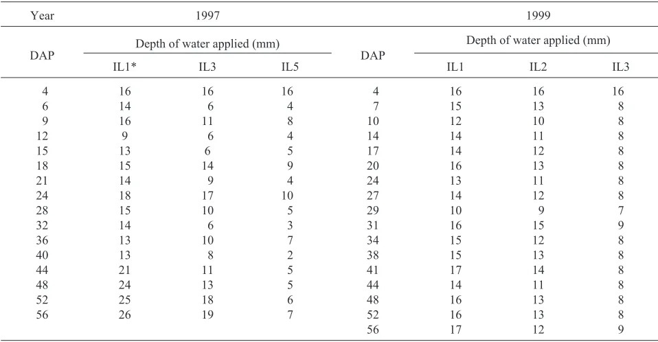
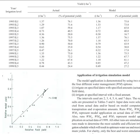
the two soil layers, respectively andSwwas 1 mm.Table 1 shows the depth of water applied for each level whileTable 2 shows the values of predicted yield against measured yield. Figure 2shows the plot of predicted relative yields against measured relative yields for the three years. The 1997 and Fig. 1.Cowpea crop transpiration coefficient curve.
Year 1997 1999
DAP
Depth of water applied (mm)
DAP
Depth of water applied (mm)
IL1* IL3 IL5 IL1 IL2 IL3
4 6 9 12 15 18 21 24 28 32 36 40 44 48 52 56
16 14 16 9 13 15 14 18 15 14 13 13 21 24 25 26
16 6 11 6 6 14 9 17 10 6 10 8 11 13 18 19
16 4 8 4 5 9 4 10 5 3 7 2 5 5 6 7
4 7 10 14 17 20 24 27 29 31 34 38 41 44 48 52 56
16 15 12 14 14 16 13 14 10 16 15 15 17 14 16 16 17
16 13 10 11 12 13 11 12 9 15 12 13 14 11 13 13 12
16 8 8 8 8 8 8 8 7 9 8 8 8 8 8 8 9 *Irrigation level.
1999 data served as independent data set.Table 3shows the comparison between model predicted and actual soil water budget parameters. The table shows that the model gave very good estimates that agreed with field values. The agree-ment was better under the highest irrigation level. These results have increased the confidence in using the model for selecting irrigation schedules and for predicting yields.
Table 4 shows the theoretical values of the water requirement. From the table, it can be noted that the theore-ticalKcis a little higher than the actualKcvalues (Table 3), indicating that the first irrigation levels in both years almost received their optimum water requirements.
Application of irrigation simulation model
The model application is demonstrated by using two of the four different water management (WM) options: (i) irrigate on specified dates with specified amounts (actual field data),
(ii) irrigate at specified interval with a fixed amount.
The intervals used are 2, 3, 4, 5, 6, and 7 days. The re-sults are presented in Tables 5 and 6. Input data were sele-cted from actual data and/or based on model computed transpiration and evaporation amounts. RunsWM1,WM4, WM7 represent model application on actual data of 1997. Also, runs WM1, WM4, and WM7 represent model ap-plication on actual data of 1999. All other runs are simulated runs made to determine the most suitable and efficient irri-gation schedule which will result in optimum water use and maxi-mum yields. For clarity, only the best and worst simulation runs are presented.
An explanation of the computational procedure forWM1 for example is as follows. The total irrigation water amount applied was 266 mm. Rainfall during the season was 4 mm. Change in soil moisture content by the end of the season was 4.5 mm. The total water supply,TWS, was 274.5 mm. The model predicted relative yield, PRY, was given by the model to be 77.7% considering a maximum potential yield of 1.8 t ha-1and the transpiration water ratio,TWR, of 0.66 (181.6/274.5) and water yield index, WYI, of 51 (0.66x 77.7). From Table 5, it can be seen that the model transpiration ratios for the three irrigation levels were 0.66, 0.50 and 0.34 and the corresponding values of the model predicted relative yield were 77.7, 42.7 and 18.8%. Runs WM3andWM6,which is irrigating every six and five days, Year/
Irrigation level
Yield (t ha-1)
Actual Model
(t ha-1) (% of potential yield) (t ha-1) (% of potential yield) 1995/ILI
1995/IL2 1995/IL3 1995/IL4 1995/IL5 1997/IL1 1997/IL2 1997/IL3 1997/IL4 1997/IL5 1999/IL1 1999/IL2 1999/IL3 1999/IL4 1999/IL5
1.37 1.29 1.07 0.73 0.36 1.36 1.26 0.90 0.63 0.47 1.35 1.30 1.22 0.78 0.44
76.1 71.6 59.4 40.5 20.0 75.5 70.0 50.0 35.0 26.1 75.0 72.2 67.8 43.3 24.4
1.36 1.33 1.17 0.72 0.30 1.37 1.18 0.79 0.54 0.32 1.36 1.22 1.10 0.85 0.49
75.0 73.8 65.0 40.0 16.7 76.1 65.5 43.9 30.0 17.8 75.5 67.7 61.1 47.2 27.2 T a b l e 2.Comparison of actual and model predicted yield of cowpea
respectively, produced the best runs for irrigation levels 1 and 3, with transpiration ratio of 0.74 and 0.60 and model predicted relative yield of 92.6 and 84.3%. These gave water yield indices of 69 and 51, respectively. The two runs were able to reduce the deep percolation of the actual field runs by more than 50%, leading to higher water use efficiencies. Irrigating every 2 days (WM2andWM5) produced the worst runs for both levels. This schedule produced higher deep
percolation and evaporation. For irrigation level 5, the best schedule was irrigating every 2 days (WM9), producing slightly higher relative yield than the actual field data and irrigating every six days (WM8). Though the six-day interval produced higher transpiration water ratio, for this small irrigation amount the six-day interval must have caused the soil to get to stress conditions for greater periods, leading to lower relative yield and hence leading to lower water yield index.
Similarly for the 1999 data (Table 6), the model transpiration ratios for the actual field irrigation levels were 0.67, 0.62 and 0.49 and the corresponding model predicted relative yields were 77.2, 75 and 72.2%, respectively. For irrigation levels 1 and 2, the six-day interval (WM3 and WM6) gave the best runs with transpiration ratio of 0.73 and 0.70, respectively, and model predicted relative yield of 90 and 87.6 %, respectively. For irrigation level 3, the five-day interval (WM9) produced the best run with a transpiration ratio of 0.57 and model predicted relative yield of 82.1%, giving water yield index of 47.
Parameter WM1 WM2 WM3 WM4 WM5 WM6 WM7 WM8 WM9
Irrigation amount (mm) Number of irrigation Model evaporation (mm) Model transpiration (mm) Deep percolation (mm) Total water supply (mm) Model predicted relative yield (%) Transpiration water ratio Water yield index
266 15 75.7 181.6 17.2 274.5 77.7 0.66
51
270 30 82.6 147.9 43.9 274.4 66.8 0.54
36
260 10 63.2 198.9 8.5 270.6 92.6 0.74
69
180 15 75.7 90.7 15.3 181.7 42.7 0.50
21
180 30 82.6 82.9 18.8 184.3 50.5 0.45 28
180 12 66.2 110.7 7.5 184.4 84.3 0.60 51
100 15 75.7 39.6 2.0 117.3 18.8 0.34
8
100 10 63.2 53.2 -116.4
17.8 0.45
8
90 30 82.6 27.9 -110.5
36.0 0.25
9 T a b l e 5.Model computed evaporation, transpiration, deep percolation, predicted yield percentage, transpiration water ratio and water yield index for various water management (WM) using 1997 data
Parameter Seasonal
depth Reference crop evapotranspiration,ETr (mm)
Potential transpiration,Tp (mm)
Potential evaporation,Ep (mm)
Potential evapotranspiration,ETp(mm)
Potential crop-water use coefficient,Kc
304 185 89 274
0.90 T a b l e 4.Model computed potential water requirement for cowpea
Parameter
1997 1999
IL1* IL3 IL5 IL1 IL2 IL3
TWS(mm)** DP(mm) ET(mm) CWE(%) Yield (t ha-1) Kc
274.5 (272.5)* 17.2 (20.7) 257.3 (251.8)
93.7 (92.4) 1.37 (1.36) 0.85 (0.82)
181.7 (178.8) 15.3 (18.0) 166.4 (162.1)
91.5 (90.6) 0.79 (0.90)
-117.3 (112.4) 2.0 (6.0) 115.3 (107.4)
98.5 (97.3) 0.32 (0.47)
-274.1 (276.6) 11.6 (17.3) 262.5 (259.3)
95.8 (93.7) 1.36 (1.35) 0.87 (0.85)
234.7 (233.6) 10.0 (15.0) 224.7 (221.3)
95.7 (94.7) 1.32 (1.30)
-168.8 (165.5) 9.3 (12.7) 159.5 (151.8)
94.9 (91.7) 1.25 (1.20)
-*Values in parenthesis are measured values,**TWS– total water supplied,DP– deep percolation,ET– evapotranspiration,CWE– consumptive water use efficiency (ET/TWS) andKc– actual crop water use coefficient.
Generally, the evaporation values were very high, constituting between 33 to 92% of the evapotranspiration values. This led to low transpiration water ratios and low water yield indexes. The highest water yield index obtained in the field was 69 forWM3. Evaporation suppression using mulching or suitable means will go a long way in increasing the transpiration water ratio and the yield index.
Using the fourth management option, which is irrigating at specific depletion with fixed amount, could probably lead to better water management and higher water yield indexes than the second option used in this study. The option, however, requires tensiometer monitoring of the soil water content, which may be not be easily adopted by farmers in developing countries.
CONCLUSIONS
1. Field data were collected and used to modify, calibrate and test the CRPSM model for soil water budget parameters and yield of cowpea prediction. There was good agreement between model predicted and actual measured data.
2. From the simulation runs for irrigation scheduling, irrigating at six/five day interval produced the best schedule for irrigation levels one to three where there was none or little water stress.
3. Whereas frequent application of the irrigation at 2-day interval produced the best schedule for the fifth irrigation level in which there was severe stress.
4. The study showed that the developed model could be used successfully in the tropics to test many experimental possibilities, once it is calibrated for the local condition. While this will not eliminate further field research, it would reduce it and identify the relevant ones to be tried for higher water use efficiency.
REFERENCES
Adekalu K.O. and Okunade D.A., 2006. Effect of irrigation amount and tillage system on yield and water use efficiency of cowpea. Communication in Soil Sci. and Plant Analysis, 37, 225-228.
Adeogun E.O. and Ahaneku I.E., 2002.Lysimetric evaluation of seasonal crop coefficients for cowpea. J. Agric. Eng. Tech., 10, 65-69.
FAO,1998.Evapotranspiration. Irrigation and Drainage, Paper 56, Rome, Italy.
Fapohunda H.O., 1992. Irrigation frequency and amount for okro and tomato using a point source sprinkler system. Scientia Horticulturae, 49, 25-31
Hanks R.J., Keller J., Rasmuseen V.P., and Wilson G.D., 1976. Line source sprinkler for continous variable irrigation-crop production studies. Soil Sci. Soc. Am. Proc., 40, 426-429. Hill R.W., Hanks R.J., and Wright J.L., 1996.Crop yield models
adapted to irrigation schedules programs (CRPSM). Re-search Report. Utah State Univ., Logan.
Hill R.W., Huber A.L., and Israelson E.K., 1972. A self-verifying hybrid computer model of river basin hydrology. Water Res. Bull., 8(2), 909-921.
Kayombo B., Simalenga T.E., and Hatibu N., 2002.Effect of tillage methods on soil physical condition and yield of beans in a sandy loam soil. Agricultural Mechanization in Africa, Asia and Latin America, 33(4), 15-18.
McGowan M. and Williams J.B.,1980.The water balance of an agricultural catchment. 1. Estimation of evaporation form soil water records. J. Soil Sci., 31, 217-230.
Soil Survey Staff,1992.Keys to Soil Taxonomy. SMSS Technical Monograph, 19, Pocahontas Press, Blacksburg, Virginia. Wright J.L., 1982.New evapotranspiration crop coefficients. J.
Irrig. Drain., ASCE, 108, 57-74.
Yohannes F. and Tadesse T., 1998.Effect of drip irrigation and furrow irrigation and plant spacing on yield of tomato at Dire Dawa, Ethiopia. Agric. Water Manag., 35, 201-207.
Parameter WM1 WM2 WM3 WM4 WM5 WM6 WM7 WM8 WM9
Irrigation amount (mm) Number of irrigation Model evaporation (mm) Model transpiration (mm) Deep percolation (mm) Total water supply (mm) Model predicted relative yield (%) Transpiration water ratio Water yield index
257 17 77.1 185.4 11.6 274.1 77.2 0.67
52
240 30 84.6 134.4 44.6 263.6 62 0.51
32
250 10 64.5 201.6 8.5 274.6 90 0.73
66
210 17 77.1 147.6 10.0 234.7 75.0 0.62
47
210 30 84.6 122.5 28.5 235.6 68.4 0.52 36
210 10 64.5 162.4 6.5 233.4 87.6 0.70 61
145 17 77.1 82.4 9.3 168.8 72.2 0.49 35
150 30 84.6 77.6 9.4 171.6 64.3 0.45 29
144 12 67.8 99.4 6.2 173.4 82.1 0.57