Multiple-Model Adaptive Control of a Hybrid Solid Oxide Fuel Cell Gas Turbine Power Plant Simulator

Ames Laboratory Accepted Manuscripts

Ames Laboratory

8-2019

Multiple-Model Adaptive Control of a Hybrid Solid Oxide Fuel Cell

Multiple-Model Adaptive Control of a Hybrid Solid Oxide Fuel Cell

Gas Turbine Power Plant Simulator

Gas Turbine Power Plant Simulator

Alex Tsai

United States Coast Guard Academy

Paolo Pezzini

Ames Laboratory, [email protected]

David Tucker

United States Department of Energy

Kenneth M. Bryden

Iowa State University and Ames Laboratory, [email protected]

Follow this and additional works at:

https://lib.dr.iastate.edu/ameslab_manuscripts

Part of the

Energy Systems Commons

Recommended Citation

Recommended Citation

Tsai, Alex; Pezzini, Paolo; Tucker, David; and Bryden, Kenneth M., "Multiple-Model Adaptive Control of a

Hybrid Solid Oxide Fuel Cell Gas Turbine Power Plant Simulator" (2019). Ames Laboratory Accepted

Manuscripts. 375.

https://lib.dr.iastate.edu/ameslab_manuscripts/375

This Article is brought to you for free and open access by the Ames Laboratory at Iowa State University Digital Repository. It has been accepted for inclusion in Ames Laboratory Accepted Manuscripts by an authorized

Multiple-Model Adaptive Control of a Hybrid Solid Oxide Fuel Cell Gas Turbine

Multiple-Model Adaptive Control of a Hybrid Solid Oxide Fuel Cell Gas Turbine

Power Plant Simulator

Power Plant Simulator

Abstract

Abstract

A multiple model adaptive control (MMAC) methodology is used to control the critical parameters of a

solid oxide fuel cell gas turbine (SOFC-GT) cyberphysical simulator, capable of characterizing 300 kW

hybrid plants. The SOFC system is composed of a hardware balance of plant (BoP) component, and a

high fidelity FC model implemented in software. This study utilizes empirically derived transfer functions

(TFs) of the BoP facility to derive the MMAC gains for the BoP system, based on an estimation algorithm

which identifies current operating points. The MMAC technique is useful for systems having a wide

operating envelope with nonlinear dynamics. The practical implementation of the adaptive methodology

is presented through simulation in the matlab/simulink environment.

Disciplines

Disciplines

Energy Systems

Alex Tsai

Paolo Pezzini

David Tucker

Kenneth M. Bryden

Multiple-Model Adaptive Control

of a Hybrid Solid Oxide Fuel Cell

Gas Turbine Power Plant

Simulator

A multiple model adaptive control (MMAC) methodology is used to control the critical parameters of a solid oxide fuel cell gas turbine (SOFC-GT) cyberphysical simulator, capable of characterizing 300 kW hybrid plants. The SOFC system is composed of a hard-ware balance of plant (BoP) component, and a high fidelity FC model implemented in software. This study utilizes empirically derived transfer functions (TFs) of the BoP facil-ity to derive the MMAC gains for the BoP system, based on an estimation algorithm which identifies current operating points. The MMAC technique is useful for systems hav-ing a wide operathav-ing envelope with nonlinear dynamics. The practical implementation of the adaptive methodology is presented through simulation in the MATLAB/SIMULINK

environment.[DOI: 10.1115/1.4042381]

Introduction

The National Energy Technology Laboratory (NETL) of the U.S. Department of Energy (DoE) has researched fuel cell (FC) gas turbine hybrid systems for over a decade [1–3]. Studies have shown that pressurizing a solid oxide fuel cell (SOFC) increases its efficiency and in turn would increase the efficiency of existing conventional power plants by 65% based on coal, or 70% based on natural gas, when the FC is coupled to a gas turbine [4,5]. Given the fragility of the ceramic material which the SOFC elec-trolyte is composed of, an obvious concern arises when this device is coupled to a robust pressure source, as is the compressor of an auxiliary pressure unit. Within a conventional power plant, the FC would replace the combustor, providing the thermal heat required by the turbine. By utilizing the compressor’s pressurized air, the SOFC in turn benefits, and it is this reciprocity between the two power generating devices which produces the overall predicted efficiency. The synergy that results in this concept holds the prom-ise of a reduced emissions system with the potential for the inclu-sion of renewable sources of energy [4,5].

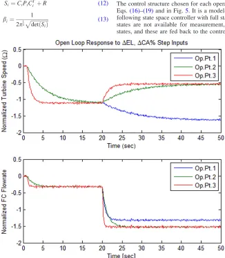
However, much research is still needed to fully understand all the aspects concerning the stability and performance of the hybrid plant. One major concern is the difference in pressure that would develop between the anode and cathode sides of the FC, when the fuel and air streams are independently controlled. This raises the question of whether it is best to control the system with a central-ized or de-centralcentral-ized controller, a linear or a nonlinear algorithm, or an adaptive control methodology [6–9]. An additional problem is the issue of compressor stall and surge due to the added volume to the compressor plenum, as well as thermal heat gradients within the FC when insufficient cathode airflow is present, or when it is in excess. It has been determined that most of these issues are directly related to the regulation of FC cathode airflow [10,11]. Hence, a thermal managing approach stemming from the routing of cathode FC airflow has been developed. The hybrid perform-ance project (HyPer) shown in Figs.1and2is a cyber-physical facility used for the study of hybrid systems [12–14]. It comprises a FC in simulation, with physical balance of plant (BoP) compo-nents that interact with the FC model in real-time. The model’s

inputs are the temperature, pressure, and mass flow rates through-out the BoP, while the model’s through-output is a calculated FC thermal exhaust that drives a fuel valve, burning natural gas. This cyber-physical approach thus allows the safe study of the dynamic cou-pling between a FC and a gas turbine GT, and the characterization of the entire operating envelope of the hybrid system, which rep-resents the main motivation behind the current study.

A unique feature of having a cyber-physical plant is the ability to derive empirical models of all the operating points of the entire system. The previous work has identified multiple operating points with the use of transfer functions [15]. These transfer func-tion (TF) matrices can be derived with ease for the entire operat-ing envelope usoperat-ing classical identification techniques, by modulating the BoP actuators, one at a time at different frequen-cies, or with the use of open-loop tests [14].

If enough models are gathered, a methodology which exploits this availability can be used to effectively control each operating point with its own independent controller. The method to identify an operating point from anNnumber of models using a statistical probability calculation is known as multiple model adaptive esti-mation (MMAE) [16–18]. Initial simulation of the MMAE algo-rithm on the HyPer BoP facility demonstrated an accurate match between an estimated model and the true system. Multiple model adaptive control (MMAC) is the extension of the MMAE algo-rithm, which includes the independent controllers for regulating the individual operating points.

The paper is divided into different sections, in the first place a description of the three operating points that were chosen to test the algorithm was presented, subsequently the MMAE approach that was used to identify the current operating point, then the MMAC methodology that describes the integration of the control-lers in one single control law.

Empirical Transfer Function Matrices

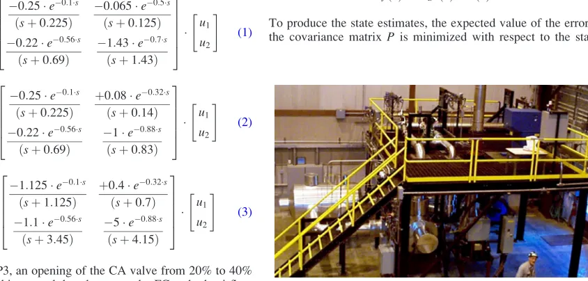
The TF matrices used in this study are those related to the cold air (CA) bypass valve and the electrical load (EL) actuation. These BoP inputs have the most weight in the thermal manage-ment of the system, and are essential to the performance and effi-ciency of the FC hybrid [7,15]. The inputs u1 and u2 in Eqs.

(1)–(3)are the EL and CA actuators, respectively, while the out-putsy1andy2are the turbine speed and FC mass flow rate. These equations provide three distinct operating points, each producing a different effect on the system response in terms of the dynamic performance, as explained in Ref. [6]. Equation (1) is the TF Manuscript received May 30, 2018; final manuscript received December 19,

2018; published online February 19, 2019. Assoc. Editor: Vittorio Verda.

The United States Government retains, and by accepting the article for publication, the publisher acknowledges that the United States Government retains, a non-exclusive, paid-up, irrevocable, worldwide license to publish or reproduce the published form of this work, or allow others to do so, for United States Government purposes.

Journal of Electrochemical Energy Conversion and Storage AUGUST 2019, Vol. 16 / 031003-1

matrix for operating point 1 (OP1), Eq.(2)for the second operat-ing point (OP2), and Eq.(3)for the third (OP3). The EL inputu1 for all three operating points is normalized with respect to its nominal operating point of 30 kW. A unit step in this actuator is equivalent to a6D20 kW change. The CA input changes between the three operating points. In OP1, the CA opens/closes from 40% to 80%, whereas in OP2 its range is from 20% to 40%. Tests have shown that the two regions exhibit a nonlinear relationship between the CA and the turbine speed, when all other parameters are held constant.

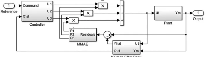
In contrast, the TF elements of OP3 (Eq.(3)) were modified to exemplify the effect no EL load would have on the turbine speed and FC mass flow rate, i.e., all the poles of the TF elements. The poles or inverse time constants were increased five times those of OP2. Figure 3 shows an open-loop step response for all three operating points. This is evidenced by the sign change in the TF element relatingy1, the turbine speed tou2, the CA valve in the following equations:

y1

y2 " #

¼

0:25e0:1s

ðsþ0:225Þ

0:065e0:5s

ðsþ0:125Þ 0:22e0:56s

ðsþ0:69Þ

1:43e0:7s

ðsþ1:43Þ

2 6 6 6 6 4 3 7 7 7 7 5 u1 u2 " # (1) y1 y2 " # ¼

0:25e0:1s

ðsþ0:225Þ

þ0:08e0:32s

ðsþ0:14Þ 0:22e0:56s

ðsþ0:69Þ

1e0:88s

ðsþ0:83Þ

2 6 6 6 6 4 3 7 7 7 7 5 u1 u2 " # (2) y1 y2 " # ¼

1:125e0:1s

ðsþ1:125Þ

þ0:4e0:32s

ðsþ0:7Þ 1:1e0:56s

ðsþ3:45Þ

5e0:88s

ðsþ4:15Þ

2 6 6 6 6 4 3 7 7 7 7 5 u1 u2 " # (3)

Note that for OP3, an opening of the CA valve from 20% to 40% increases the turbine speed, but decreases the FC cathode airflow to a larger extent, as seen in Fig.3.

Multiple-Model Adaptive Estimation

The goal of the MMAE algorithm is to assign a probability to a simulated plant model when the output of the model matches the real plant outputs in real-time. The inputs to the algorithm are the residuals, or differences between the real plant output and the out-put of a bank of Kalman filters (KF’s). The bank of KF’s, designed offline, produces an estimate of the states of all modeled operating points, when the real output signal contains measure-ment and system noise. The effectiveness of this method was shown to produce good results when the system noise is bounded [18,19]. Equations (4)and(5)show the discretized states space model for one operating point, wherew(k) andv(k) are the system and measurement noise vectors, respectively, and the cathode mass flow rate and turbine speed represent the components of the state-vector

xðkþ1Þ ¼AdxðkÞ þBduðkÞ þLwðkÞ (4)

yðkÞ ¼CdxðkÞ þvðkÞ (5)

To produce the state estimates, the expected value of the error or the covariance matrixP is minimized with respect to the states

Fig. 2 HyPer BoP test facility

(Eqs.(6)–(8)), resulting in the Kalman gainKe(Eqs.(9)and(10)), which in turn is used in Eq.(11)to calculate the estimated states^x Pðkþ1Þ ¼E½eðkþ1Þ eTðkþ1Þ (6)

eðkþ1Þ ¼xðkþ1Þ ^xðkþ1Þ (7)

Q¼diagðr2

w1;r 2

w2ÞR¼diagðr 2

v1;r 2

v2Þ (8)

Ke¼AdPCTðRþCPCTÞ

1 |fflfflfflfflfflfflfflfflfflfflffl{zfflfflfflfflfflfflfflfflfflfflffl}

H

(9)

Pi¼LQLTþAdPAdTAdPCTHCPATd (10)

^

xp¼Adx^þBduinþKeðy^yÞ

|fflfflffl{zfflfflffl} residual

^

y¼Cx^ (11)

The MMAE algorithm then uses the calculated value of the covar-iance matrix Pfrom the KF algorithm, in the computation of S

(Eq.(12)), or the covariance matrix of the residual of the error. The inverse ofSis equivalent to the variance of the sampled data, whereRis the measurement noise covariance matrix. The scalarb

is a weight attached to each probability, based on the value of_{ffiffiffiffiffiffiffi}

Si

j j

p

, which is equivalent to the standard deviation of the sampled data. In Eq.(13),Lis the number of outputs, which for our case is 2: the turbine speed and the FC mass flow rate. Given that the KF’s are built offline,P, S, andbvalues are also calcu-lated offline

Si¼CiPiCTi þR (12)

b_i¼ 1

2pL2pffiffiffiffiffiffiffiffiffiffiffiffiffiffidetð ÞS_i

(13)

PBið Þ ¼k

b_ie½12rið ÞkTSi1r1ð Þk _PB

iðk1Þ

PN j¼1

b_ie 12rjð ÞkTSj1rjð Þk

PBiðk1Þ

(14)

The final probability is given by Eq.(14), where PB is the proba-bility that system modelimatches the real output sampled data. This iterative equation is normalized by dividing the numerator by the total sum of all theNmodel probabilities. Note that the resid-ualsriare the only real-time inputs to the probability equation.

Multiple-Model Adaptive Control

Once the probabilities for each system model have been com-puted, it is an easy task to attach a control algorithm to this scheme, as shown in Fig.4. The addition of individual controllers to the MMAE approach is called MMAC. By multiplying the sys-tem model probabilities to the independent controllers designed for each individual model and then merging all the control signals into one, the outcome is an actuating control output that can be implemented for all operating points. Simply put, when the resid-uals are large, the probability is small, and the control effort for that model is small. The contribution of each controller to the total control signal is scaled by the probabilities, as shown in the below equation:

uðkÞ_T¼X

N

i¼1

uðkÞ_iPðkÞ_i (15)

The control structure chosen for each operating point is shown in Eqs.(16)–(19)and in Fig.5. It is a model-based linear reference following state space controller with full state feedback. Since the states are not available for measurement, the KF estimates the states, and these are fed back to the controller. Figure5does not

Fig. 3 Open-loop response for three operating points

show the KF subsystem. In Eqs.(17)and(18),Adis the discrete transmission matrix,Bdis the input matrix, andCdis the output matrix [20,21]. The state feedback matrixKin Eq.(18)is calcu-lated with the use of the pole placement design, where the desired closed-loop polesbare assigned according to a specified dynamic performance, i.e., percent overshoot to a step input and settling time

uðkÞ_i¼ðNuþKiNxÞ rKi^xi (16)

Nx

Nu

¼ AdI Bd

Cd 0

1

0

I (17) zIAdþBdK

j j ¼0 (18)

zi¼b1;b2;…;bn (19)

In order to simulate a sequential changing of operating points in

SIMULINK, a logical subsystem shown in Fig.6was developed to

switch between plants at various time intervals. By using else-if

action subsystems activated with logical gates which are fed by time threshold inequalities, the MMAC algorithm can be tested for a known set of sequential events. Each subsystem in Fig.6 represents a TF matrix of Eqs.(1)–(3). The fourth subsystem is one of the three OP repeated.

As previously stated, a bank of KF’s is designed offline for each of the three operating points analyzed. Figure 7shows the bank used, each receiving the measured outputYand the overall control signalU. The output is an estimated state ^xand an esti-mated outputy^. Figure8shows the prediction type KF (PTKF) used, highlighted in yellow.

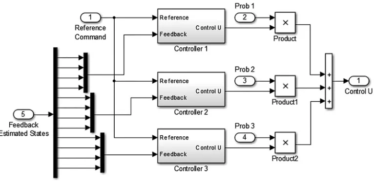
Figure9shows theSIMULINKcontroller subsystem, having each

block follow the architecture of Fig.5. The output of each control-ler block is multiplied by the probability corresponding to the model the controller is designed for. The total control signal is thus the addition of all control efforts scaled by their respective model probabilities.

The final component to the MMAC algorithm is the probability function described by Eq.(14). Figure10shows theSIMULINK

rep-resentation of Eq.(14)with residual inputs.

Fig. 4 Multiple model adaptive controlSIMULINKmodel

Fig. 5 Model of the full state feedback reference controller [2]

Fig. 7 SIMULINKKF bank subsystem

Fig. 8 Prediction type KFSIMULINKsubsystem

Fig. 9 SIMULINKcontroller subsystem

Fig. 10 Probability equation in aSIMULINKsubsystem

Results

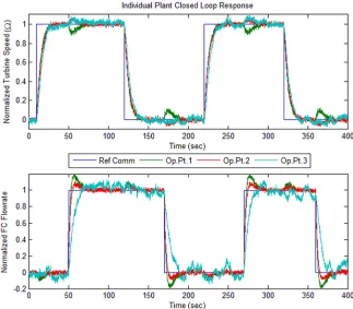
Figure11shows the closed-loop response of each of the three individual TF matrices to a normalized step input, using the con-trol law of Fig.5. This response does not represent the multiple model arrangement, but rather a single input/single output system used to validate the individual controller performance. All designed controllers follow the pole placement methodology.

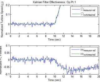
Figure12illustrates the effectiveness of the KF estimate, for a noisy turbine speed and FC airflow measurement signal inputs.

Since the steady-state KF’s are all designed offline Eqs.(9)and (10), the computational burden of inverting matrices in real-time is removed, allowing for a faster implementation of the MMAC algorithm, i.e., Eq.(11)is the only equation implemented online.

To understand the importance of having an individual controller designed for a specific operating point, the actuator response of the two OP’s of the CA bypass valve is displayed in Fig.13, for the correct control assignment, i.e., for a well-matched controller to plant pairing. It is evident that in order for the turbine speed and FC cathode airflow to follow the reference commands of

Fig. 12 KF estimation effectiveness

Fig. 13 Actuator CL response comparison for OP1 and OP2

Fig.11, a different EL is required when the CA is in the 40–80% range (OP1) than when it is in the 20–40% lower range (OP2). A closer look at Fig.11shows that between 50 and 120 s, the times in which a reference command for FC flow and turbine speed are set, the EL changes direction in Fig.13. This is also the case when a separate reference command is set between 270 s and 320 s.

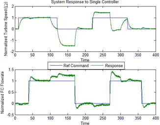
To further demonstrate the detrimental effect a linear controller designed for a single operating point would have on other operat-ing points, the multiple model switchoperat-ing logic of Fig. 6 was applied to the controller for OP1. The response of Fig.14shows the controller’s inability to follow reference commands when the

plant changes at 100 s, 150 s, and 300 s. To scale the response of this figure, the turbine speed is multiplied by 500, and the nominal value of 40,500 rpm added. To scale the FC mass flow rate to actual values, the number is multiplied by 0.2 kg/s and its nominal value of 1.7 kg/s added.

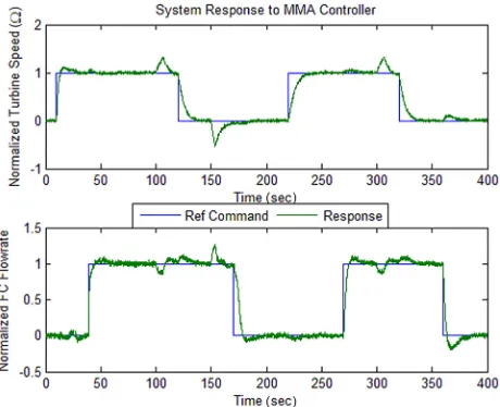
In contrast to Fig.14, Fig.15shows the response of the system to the MMAC algorithm, when the plant changes from OP1–OP2–OP3–OP1 at time intervals 0 s, 100 s, 150 s, and 300 s. It is clearly seen that the controller response in tracking the refer-ence command signal is greatly improved from the response of Fig. 14. Although an over- and under-shoot transients are still

Fig. 14 Single controller response for multiple plant changes

present at the moment of system change, the recovery is nonethe-less achieved at an acceptable pace in accordance with the conver-gence time of the MMAC algorithm.

The closed-loop EL and CA actuator response is shown in Fig.16. Compared to the actuator response of Fig.13when OP1 and OP2 are separately controlled, the EL load of Fig.16 fluctu-ates intermittently between the behavior observed in OP1 and that of OP2. Hence, having two different controllers operating at the same OP, produce an opposite response in the EL load. Since the final control signal is composed of all the individual control sig-nals weighted by their respective model probabilities, the MMAC is able to track the command well, even in the face of the nonli-nearity. The actuator signals are bounded within the allowed limits.

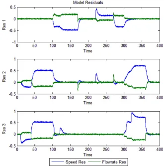
Figure 17 shows the model residuals for each OP. There are two residuals per OP—one for the estimated versus real turbine speed and the other for the estimated and real FC cathode airflow. In the simulation, the lower residuals indicate a match between estimated and true values, indicating a greater probability assigned to that particular model. As expected, the residuals fol-low the sequence of system plant changes designated as OP1–OP2–OP3–OP1. The closeness of the residuals between regions of plant change 2–3 are a result of the similarity the TF matrices have. Note that the third OP was built according to the second OP, but with a faster response, i.e., faster poles or time constants.

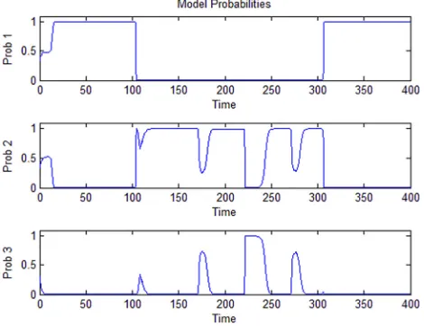
Figure 18shows the probabilities of the models, according to the system plant change sequence OP1-2-3-1. The graph demon-strates that from the initial 1/3 probability each model has, the MMAE algorithm correctly converges to a probability of 1 for OP1 up to 100 s, when the true plant was switched. After 100 s, OP2 is switched and the estimation outputs a probability of 1 for model 2. The third OP is then switched between 150 s and 300 s after which OP1 is switched again until the end of the simulation. The noticeable spikes between the probabilities of OP2 and OP3 indicate a convergence difficulty when the residuals are similar, as noted in Fig.17. This is expected, since the model for OP3 was based on the model of OP2, i.e., OP3 is OP2 with faster poles. Even with the convergence discrepancy, the robustness of the con-troller is validated in Fig.15.

To further validate the MMAC method, a second sequence of plant changes was performed, as shown in Figs. 19–22. In this instance, the sequence of operating points was OP3–OP1–OP2–OP1.

As with the previous sequence of plant switches, the probabil-ities correctly match a model to the particular plant output, with

Fig. 16 Actuator CL response of the MMAC

Fig. 17 Multiple model adaptive estimation calculated residuals for the three OP’s

similar discrepancies between OP2 and OP3. The times of the sec-ond sequence are the same as the time for sequence no. 1. The MMAC controller is still able to manage a better response from that observed in Fig.14.

Discussion

The previous graphs demonstrate the performance and limita-tions of the MMAC methodology. One very important advantage of the MMAC is the ability for this algorithm to merge various controllers into one signal by scaling each control component with a probability weight. This is ideal for highly nonlinear sys-tems, where no two controllers are alike. In this study, the pole placement approach was used for all three OP’s, but could have easily had incorporated an entirely different control scheme. If for example, the startup of the hybrid system can benefit from opera-tor expertise, a fuzzy logic controller can be designed for this OP. If on the other hand, a robust and safe shutdown is desired, an optimalH1can be implemented. The ease of control switching is

only restricted by the convergence of the adaptive estimation. As is the case with all control algorithms, there are disadvan-tages to the MMAC which can result in undesired responses. A notable problem arises when the OP’s are similar and have static gains which are close to each other. This was the case for models 2 and 3. A close look at Eqs.(2)and(3)reveals that the only dif-ference between these TF matrices is the speed of the response. All the poles of the TF elements are modified to be five times

faster. The apparent change in static gain is only the result of the mathematical manipulation of increasing the value of the poles. As can be seen in Fig.3, the steady-state gain for both OP2 and OP3 is the same, only that OP3 is faster. The result of having sim-ilar parameters between OP’s is the difficulty for the MMAE to converge to one specific probability model, given that the resid-uals are almost identical. This can be observed in Figs.18and21, at the times when the probabilities experience “noise.”

Convergence is also dependent upon whether the models are spaced at regular intervals. This is reflected in the b parameter which in turn relates to the variance of the sampled dataSmatrix. When all the modelbare similar, no OP “dominates” with respect to how distant it is from the rest of the OP’s. Thebvalues for all three OP’s were found to be within 1–7% of each other, allowing for a satisfactory convergence, apart from the residual issue.

From Figs.17and20, the residual effect of OP2 and OP3 can also be inferred in the EL and CA actuators. Both actuators show a smoother trend when OP1 is encountered. Small ripples are present during the OP2 and OP3 plant switches. This can be seen at times prior to 50 s in Fig. 23 where OP3 is present, as well as in time 150 s, when OP2 is assigned. A similar trend is shown in Fig.17.

With regard to the practical implementation of the MMAC algorithm, it is best to utilize actuators with enough bandwidth to be able to reduce the system noise. The previous work confirmed the difficulty in convergence when the system noise is increased, as opposed to the measurement noise of the sensors [2]. It is thus essential to diminish plant disturbances stemming from faulty or degrading actuators. The covariance matricesQandRused in this study had scaled down values in accordance with the normaliza-tion of the turbine speed and FC airflow signals. An increase in theQmatrix diagonal elements will result in a noisier probability plot.

A minor, but important detail comes with the implementation of the probability function of Eq.(14). Given that the denominator is used to normalize the calculated value to be a number between 0 and 1, none of the probabilities can ever reach zero. A smalle

value is added to all probabilities to account for the otherwise division by zero.

Finally, the use of the MMAC methodology can be extended to controlling the FC-GT hybrid in the presence of disturbances, as is the case with sudden increases in load requirements. By adding a controller to mitigate disturbances when these are detected by the MMAE estimation algorithm, a more robust system can be achieved. These disturbances might actually cause a more drastic

Fig. 18 Model probabilities for the response in Fig.16

change in the system dynamics than the one shown by the influ-ence of the CA bypass valve. The MMAE not only is useful for OP matching, but also for sensor failure detection, as noted in Ref. [2].

Conclusions

The MMAC methodology was proven to be a relevant and fea-sible control algorithm in the hybrid performance system, given its ability to simultaneously operate plant actuators with a variety of control strategies. The strong coupling of the FC-GT system requires a controller to be flexible and adaptive to changing oper-ating conditions. Having a control strategy that is able to merge various control algorithms into one is ideal for the nonlinear oper-ating envelope. With MMAC, the benefit of linear and nonlinear controllers can thus be exploited, reducing the control issues asso-ciated with hybrid plants.

Acknowledgment

This work was completed through a collaboration between the U.S. Department of Energy Crosscutting Research Program, administered through the National Energy Technology Labora-tory, Ames LaboraLabora-tory, and the U.S. Coast Guard Academy.

Nomenclature

A¼state matrix

B¼input matrix

C¼output matrix

e¼error between the estimated state and the state vector

E¼expected value of the error

k¼discrete time variable

Ke¼Kalman gains

L¼process noise matrix

P¼covariance matrix

Q¼process covariance matrix

s¼Laplace variable

u¼inputs

v¼measurement noise vector

w¼process noise vector

x¼state vector

^

x¼state vector estimation

y¼outputs

References

[1] Tucker, D., Lawson, L., and Gemmen, R., 2003, “Preliminary Results of a Cold Flow Test in a Fuel Cell Gas Turbine Hybrid Simulation Facility,”ASME

Paper No. GT2003-38460.

[2] Tucker, D., Liese, E., and Gemmen, R., 2009, “Determination of the Operating Envelope for a Direct Fired Fuel Cell Turbine Hybrid Using Hardware Based Simulation,” International Colloquium on Environmentally Preferred Advanced Power Generation, Newport Beach, CA, Feb. 10–12, Paper No. ICEPAG2009-1021.

[3] Tucker, D., and Gemmen, L. Lawson, R., 2005, “Characterization of Air Flow Management and Control in a Fuel Cell Turbine Hybrid Power System Using Hardware Simulation,”ASMEPaper No. PWR2005-50127.

[4] Winkler, W., Nehter, P., Tucker, D., Williams, M., and Gemmen, R., 2006, “General Fuel Cell Hybrid Synergies and Hybrid System Testing Status,”J. Power Sources,159(1), pp. 656–666.

[5] Williams, M. C., Strakey, J., and Surdoval, W., 2006, “U.S. DOE Fossil Energy Fuel Cells Program,”J. Power Sources,159(2), pp. 1241–1247.

[6] Pezzini, P., Banta, L., Traverso, A., and Tucker, D., 2014, “Decentralized Con-trol Strategy for Fuel Cell Turbine Hybrid Systems,” 57th Annual ISA Power Industry Division Symposium, Scottsdale, AZ, June 1–6, Paper No. POWID2014-52.

[7] Pezzini, P., Celestin, S., and Tucker, D., 2015, “Control Impacts of Cold-Air Bypass on Pressurized Fuel Cell Turbine Hybrids,”ASME J. Fuel Cell Sci. Technol.,12(1), p. 011006.

[8] Tsai, A., Banta, L., Tucker, D., and Gemmen, R., 2010, “Multivariable Robust Control of a Simulated Hybrid Solid Oxide Fuel Cell Gas Turbine Plant,”

ASME J. Fuel Cell Sci. Technol.,7(4), p. 041008.

[9] Tsai, A., Tucker, D., and Groves, C., 2010, “Improved Controller Performance of Selected Hybrid SOFC-GT Plant Signals Based on Practical Control Schemes,”ASME J. Eng. Gas Turbines Power,133(7), p. 071702.

[10] Tucker, D., Lawson, L., Smith, T., and Haynes, C., 2006, “Evaluation of Cathodic Air Flow Transients in a Hybrid System Using Hardware Simulation,”

ASMEPaper No. FUELCELL2006-97107.

[11] Tucker, D., Ford, J., Haynes, C., VanOsdol, J., Liese, E., and Lawson, L., 2012, “Evaluation of Methods for Thermal Management in a Coal Based SOFC Tur-bine Hybrid Through Numerical Simulation,”ASME J. Fuel Cell Sci. Technol., 9(4), p. 041004.

[12] Traverso, A., Tucker, D., and Haynes, C., 2012, “Preliminary Experimental Results of Integrated Gasification Fuel Cell Operation Using Hardware Simu-lation,”ASME J. Eng. Gas Turbines Power,134(7), p. 071701.

[13] Tucker, D., Smith, T., and Lawson, L., 2006, “Characterization of Bypass Con-trol Methods in a Coal Based Fuel Cell Turbine Hybrid,” ASME Paper No. ICEPAG2006-24008.

[14] Zhou, N., Yang, C., Tucker, D., Pezzini, P., and Traverso, A., 2005, “Transfer Function Development for Control of a Fuel Cell Turbine Hybrid System,”Int. J. Hydrogen Energy,40(4), pp. 1967–1979.

[15] Tsai, A., Banta, L., Tucker, D., and Lawson, L., 2009, “Determination of an Empirical Transfer Function of a Solid Oxide Fuel Cell Gas Turbine Hybrid System Via Frequency Response Analysis,”ASME J. Fuel Cell Sci. Technol., 6(3), p. 034505.

[16] Chang, C., and Athans, M., 1978, “State Estimation for Discrete Systems With Switching Parameters,”IEEE Trans. Aerosp. Electron. Syst.,AES-14(3), pp. 418–425.

[17] Narendra, K. S., and Xiang, C., 2000, “Adaptive Control of Discrete-Time Sys-tems Using Multiple Models,” IEEE Trans. Autom. Control, 45(9), pp. 1669–1686.

[18] Athans, M., 1977, “The Stochastic Control of the F-8C Aircraft Using a Multi-ple Model Adaptive Control (MMAC) Method—Part I: Equilibrium Flight,”

IEEE Trans. Autom. Control,AC-22(5), pp. 768–780.

[19] Tsai, A., Tucker, D., and Emami, T., 2016, “Multiple Model Adaptive Estima-tion of a Hybrid Solid Oxide Fuel Cell Gas Turbine Plant Simulator,”ASME

Paper No. FUELCELL2016-59656.

[20] Lewis, F., 1992,Applied Optimal Control and Estimation, Digital Design and Implementation, Prentice Hall, Englewood Cliff, NJ.

[21] Franklin, G. F., Powell, J. D., and Workman, M. L., 1998,Digital Control of Dynamic Systems, 3rd ed., Addison Wesley Longman, Inc., Menlo Park, CA.

Fig. 21 Closed-loop response of sequence no. 2

Fig. 22 Actuator response for sequence no. 2