University of New Orleans University of New Orleans
ScholarWorks@UNO
ScholarWorks@UNO
University of New Orleans Theses and
Dissertations Dissertations and Theses
12-15-2007
On the Determination of Building Footprints from LIDAR Data
On the Determination of Building Footprints from LIDAR Data
Henry C. George
University of New Orleans
Follow this and additional works at: https://scholarworks.uno.edu/td
Recommended Citation Recommended Citation
George, Henry C., "On the Determination of Building Footprints from LIDAR Data" (2007). University of New Orleans Theses and Dissertations. 605.
https://scholarworks.uno.edu/td/605
This Thesis is protected by copyright and/or related rights. It has been brought to you by ScholarWorks@UNO with permission from the rights-holder(s). You are free to use this Thesis in any way that is permitted by the copyright and related rights legislation that applies to your use. For other uses you need to obtain permission from the rights-holder(s) directly, unless additional rights are indicated by a Creative Commons license in the record and/or on the work itself.
On the Determination of Building Footprints from LIDAR Data
A Thesis
Submitted to the Graduate Faculty of the University of New Orleans in partial fulfillment of the requirements for the degree of
Master of Science in
Engineering Electrical Engineering
by
Henry C. George
B.S. University of New Orleans, 2005 M.S. University of New Orleans, 2007
Acknowledgements
The research was supported by NASA as part of an SBIR project with collaboration provided by Diamond Data Systems and UNO. Thanks were given to major professor Dr. Dimitrios
Charalampidis for his help and to Dr. Huimin Chen and Dr. Vesselin Jilkov for serving as thesis committee members and for their helpful comments. Special thanks were given to my family for their support.
iii
Table of Contents
List of Figures ... iii
Abstract ... iv
Chapter 1...1
Introduction to LIDAR ...1
The LIDAR Collection Process ...1
LIDAR Data...2
Chapter 2...3
LIDAR Processing Applications...3
Creation of Digital Elevation Models ...3
Building Identification and Modeling...4
Chapter 3...5
Building Footprint Extraction ...5
Pre-Processing Techniques ...5
The Progressive Morphological Filter ...7
The Region Growing Algorithm...9
Plane-Fitting Techniques ...15
Merging of Building Surfaces...17
Building Footprint Post-Processing ...18
The Douglas-Peucker Algorithm ...18
Chapter 4...21
Region Growing Algorithm Improvements ...21
Boundary Point Identification...21
Boundary Point Region Growing...22
Satellite Image Processing ...23
Chapter 5...26
Comparative Results ...26
Conclusions...27
Future Work ...27
References...28
List of Figures
Figure 1: Aircraft Emitting Laser Pulses for LIDAR Collection...2
Figure 2: Mount Saint Helens Digital Elevation Model ...3
Figure 3: Pre-Processed LIDAR Image After Interpolation ...6
Figure 4: Grayscale Image After Morphological Processing ...9
Figure 5: Region Growing – A Graphical Example ...10
Figure 6: Region Growing – Example After Multiple Iterations...10
Figure 7: Inside Point Region Identification...14
Figure 8: Boundary Point Region Identification...14
Figure 9: Visualizing the Douglas-Peucker Algorithm ...19
Figure 10: Douglas-Peucker Algorithm Resulting Image ...20
Figure 11: Boundary Point Region Identification – New Definition...21
Figure 12: Douglas-Peucker Algorithm – Improved Sort...23
Figure 13: Satellite Image Data ...24
Figure 14: Boundary Point Identification – Comparison...26
Figure 15: Douglas-Peucker Algorithm – Comparison ...26
v Abstract
A new approach to improve the determination of building boundaries through automatic processing of light detection and ranging (LIDAR) data is presented. The LIDAR data is processed and interpolated into a grayscale image of intensity values corresponding to height measurements. Ground measurements are separated from non-ground measurements by using a progressive morphological filter. With these measurements now distinct, further separation of non-ground measurements into building and non-building measurements is performed by
growing regions with similar characteristics. These building areas are then refined, resulting in a ground plan representation of building boundaries, known as building footprints. Several
algorithms are then implemented to clean these footprints. A new method is developed to analyze actual known satellite imagery in order to confirm identified building footprints.
Chapter 1
Introduction to LIDAR
Light detection and ranging (LIDAR) is an application of lasers used to discover information about a distant object, usually some form of distance information. LIDAR data are usually collected via airplane, with the airplane traversing a subject area of interest and collecting data about this area through the use of laser pulses. These laser pulses are emitted from the airplane fuselage from a laser scanner device, and the round trip travel time from this emission and the returning light is measured. This time delay is then used to determine the elevation of the ground in this particular area. LIDAR equipment is usually paired with a global positioning system (GPS) in order to accurately pinpoint the x and y coordinates of a specific data measurement.
The LIDAR Collection Process
The way in which LIDAR data is collected is a very detailed one that needs to be explained more thoroughly in order to appreciate it fully. This information as released by the National Oceanic and Atmospheric Administration (NOAA) details in depth about how this data is so intricately extracted. Already discussed is the use of laser pulses, which scan the area of interest up to 5000 pulses per second.
The laser type used is generally the neodymium-doped yttrium aluminum garnet (Nd:YAG) laser with a wavelength around 1064 nanometers, placing the laser in the infrared range of light. This pulsed laser is emitted when the population inversion in the resonator has reached its maximum, achieved by what is known as Q-switching, which places a switch inside the resonator which releases the stored pulse when the maximum amount of atoms are in an excited state.
Of major interest is the mechanism which allows this technology to perform its task of collecting LIDAR data. Two mirrors, one a 45-degree angled folding mirror and the other a moving
mirror, combine to direct the laser pulses towards the ground. The laser pulses encounter the folding mirror first, with the reflection directed towards the moving mirror below. The reflection from the moving mirror directs the laser pulses towards the ground, with an overall coverage angle of 30 degrees. Since these aircraft fly at heights of around 700 meters, the 30 degree angle allows an overall circular coverage area with a diameter of approximately 350 meters.
2
Figure 1: Aircraft Emitting Laser Pulses for LIDAR Collection
LIDAR Data
With the LIDAR data collected, the real question becomes apparent: how is LIDAR data processed? LIDAR data in combination with a GPS allow for each measured elevation to be paired with its location, effectively creating a three-dimensional coordinate for each measured elevation. The x and y coordinates are usually latitudes and longitudes derived from the GPS system, while the z coordinate is the measured elevation using the LIDAR collection device, measured usually in either meters or feet. An ASCII file with each line containing a
Chapter 2
LIDAR Processing Applications
LIDAR data is currently being used in a diverse array of applications, ranging from the study of seismology to traffic control analysis. LIDAR is used in seismology to detect faults, with one such example relating to a particular fault in Seattle. LIDAR allowed the detection of the Seattle fault from an earthquake that occurred over 1000 years ago, effectively painting a picture of the surface in the area by penetrating through tree canopies, allowing for a view of what is now known as the Seattle fault. LIDAR data is also used in traffic law enforcement, replacing radar as a speed detector in police laser systems. Other applications of LIDAR relate to its use in adaptive cruise control systems in cars and its use as a height measuring tool in the forestry industry.
One of the main uses of LIDAR data and an important idea in the development and identification of building footprints pertains to its ability to create topographic maps of areas. LIDAR data is able to be manipulated and processed in such a way to allow a visual representation of an area based on the time delay measurements translated into heights along with the paired GPS coordinates. The final result of such processing techniques on this data is known as a digital elevation model (DEM).
Creation of Digital Elevation Models
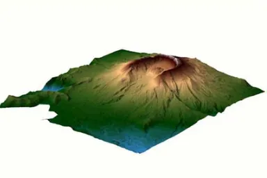
While the creation of DEMs is not directly considered here, it is important to note its use as it is the main scientific and image processing based application of LIDAR data. In the figure below, a DEM of Mount Saint Helens is shown as an example of this particular LIDAR application performed by LIDAR mapping company EarthData [9].
Figure 2: Mount Saint Helens Digital Elevation Model
4
LIDAR intensity images are also an important visualization of LIDAR data, allowing irregularly spaced LIDAR data to be represented as a digital grayscale image of varying intensities, with higher intensities representing higher elevations, and lower intensities representing lower
intensities. This particular creation of grayscale intensity images will prove extremely important in the classification of particular areas of interest, in this case, the classification of buildings.
Building Identification and Modeling
LIDAR intensity images can be examined using image processing techniques. These techniques allow the visual representation of LIDAR data to be identified, classified, and separated into areas of interest to be analyzed. One such classification involves the identification of buildings, with this identification proving important in various real life applications, including the study of urban population and the development of ground plans. The identification of buildings can also be extended into the development of three-dimensional building models.
Previous work has successfully identified building footprints through the use of filtering, region growing, and dominant direction estimation [1]. However, the use of dominant direction estimation as a means of cleaning building footprints assumes a particular relationship between perpendicular/parallel building edges and oblique building edges. Also, a visual comparison to aerial imagery was used to detect omission and commission errors. With a refined definition of what constitutes a building boundary along with a new method for confirming building
Chapter 3
Building Footprint Extraction
One of the major applications of LIDAR technology has been the ability to use the data for feature extraction and identification. Building footprint extraction is just one of the many feature extraction opportunities provided by airborne LIDAR data. The goal is to determine the location of buildings in the area of interest, effectively separating buildings by determining their
boundary. There are many ways to accomplish this task, with commonalities along the way in each. One such method of extracting building footprints will be described in great detail here.
Pre-Processing Techniques
Before any analysis can be done on LIDAR data, the data must become useful in a way that allows understanding and interaction. Once the area of interest has been determined, the LIDAR XYZ files need to be interpreted in a way to allow such an understanding to be possible. A visual depiction of LIDAR data becomes a necessary means for understanding and future analysis, and the use of image processing provides such a means to the researcher. The LIDAR data will be visualized in a digital image, with the x and y values representing pixel coordinates of the image, and the elevation value z representing the intensity value of the grayscale image. This pre-processing stage sets up the ability for any application of LIDAR data and will help to extract building footprints.
First, the LIDAR data XYZ files are read into a three-dimensional array, with each coordinate (x,y,z) being read into a row of the array. The goal is to create an image using the LIDAR data points that maps each coordinate to a pixel or group of pixels. LIDAR data by its very nature has a randomness to its data points, which prohibits a one-to-one mapping of each LIDAR point to a pixel, as some areas have such a dense coverage but others are sparsely sampled. Upon reading the data into the array, the number of points read is determined and stored in order to find the minimum x and y values of the LIDAR data. The horizontal size of the image is determined by the user, and the vertical size is derived based on this horizontal size by manipulation of the maximum and minimum coordinates, as indicated in the following equation.
) min( ) max( ) min( ) max( y y x x width height − − ×
= (1)
Basically, the user controls how large of an image the LIDAR data will be processed into, but only to an extent. The LIDAR data itself and its range determines the height to prohibit too small or too large an overall image size chosen. However, this can result in some information loss because of the lack of a one-to-one mapping as stated above. Also, each pixel could contain more than one LIDAR coordinate point, in which case the smallest elevation value is chosen as the pixel value at that location. This would seem to grid the LIDAR data into an image
6
Once the above step is performed, the image is processed further by interpolation of pixel values. The image is interpolated in order to replace the place holder points described above with a minimum elevation value in a window. A window size w is specified for this interpolation with a value of 3. Each pixel value is scanned in a search for the place holder value, indicating that there is no data for this specific location in the area of interest. When a pixel of this value is found, the pixel values in the window are scanned. If less than 25% of the pixel values in the window contain the place holder value, the minimum pixel value in the window is determined and assigned to the pixel in question. However, if more than 25% of the pixel values in this window also contain the place holder value, then the pixel value in question remains the place holder value, but the window size is increased by two. This process continues up to a maximum window size specified by the user, in this case the maximum window size being 15. This
progressive window operation allows stray place holder pixels to be replaced by surrounding values in order to have a more complete image, but place holder pixels that do not get replaced through this interpolation remain as such and are represented in the resulting pre-processed grayscale image as the highest intensity possible, resulting in a white color. The resulting image after interpolation is shown in Figure 3 below.
Figure 3: Pre-Processed LIDAR Image After Interpolation
This image represents a subset of Lenoir County, North Carolina. The pre-processed image above is of size 1201x401, obtained through the interpolation methods discussed above. Upon examination of this final pre-processed image, a few traits are immediately noticeable. First, the portions of the image that had no LIDAR data points corresponding to the actual pixel coordinate have a white intensity. Also, the overall intensity differences, ranging from light grey to a
grayscale intensity that is close to black in color, indicate elevation differences of the LIDAR data coverage area. The lower intensities (dark grey / black) represent very low-lying areas
relative to the rest of the coverage area, indicating that these points are most likely ground points. The higher intensities (lighter grey) indicate that the elevation is higher in those locations and could therefore correspond to buildings, but further detail will be necessary to make such a determination. This pre-processed image represents the starting point for all further analysis, as various image processing techniques will be employed in order to accomplish the task of
The Progressive Morphological Filter
With the pre-processed image obtained, and the overall goal being to determine the locations of buildings and their boundaries, a method must be determined to perform such a separation of the building pixels from the rest of the image. However, one cannot simply separate the building objects from the rest of the image immediately. First, the pixels representing ground elevations must be separated from the pixels representing non-ground elevations. Non-ground elevations refer to any pixel whose intensity has a value greater than a predefined threshold for height, regardless of whether or not the point corresponds to a building, vegetation, or other object that is higher off the ground than this predefined threshold.
There are many methods that have been employed in order to accomplish this task of separating non-ground points from ground points. One such way was formulated by Vosselman, who identified non-ground points and separated them from ground points by analyzing the slope between a given pixel and the eight neighbors of the pixel. Vosselman determined the slope from a given pixel to each of its neighbors, and then found the overall maximum slope. If the maximum slope was less than a predefined threshold, then the point was labeled a ground point; otherwise, the point was considered a non-ground point.
The major pitfall with separating non-ground points from ground points arises in the derivation of a best-fit filtering threshold. Zhang [2] has identified the following two general problems with separating ground points from non-ground points: commission errors and omission errors. Commission errors refer to mistakenly identifying non-ground points as ground points, while omission errors refer to mistakenly including ground points as non-ground points. If one selects the best-fit threshold for the filtering method of choice, then these errors will be minimized, and the resulting separation will be as accurate as possible. Zhang proposed what is known as the progressive morphological filter to mathematically remove non-ground points from a processed grayscale image like the one in Figure 3 above.
A morphological filter is a filter that utilizes a combination of dilations and erosions in order to dilate and/or erode features of an image. When dealing with a grayscale image as in the pre-processed image of Figure 3, these dilation and erosion operations actually become maximum and minimum operations. The progressive morphological filter combines the use of maximum filters and minimum filters in order to detect the non-ground elevations by effectively replacing all of these values with ground pixel values, removing the non-ground pixels from the image.
8
combination of a minimum filter following by a maximum filter is known as an opening operation of the morphological filter.
Once this initial opening operation is performed, the difference between the original image and the new image filtered using the opening operation is obtained. This image should therefore have pixel intensity values of zero for all ground pixels since the ground pixels were not removed in the opening operation performed. However, this image should have pixel values relating to the non-ground values in the original image, as the difference image was obtained by subtracting each intensity value of the filtered image from the original image. This difference image now becomes extremely important in the implementation of the progressive
morphological filter as it relates directly the best-fit threshold described above. The height threshold was predefined to be 0.1 for this morphological operation. However, the best-fit threshold was determined to be dependent on the window size in the following way:
threshold height
w threshold morph
best_ _ = × _ (2)
Therefore, the actual filtering operation occurs by comparing each difference image pixel value with this best-fit threshold value. If the given difference image pixel value is greater than this best-fit threshold value, then the corresponding original pixel value is replaced with the pixel value of the image obtained after the opening operation. If the given difference image pixel value is less than the best-fit threshold value, then the corresponding original pixel value remains the same. This process repeats every pixel of the image is traversed.
Upon initial viewing, one would think that the operation performed in equation (2) would simply set the best-fit threshold to a value of 0.3 since the window size above was chosen to be three. However, this is not the case, as this morphological operation is progressive in nature. The progressive nature of the morphological filter refers to the fact that the window size progresses to a higher value after each performance of this algorithm. A maximum window size is set by the user initially. A window step size is also set initially by the user, which indicates how much the window will increase after each traversal of the algorithm. In this particular case, a maximum window size of 40 and a window step size of 10 were chosen. The following table shows the progressive increasing nature of the window size for the morphological filtering operation.
Table 1: Progressive Morphological Filter Window Sizes
# of Executions Window Size (w) Best Fit Threshold
1 3 0.3
2 13 1.3
3 23 2.3
4 33 3.3
operation. This process is repeated until the maximum window size of 40 was achieved. The best-fit threshold also progressively changes with respect to the window size according to equation (2) above. The grayscale image obtained after removal of all non-ground objects through the implementation of the progressive morphological filter is given in Figure 4 below.
Figure 4: Grayscale Image After Morphological Processing
In comparison to the original pre-processed image in Figure 3, one can see that the areas of higher intensity are now completely removed in Figure 4. This proves that the progressive morphological filter performed well in separating ground pixel values from non-ground pixel values.
The Region Growing Algorithm
With the non-ground pixel values successfully separated from the ground pixel values and identified, the algorithm to identify building areas and their boundaries becomes the focus. The algorithm proposed to accomplish the task of separating building areas from other non-building non-ground objects is the region growing algorithm. The region growing process will iteratively separate the non-ground pixels into distinct regions of interest which will allow a successful building footprint extraction.
10
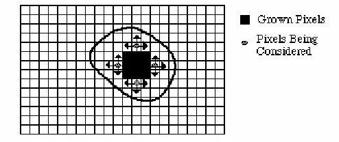
Figure 5: Region Growing - A Graphical Example
The seed pixel is the first pixel in the scanned image containing a “true” output to the testing condition. The region will then grow outward from this pixel by testing each of the pixels eight neighbors individually, adding said pixels to the region if the condition is satisfied. Figure 6 below illustrates the region growing process after multiple iterations of the condition check.
Figure 6: Region Growing – Example After Multiple Iterations
As can easily be seen, the highlighted area in the above figure indicates that these particular pixels satisfied the condition for inclusion and therefore are now members of the region. This process continues until no new neighboring pixels can be added to the region, creating an effective boundary for the region in question.
With the basics of the region growing process now explained, the detailed region-growing algorithm applied to the specific Lenoir County area of North Carolina is performed. The progressive morphological filter has effectively separated the ground and non-ground pixels by creating an output image that has removed all non-ground pixels and replaced them with average ground pixel values.
is a set of regions of inside points, along with a set of regions of boundary points corresponding to these inside point regions.
The region growing process for segmenting regions of inside points is the first task after the progressive morphological filtering operation is performed. First, a testing condition must be established which will allow for a new region to begin from an initial seed point with properties that satisfy the condition. A height (pixel intensity value) threshold is chosen as this initial condition, given a value of 10, and this threshold will be the first testing condition upon which a region is initiated. This threshold is variable, allowing the algorithm to run with any threshold with value greater than zero desired. The image to be operated on is the difference image, which now contains intensity values near zero for ground pixels and intensity values equal to the height of non-ground objects for all pixels that are not considered part of the ground area. The
difference image is scanned, starting from the upper left corner, until a pixel with intensity value greater than the threshold is found. This initial conditioning does not identify the point as an inside point, so the pixel cannot yet be added to a region.
Once a pixel satisfying the initial threshold condition is found, further conditioning is performed to determine whether or not this pixel is an inside point. Of note is the fact that each pixel will be identified as “belonging to a region” or “not belonging to a region” by a labeling scheme within the algorithm itself. Initially, all pixels will contain a label of “not belonging to a region.” The second condition tests whether the pixel belongs to a region already by scanning the pixel’s label for this information, represented in the algorithm as a Boolean ‘1’ (belongs to a region) or ‘0’ (does not belong to any region). If the pixel does not belong to any region as of yet, the second condition is satisfied and further conditioning is performed. The third and final condition does not test the pixel in question itself, but the pixel’s eight neighbors. The third condition checks whether all of the eight neighbors satisfy the initial condition of having an intensity value greater than the threshold. This is accomplished by performing an AND operation of each neighbor condition, resulting in a satisfied condition only when all pixels are greater than the threshold. If all of the eight neighboring pixels have a value greater than this threshold, then the pixel in question is indeed an inside point. Therefore, the pixel is added to the region as the seed point and labeled as described above as “belonging to a region” to avoid placing the same pixel in multiple regions or in the same region more than once. The pixel is added to the region in the algorithm itself by utilizing linked lists, with each region being identified by its own linked list. This allows for each region to have varying size along with the possibility of adding pixels at a random rate based on condition testing. If the above process fails to produce a pixel that satisfies the conditions of an inside point, the difference image scan continues until the first inside point is found, making it the initial seed point for the region.
With the seed point for the inside point region determined, the region must then be grown. Since a seed inside point was found, the scanning of the difference image stops. The location of the scan is saved so that when the region is completely grown, the scan can begin again from the same location, looking for another region to grow. As shown in Figure 5 above, the region growing process grows outward from the seed point, so the conditioning moves on to the eight neighbors of the seed point.
12
passes the initial threshold test. Therefore, the upper-left neighbor is tested based on whether or not it already belongs to a region. If it already belongs to a region, then the testing of this pixel fails, and the upper neighbor of the seed point is identified for testing. However, if the upper-left neighbor is not already included in a region, then further testing is performed to determine whether this neighbor is also an inside point of the region in question. This further testing involves the eight neighbors of this upper-left neighbor. If all of the eight neighbors of the upper-left neighbor have intensity values greater than the threshold, then the upper-left neighbor is considered an inside point, labeled, and added to the region. This process continues, with each neighbor of the original seed point being checked for its possibility of belonging to the region.
Once all of the eight neighbors of the original seed point are tested, the linked list which contains the pixels in the region will now have a maximum of nine pixel members. The region growing implementation does not stop here, however, as some regions may have more than nine total pixels in the region. Assuming all of the eight neighbors of the original seed point have been added to the region, the region contains nine pixel members, and the next available pixels to undergo testing for inclusion in the region are the neighbors of these eight neighbors. Therefore, the linked list’s link is incremented in order to get to the second pixel that was added to the region. Then, the algorithm tests all of its eight neighbors in the same way as the original seed point was tested, and if any of its neighbors meet the conditions for inclusion, these pixels are added to the list. This process continues until the end of the linked list is reached, successfully exhausting all possible pixel values to be included in the region, effectively creating a region of labeled pixels with a defined boundary.
With the end of the region determined, the difference image scan continues from the same pixel in which it left off, checking for the next seed point for a new region to begin. The image is scanned until the next pixel with intensity greater than the threshold and with property of not already belonging to a region is found. If a pixel value is found to successfully meet this condition, another region is grown as described above. This region growing process for inside points continues until the entire difference image is scanned, effectively segmenting the non-ground pixels into regions of inside points with well defined boundaries.
With the inside points completely separated into regions, the determination of boundary points becomes the important priority. These inside point regions are incomplete in the sense that along their boundaries, there are still non-ground pixels that are not members of the region. This occurs due to the definition of an inside point, which states that all eight of its neighbors must be non-ground points as well. With this in mind, what if one or more of these eight neighbors already defined as non-ground points have neighbors that are ground points? These pixels are also part of the non-ground region of interest, just not part of the specific inside point regions. These pixels are the boundary points for the inside point regions, and they need to be separated as such in order to identify every non-ground point as either an inside point or a boundary point.
is found, further conditioning is performed similar to the conditioning described above for determining inclusion in the inside point regions. If at least one of the eight neighbors of this new seed point is a ground point, and at least one of the eight neighbors of this new seed point is labeled as belonging to an inside point region, then the pixel is labeled as belonging to a
boundary point region and added to the region as the initial seed point. The key element to this conditioning allowing the boundary point regions to be separated according to their relevance to other inside point regions is the fact that at least one of the eight neighbors already belongs to a ground point region. Otherwise, without this condition there would be no way to separate each boundary point region, resulting in one large region of boundary points. However, as will be described in the post-processing stages of the building footprint algorithm, the boundary point regions must be separated here as such.
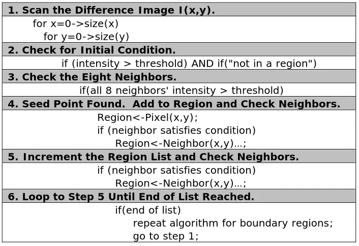
The following table shows the pseudo code for the region growing separation algorithm, resulting in distinct regions of inside points and boundary points.
Table 2: Pseudo Code for Inside Point / Boundary Point Region Growing
1. Scan the Difference Image I(x,y).
for x=0->size(x) for y=0->size(y)
2. Check for Initial Condition.
if (intensity > threshold) AND if("not in a region")
3. Check the Eight Neighbors.
if(all 8 neighbors' intensity > threshold)
4. Seed Point Found. Add to Region and Check Neighbors.
Region<-Pixel(x,y);
if (neighbor satisfies condition) Region<-Neighbor(x,y)…;
5. Increment the Region List and Check Neighbors.
if (neighbor satisfies condition) Region<-Neighbor(x,y)…;
6. Loop to Step 5 Until End of List Reached.
if(end of list)
repeat algorithm for boundary regions; go to step 1;
14
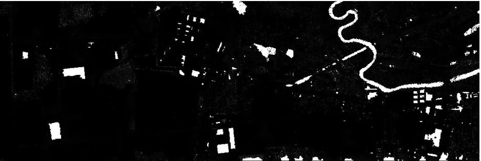
Figure 7: Inside Point Region Identification
In a direct comparison with Figure 3, Figure 7 illustrates the algorithms ability to identify non-ground pixels effectively. Moreover, it also illustrates the ability of the algorithm to identify regions of interest based upon a defined threshold that can be preset by the user. This allows for a height threshold specification for inclusion, allowing for the elimination of other non-ground objects that are not necessarily buildings, objects such as cars, shrubs, and other vegetation.
Figure 8 below shows the boundary point regions, once again identified by the shade of white in the image.
Figure 8: Boundary Point Region Identification
Plane-fitting techniques
The above algorithm successfully resolved the non-ground pixels into two distinct types,
boundary points and inside points. The region growing process allowed these two distinct types of pixels to be represented as grown region areas with clearly defined boundaries. However, in order to reduce inclusion errors present in any region growing process, further segmentation of the inside point regions is necessary. The process involved in this further segmentation employs the use of a plane-fitting technique to separate inside point regions into smaller regions
representing building surfaces. The overall goal is to segment each inside point region into smaller regions based on the formation of best-fit planes of pixels and their neighbors, resulting in a representation of planar surfaces within each inside point region.
The plane-fitting process used is a least-squares method of determining a best-fit plane from a given number of three-dimensional points. The algorithm determines a plane that best fits nine distinct three-dimensional points, in this case an inside point pixel and its eight neighboring pixels. The solution provides the least squares solution to the following equation:
C By Ax y x
I( , )= + + (3)
with I(x,y) representing the intensity of the pixel located at coordinate (x,y) and A,B,C
representing parameters of the best-fit plane determined from the nine pixels in question. The goal of this least squares solution is to minimize the sum of the squared errors between the pixel intensity values and the resulting intensity value when using the plane equation (3).
Given a set of pixels
{
[
xi,yi,Ii(
xi,yi)
]
}
9i=1 under consideration, a function is defined as follows:(
)
9[
(
) (
)
]
21 , , ,
∑
= − + + = i i i i ii By C I x y
Ax C
B A
E (4).
The function is defined in such a way that all values are positive and the vertex of the resulting hyperparabaloid occurs when the gradient satisfies the condition∇E=
(
0,0,0)
. This condition results in the following system of three simultaneous equations which can be solved for the best-fit plane of the given nine pixels:(
)
∑
[
(
) (
)
]
(
)
= − + + = = ∇ 9 1 1 , , , 2 0 , 0 , 0 i i i i i i ii By C I x y x y
Ax
E (5).
Equation (5) results in the following matrix equation:
(
)
(
)
(
)
⎥⎥ ⎥ ⎥ ⎦ ⎤ ⎢ ⎢ ⎢ ⎢ ⎣ ⎡ = ⎥ ⎥ ⎥ ⎦ ⎤ ⎢ ⎢ ⎢ ⎣ ⎡ ⎥ ⎥ ⎥ ⎥ ⎦ ⎤ ⎢ ⎢ ⎢ ⎢ ⎣ ⎡∑
∑
∑
∑
∑
∑
∑
∑
∑
∑
∑
∑
= = = = = = = = = = = = 9 1 9 1 9 1 9 1 9 1 9 1 9 1 9 1 2 9 1 9 1 9 1 9 1 2 , , ,1 i i i i
i i i i i i i i i i i
i i i i
i i i i
i i i
i i i i i
16
The above matrix equation is solved for the parameters A, B, and C respectively which defines the best-fit plane of the nine pixels in question. With these parameters determined, a plane-fitted intensity value can be found for any of the pixels in question. This plane-fitted intensity value can then be used in comparison with the actual intensity value observed at the pixel in question in order to create a condition for a region growing procedure that will allow segmentation into surface regions.
In order for this condition to be used in the region growing process, an initial seed point must be determined. Therefore, an additional detail is added to the region growing processes above – the calculation of the ABC parameters for each inside point pixel determined in the inside point segmentation process. Therefore, when a pixel meets all criteria for inclusion in an inside point region, a best-fit plane for the pixel and its eight neighbors is calculated. Along with these ABC parameters for the plane equation, the minimum sum of squared errors (SSE) is also calculated for each inside point according to the following equation:
(
)
[
]
2, i
i actual i
i By C I x y
Ax
SSE= + + − (7)
with xi and yi representing the coordinate of the pixel in question and Iactual(xi,yi) representing the actual intensity value at the pixel in question. This equation represents the sum of squared error calculation, determined by the square of the difference between the calculated best-fit intensity value and the actual pixel intensity value at the specific coordinate being analyzed.
This SSE calculation allows an initial seed point to be determined for the surface growing
algorithm. Once an inside point region is completely grown, all best-fit plane parameters and the corresponding SSE for any inside point and its eight neighbors has been determined using the matrix equation (6). The linked list that houses the inside point region pixels and this best-fit plane data is now sorted in ascending order according to the SSE, effectively determining the minimum SSE value for the inside point region in question. The inside point with the minimum SSE determined through the plane-fitting algorithm is added to the surface region. The reason for this minimum SSE being the condition for initial inclusion in the surface algorithm is that the inside point with the smallest SSE value has the most accurate best-fit plane associated with it and its eight neighbors. This allows a fairly accurate plane representation, and therefore the best chance for a smooth surface to be determined from pixels in a particular area, for example a face on a roof of a building. The goal is to grow surfaces in this particular algorithm, so the condition must allow for the best possible surfaces to be grown, which is accomplished by selecting the inside point with this minimum SSE value.
range and therefore is not a close enough fit to be included in the surface. However, if the calculated height difference is less than this Δh threshold, then the pixel is a close enough fit to the growing surface and is included in the surface region.
This testing continues until all eight neighbors have been tested for inclusion in this particular surface region. Once the eight neighbors have been completely checked, the pointer to the linked list containing the surface region values is incremented, and further testing is performed on the eight neighbors of this point. This process continues until the surface region has been fully traversed and no further growing can be performed, effectively ending the surface in question.
However, testing does not stop here. Every point within the inside point region must be added to a surface, and thus far, only the initial surface determined from the minimum SSE inside point has been accounted for. Therefore, the linked list pointer to the inside point region is
incremented, finding the second smallest SSE value. If this point does not already belong to a surface, then this inside point becomes the new initial seed point, and surface growing begins again in the same fashion. This process continues until the end of the inside point region is reached, completing the traversal of the entire inside point region.
The fact that every inside point must belong to a surface results in surfaces of various sizes. If, for instance, an inside point on the outer edge of an inside point region becomes the seed point, the SSE may be the largest without regard to the plane-fitting algorithm’s calculations on the “smoothness” of a group of pixels, and the surface grown would be extremely small because the surrounding pixels may not lie within the defined height threshold, possibly resulting in a surface of only one pixel if no other points fit the plane for that seed point. The process is rather
complicated in this sense but works as desired for breaking up the larger inside point regions into sub-regions with conditions that define well defined surfaces. This further segmentation results in many more surfaces than inside point regions, separated by their relative fit to the region in general.
For the test area in Lenoir County, North Carolina shown in figure 3, there were 218 inside point regions found and 1655 surfaces determined from these points. This much greater number of surfaces shows that the conditioning performed in this surface growing algorithm vigorously separate the inside point regions, resulting in a much finer conditioning and therefore datasets that share very similar properties which can be used to refine the building footprint algorithm drastically.
Merging of Building Surfaces
With the non-ground points now completely segmented into surfaces, the next step is simply an adjustment phase, hoping to help eliminate any errors that may have become prevalent in the previous steps. Because the segmentation above relies on thresholds in order to separate pixels and determine building footprints from these separated pixels, the quality of the building footprints and the amount of errors present in them are all determined by how closely the
18
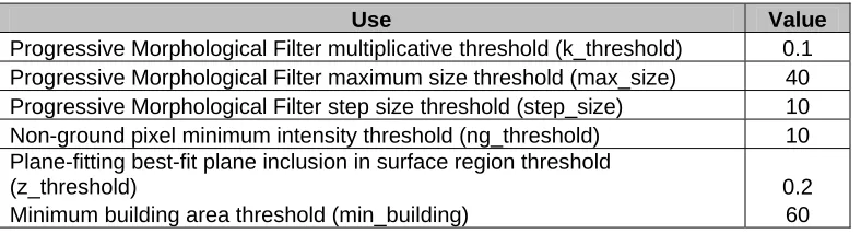
Table 3: Various Thresholds Used in Algorithms
Use Value
Progressive Morphological Filter multiplicative threshold (k_threshold) 0.1 Progressive Morphological Filter maximum size threshold (max_size) 40
Progressive Morphological Filter step size threshold (step_size) 10 Non-ground pixel minimum intensity threshold (ng_threshold) 10 Plane-fitting best-fit plane inclusion in surface region threshold
(z_threshold) 0.2
Minimum building area threshold (min_building) 60
All of the above threshold values have been explained in the sections above relative to their use in the algorithms they are associated with. However, there is another threshold mentioned here that has not been discussed yet, which relates to the merging of building surfaces which allows the final building footprints to be determined. In order to eliminate small patches of vegetation, a minimum building area must be determined. This minimum area threshold is set to 60 square meters, encompassing an area of three pixels on average, so any inside point regions having less than three pixels are neglected in the building separation process.
Building Footprint Post-Processing
The building footprints for the particular area of Lenoir County, North Carolina considered thus far have been determined using the region growing algorithm. Inside points and boundary points were identified, and the resulting images have been displayed. However, the building footprints that have been identified are noisy since LIDAR data is inherently irregularly spaced. Therefore, some simplification of these noisy footprints must be performed. In the boundary point figure above, the edges of identified buildings have a zigzag quality and need to be simplified into a line that represents the true building boundary. Many simplification algorithms exist, but the Douglas-Peucker algorithm was implemented to simplify the noisy building footprints.
The Douglas-Peucker Algorithm
One such technique to develop a cleaner building footprint is the Douglas-Peucker algorithm, an algorithm developed by cartographers D.H. Douglas and T.K. Peucker in [7]. The Douglas-Peucker algorithm allows for a simplification of any polyline by a recursive threshold technique.
The Douglas-Peucker algorithm operates on the boundary point regions identified by the conditioning described above. An initial simplification guess begins the process. For each boundary point region, the initial guess contains the first boundary pixel in the region and the last boundary pixel in the region connected together to form a line segment. The algorithm then determines whether the initial guess of a line segment is a good enough simplification for the polyline in question. This determination is performed based on a user-defined distance threshold.
Assuming the boundary point regions represent buildings, a line segment should never be a good enough simplification in this case. Therefore, further processing is necessary. The entire
line segment is calculated. If the boundary point in question is within the outer limits of the initial guess line segment, a perpendicular distance is calculated. If the boundary point in question is on either side of the outer limits of the initial guess line segment, then the distance from either the left endpoint of the initial guess (the boundary point is on the left side of the initial guess line segment) or the right endpoint of the initial guess (the boundary point is on the right side of the initial guess line segment) is calculated. This distance calculation is measured in pixel units, with each side of a pixel considered to have unit length.
Once all boundary point pixels in the region have had distances from the initial guess line segment calculated, the boundary point pixel at which the maximum distance from the initial guess line segment is identified. This maximum distance value is compared to the distance threshold provided by the user, and if the maximum distance is less than this threshold value, then the initial guess line segment was an accurate enough simplification, and the new boundary point region contains only two points, the endpoints of the initial guess line segment. However, if the maximum distance is greater than the threshold value, then the initial guess line segment was not accurate enough, and further processing must be performed.
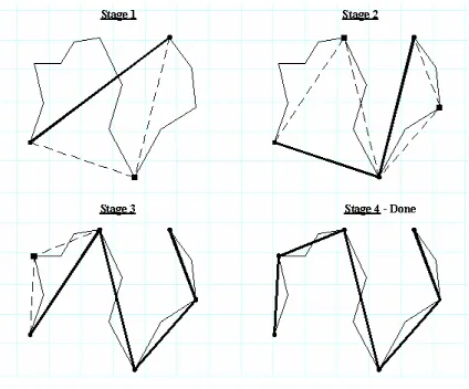
Assuming the initial guess line segment was not accurate enough, a new guess is determined. The pixel at which the distance threshold was exceeded becomes one of the endpoints of two new line segments representing the new guess. The first point of the boundary point region is connected to this maximum distance pixel to form a line segment, and this maximum distance pixel is connected to the last of the boundary point region to form another line segment. Each line segment is now assumed to be a new initial guess, and the process continues recursively until all boundary point calculated distances are less than the user-defined threshold. The figure below illustrates the process described above.
Figure 9: Visualizing the Douglas-Peucker Algorithm
20
distance results in one final user-defined threshold being exceeded, stage 4 results in the simplified polyline shown above.
The figure below shows the Douglas-Peucker algorithm result with a distance threshold value of 2.4.
Figure 10: Douglas-Peucker Algorithm Resulting Image
Chapter 4
Region Growing Algorithm Improvements
With the algorithms completed and the building footprints successfully extracted, ways to possibly improve results were considered. It was noted that the possible improvements could exist when the boundary point regions were initially identified. The resulting footprints were extremely noisy, and therefore simplification seemed to be a difficult process. Therefore, a new way of defining boundary points was considered, and a new method of growing the boundary point regions was developed.
Boundary Point Identification
Boundary points were initially identified as any pixel in the difference image which had a value greater than a height threshold that also had at least one neighboring pixel identified as a ground pixel. This definition is somewhat incomplete, considering that any boundary point should also have a neighboring pixel identified as an inside point. Therefore, the definition of what
constitutes a boundary point was made more strict, requiring the intensity of the difference image to be greater than the given height threshold, at least one neighboring pixel identified as a ground pixel, and at least one neighboring pixel identified as an inside point. It was believed that this extra condition would obviously result in fewer pixels to pass the boundary pixel test, and therefore result in less overall boundary pixels and a better overall simplification of the building footprints and a less noisy one as well. The figure below shows the identification of boundary footprints with this new definition.
Figure 11: Boundary Point Region Identification – New Definition
The above image with boundary pixels colored white shows a definite improvement in the reduction of noisy edges from the original boundary point figure identified in Chapter 3. A
22
Boundary Point Region Growing
While there is a noticeable improvement in the identification of boundary points via the new definition, the footprints are still noisy enough to require further processing improvements. The Douglas-Peucker algorithm result illustrated above was not an acceptable simplification in all cases. It was determined that the Douglas-Peucker algorithm is extremely order intensive, in the sense that the order that the boundary points were placed into regions was extremely important in the determining a successful resulting simplification.
Boundary points were initially sorted through by scanning the difference image from the left portion of the image to the right part of the image in a top-down manner. The entire difference image was scanned for each boundary point region, a fairly inefficient process. Also, because of the left-to-right, top-down identification of the boundary point regions, the order of the boundary points could become scattered and not representative of buildings. Initially, this did not seem to be causing a problem, but once the Douglas-Peucker algorithm was implemented on these unordered boundary point regions, the result was clear. Because the Douglas-Peucker algorithm only checks distances of points to the initial guess on points that exist between the endpoints of the initial guess, ordering is extremely important. The Douglas-Peucker algorithm approximates the polyline obtained by connecting every boundary point in the order that they are added to the region.
Therefore, the goal was set to develop a sorting algorithm that would order boundary points in a way that, if each boundary point in the region were connected to the adjacent boundary points in the region, the result would be exactly as shown in the boundary point region figure above, that is they would represent the buildings that are to be simplified. The sorting was performed by using a variation on the region growing algorithm. First, the definition condition of a boundary point must be satisfied. Once a pixel satisfied this condition, the pixel was labeled as a boundary point and added to the region.
The next step is key to the development of a successful sort. The region growing algorithm described above would check every neighbor and add any pixels that satisfied the condition to the region. However, this could in some cases add more than neighbor to the region if more than one neighbor satisfied the condition. This would cause a problem in the ordering, as it is desired for the sort to represent a point-to-point connection of the boundaries of buildings. If more than one neighbor were added to the boundary point region for satisfying the boundary condition, then the corners of buildings would not contain a point-to-point connection. Therefore, once a seed point for the boundary point region was determined, the region growing algorithm begins. However, if two or more neighbors satisfy the boundary condition, only the first point is added to the list, and the region growing process continues in whatever direction this point was from the seed point. All boundary points obtained via the new definition by the original left-to-right, top-down scan are contained in this new region growing scan.
Figure 12: Douglas-Peucker Algorithm – Improved Sort
The resulting image shows that the Douglas-Peucker algorithm with this modified sorting mechanism improves upon the previous top-down sorting run. A comparison of particular problem areas will be shown in the next chapter.
Satellite Image Processing
The resulting images above show that the algorithms for identifying building footprints
successfully identify buildings. However, it was desired that there be data available to use in the future for possible comparison purposes, that is the ability to compare the obtained LIDAR building footprints with some other form of data to determine how accurate the LIDAR building footprints were.
In [1] Zhang performs a visual comparison to aerial photos by overlaying the obtained footprints over the aerial image to determine how accurate the LIDAR building footprints were. Contrary to Zhang, this particular satellite comparison algorithm attempts to provide a tool to compare the obtained LIDAR footprints to satellite imagery automatically.
24
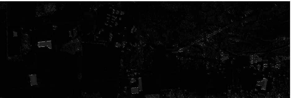
Figure 13: Satellite Image Data
The goal is to perform a region growing algorithm on the above satellite image. The condition to include a point in a particular region is the Euclidean distance between the associated RGB color intensities. This color region growing algorithm will provide regions that have similar color within a user-defined color threshold. The area of each region along with the average values of the x and y coordinates of the pixels in each region are calculated. The areas of the inside point and boundary point regions along with their average x and y coordinates were calculated with the region growing approach above. The claim is that with this data, buildings can be separated from vegetation based on color characteristics, which could prove helpful in removing false building identifications that could occur in dense forest areas. Also, if some areas and averages obtained from the inside/boundary region growing algorithm are similar to the areas and
averages obtained from this color region growing algorithm, this algorithm could provide confirmation that the LIDAR building footprints were obtained accurately without visual inspection.
Because all points must be grown into corresponding color regions, there is no initial condition for selection of a seed point. The seed point is selected on the condition that it has not already been placed in a region, and it is then added to a region, and its color is identified according to its red, green, and blue components. Then, a condition is placed on its eight neighbors according to the following equation:
2 2
2
) (
) (
)
( seed neighbor seed neighbor seed neighbor
color R R G G B B
D = − + − + − . (8)
26 Chapter 5
Comparative Results
In Chapter 4, the results of changing the original approach to the region growing algorithm were presented, and it was shown that there was visual confirmation of improvement in the
identification of building footprints. However, a side-by-side comparison will further show the effect the above changes have had on the building footprint results.
The figure below shows an enlarged section of the Lenoir County study area, comparing the old boundary point definition to the new boundary point definition.
Figure 14: Boundary Point Identification – Comparison
This building footprint comparison clearly shows that redefining what a boundary point really is results in a less noisy and simplified footprint that more accurately represents the actual building boundaries. The extreme jagged nature of the footprint on the left is replaced by a fairly smooth representation on the right, considering that LIDAR data is irregularly spaced and therefore noisy to begin with.
Yet another comparison figure below shows a problematic area in the original Douglas-Peucker algorithm and its improved result.
Figure 15: Douglas-Peucker Algorithm – Comparison
This simplification comparison shows the obvious improvement in building footprint
footprints. The figure below shows the connection of points for two buildings after Douglas-Peucker simplification, clearly showing the successful simplification.
Figure 16: Douglas-Peucker Algorithm – Example Simplification
Conclusions
The goal of extracting building footprints from a LIDAR dataset was completed successfully. Redefining what constitutes a building boundary point helped to improve the Douglas-Peucker algorithm’s identification of building corners and improved the simplification process. The additional ability to grow regions based on the RGB color attributes in a satellite image allows for confirmation or disconfirmation of building footprints. This ability to automatically prove or disprove the validity of the extraction of building footprints improves upon simple visual
inspection of aerial or satellite imagery for such purposes.
Future Work
Even though the algorithms above successfully identify building footprints and provide a means for comparison with satellite imagery, future work is available. Actual comparisons could be performed by sorting the color regions and inside/boundary regions according to areas and attempting to find similarities between them, confirming building locations and possibly removing dense forestry areas misidentified as buildings. Also, with building footprints
28 References
[1] K. Zhang, J. Yan, and S.-C. Chen, “Automatic Construction of Building Footprints From Airborne LIDAR Data,” IEEE Transactions on Geoscience and Remote Sensing, vol. 44, no. 9, pp. 2523-2533, Sept. 2006.
[2] K. Zhang, S.-C. Chen, D. Whitman, M.-L. Shyu, J. Yan, and C. Zhang, “A Progressive Morphological Filter for Removing Non-Ground Measurements from Airborne LIDAR Data,” IEEE Transactions on Geoscience and Remote Sensing, vol. 41, no. 4, pp. 872-882, Apr. 2003.
[3] Saleh, Bahaa E.A. and Malvin Carl Teich, Fundamentals of Photonics. Wiley Interscience, 1991.
[4] “LIDAR Accuracy: An Airborne 1 Perspective.”
http://www.airborne1.com/technology/LiDARAccuracy.pdf
[5] Gonzalez, Rafael C., Richard C. Woods, and Steven L. Eddins, Digital Image Processing Using MATLAB. Prentice Hall, 2003.
[6] http://seattlepi.nwsource.com/local/19144_quake18.shtml
[7] D. H. Douglas and T. K. Peucker. Algorithms for the reduction of the number of points required to represent a line or its caricature. The Canadian Cartographer, 1973.
[8] http://www.csc.noaa.gov/products/sccoasts/html/tutlid.htm
Vita
Henry Christopher George was born in Metairie, Louisiana. He is a graduate of the Jesuit High School class of 2001 with the distinction Summa Cum Laude. He received his Bachelor of Science in Electrical Engineering from the University of New Orleans in 2005 with the distinction of Magna Cum Laude.