Derivation of Shadow Price for CO2 Gas Emission
Using Distance Function Approach
Gholamali Sharzehi∗ Morteza Molaei∗∗
Abstract
The purpose of this study is to estimate the shadow price of CO2 gas emission utilizing the output distance function including good products (GDP) and bad products (CO2). At the first, output oriented technical efficiency under the two assumptions of weak and strong disposability of CO2 and Environmental Efficiency Index are estimated using the Iran’s economic data. Shadow price of CO2 gas emission is derived employing a Translog distance function.
Results show that the average of technical efficiency under the two assumptions of strong and weak disposability and environmental efficiency are equal to 1.0743, 1.0910 and 0.99267, respectively. Average shadow price of CO2 emission is 0.10933 million US dollars per thousand tons based on the constant price of the year 2000.
Keywords: Environmental Efficiency, Shadow Price of CO2, Distance Function, Iran.
∗ Associate Professor, Faculty of Economics, University of Tehran
∗∗ Ph.D. student, Agricultural Economics Department, University of Tehran
1- Introduction
Environmental problems are threatening world’s sustainability. At current rates of emission, the accumulation of greenhouse gases in the upper atmosphere is expected to elevate average global surface temperature by approximately 0.3–2.5°C in the next 50 years and 1.4–5.8° C in the next century (Zelek and Shively, 2003). Economic and ecological impacts of global warming are one of the most important debates.
Global climate problems led the international agreement at the Earth Summit in 1992 to reduce greenhouse gas emissions by 2000 to the level of 1990. Afterward, Kyoto Protocol in 1997 under which industrialized countries agreed to legally binding emissions reduction averaging about 5 percent of 1990 levels by period 2008-2012 (Kumar and Khanna, 2002). In Kyoto Protocol, no numerical targets for emissions of developing countries, like Iran, were set. But on one hand, the cost of air pollution is 1.6 percent of GDP and on the other hand, the cost of environmental degradation is about 10000 million US$ annually and close to 8.8 percent of Iran’s GDP (World Bank, 2005). Also environmental problems are not only matters of regional significance, but have taken on global significance. Therefore, studying the negative impacts of pollution emission on economic growth make sense for Iran.
To reduce these negative impacts, it is necessary to regulate pollution emission. Estimating marginal cost of abatement will help the country analyze the cost effectiveness of alternatives ways to reduce emission, predict environmental effects of economic growth, and make decision about trading international tradable pollution permit.
The most important greenhouse gas, and the one has received the most attention is Carbon Dioxide (Zelek and Shively, 2003; Zaim and Taskin, 2000; Tahara et al, 2005).
2- Methodology
2.1. The Technology SetSuppose a country is a decision making unit (DMU). This DMU employs a vector of inputs x(=x1, x2,…, xK) to produce a vector of desirable
output y (=y1, y2, …, yM) and a vector of undesirable outputs b (=b1, b2,
…,bN), where K, M and N are non-negative. Let P(x) be the production
possibility set for a given input vector x and L(y , b) is the input requirement set for a given level of output (y , b). The technology set is defined as (Fare and Grosskopf, 2000):
T=
{
(y,b,x)∈RM+N+K,(y,b)∈P(x),x∈L(y,b)}
(1)Now, suppose the desirable (good) and undesirable (bad) outputs are null-joint; that is, the production of good outputs are accompanying with bad outputs production, thus if (y,b)∈P(x) and y=0 then b=0.
There are two assumptions about the disposability characteristic of bad outputs that if they are strongly (freely) to dispose or weakly dispose. Strong disposability means that the disposition of bad outputs is not costly (Fare et al, 1993).
If
) ( ) , ( ) , ( ) , ( ) ( ) ,
(y b ∈P x and y′b′ ≤ y b ⇒ y′b′ ∈P x (2)
Equation (2) implies that if an output set is feasible with a given level of inputs then every other output set smaller than it is feasible with the same level of inputs. But weak disposability of bad outputs says that the DMU have to divert the resources from good production to dispose of bad outputs, so the disposition of bad outputs is costly (Fare et al, 1993).
If
) ( ) , ( 1 0
) ( ) ,
(y b ∈P x and ≤
θ
≤ ⇒θ
yθ
b ∈P x (3)inputs, the constant returns to scale (CRS) output set P(xC,S) can be constructed by means of
P(xC,S)
= ⎭ ⎬ ⎫ ⎩ ⎨ ⎧ ∈ ≤ ≥ ≥ + = = =
∑
∑
∑
T T t t tN t T t t tM t T t t tMty y z b b z x x z R
z b y 1 1 1 , , , : ) ,
( (4)
Where C and S referee to constant returns to scale and strong disposability of bad output, respectively and z (=z1, z2… zT) is the vector of
intensity variable (Zaim and Taskin, 2000). Similarly, a CRS technology satisfying the weak disposability of undesirable outputs and strong disposability of desirable outputs and inputs can be represented as an output set as shown below (Zaim and Taskin, 2000):
P(xC,W)
=
⎭
⎬
⎫
⎩
⎨
⎧
≥
=
≤
∈
+ = = =∑
∑
∑
T Tt t tN t T t t tM t T t t tM
t
y
y
z
b
b
z
x
x
z
R
z
b
y
1 1 1,
,
,
:
)
,
(
(5)where W referees to weak disposability of bad output.
Equations (4) and (5) construct a best practice technology from the observed data on inputs and outputs relative to which technical efficiency of the production of each year can be calculated.
There are two alternatives of technical efficiency: input oriented and output oriented measures of technical efficiencies and there are two approaches to measure it: parametric and nonparametric. Stochastic Frontier Analysis (SFA) is used to estimate technical efficiency in parametric approach and Data Envelopment Analysis (DEA) in nonparametric. In this paper, we want to calculate the output oriented measure of technical efficiency using DEA that can be shown as below (Fare and Grosskopf, 2000):
{
: ( , ) ( )}
max ) , ,(y b x y b P x
Where
θ
is efficiency index. The reciprocal of this index shows the output distance from production frontier, and defined as (Kumar and Khanna, 2002):⎭
⎬
⎫
⎩
⎨
⎧
∈
=
min
:
(
(
,
)
)
(
)
)
,
,
(
y
b
x
y
b
P
x
D
θ
θ
(7)The distance function, defined by Shepherd (1970), equal to one shows that the DMU operates at the production frontier and when the DMU operates below the frontier, distance function is smaller than one but greater equal than zero. The output distance function has three advantages (Fare et. al, 1993): first, it allows to model bad outputs; second, it can describe completely the technology and models joint production of multiple outputs; third, the duality between distance and revenue function allows generating shadow prices of outputs. The output distance function measures the maximum proportion by which all outputs increased proportionally when the inputs are held constant but reduction in bad outputs will divert inputs to good outputs. Therefore, the output distance function should be non-decreasing in good outputs and non-increasing in bad outputs and inputs.
2-2- Environmental Efficiency
The output distance function can be used to estimate the environmental efficiency (EE) with respect to bad output. From Zaim and Taskin (2000) EE is the ratio of the square root of the output distance function under strong disposability of bad output to the square root of the output distance function under weak disposability of bad output (Kumar and Khanna, 2002).
EE=
)
,
,
,
(
)
,
,
,
(
W
C
x
b
y
D
S
C
x
b
y
D
t t t
t t t
(8)
2-3- Shadow Price of Bad Output
Pittman (1983) employed a profit function to estimate the shadow price of bad outputs. But Fare et al (1993) introduced an alternative way. They showed how the output distance function can be used to generate shadow prices of bad outputs. They estimated an output distance function and employed a dual Shepherd’s lemma to calculate shadow price of outputs both for marketable and no marketable outputs. As noted by Fare et al (1993) “the ratio of any two of these output shadow prices reflects the relative opportunity cost of those outputs, i.e., they are equivalent to the marginal rate of transformation”. The shadow price of bad output calculated by means of this method reflects the marginal cost of abatement and the trade-off between bad and good outputs. The shadow prices of bad (rb)
outputs can be calculated as follows (Fare et al, 1993):
y W C x b y D
b W C x b y D r r
t t t
t t t
y b
∂ ∂
∂ ∂
× =
) , , , (
) , , , (
(9)
where ry is the price of good output.
2-4- Estimation Method and Data
T x T b T y T T x b x y b b b y y y x x x W C x b y D t k M k kt t n M n nt t m M m mt tt t t k t n K k N n kn t k t m K k M m km t n t n N n N n n n t n N n n t m t m M m M m m m t m M m m K k t k t k K k K k k k t k k t t t t × + × + × + × + × + + + + + + + + + =
∑
∑
∑
∑∑
∑∑
∑∑
∑
∑∑
∑
∑
∑∑
= = = = = = = ′ = ′= ′ = ′ = ′= ′ = = ′ = ′ ′ ln ln ln 2 1 ln ln ln ln ln ln 2 1 ln ln ln 2 1 ln ln ln 2 1 ln ) , , , ( ln 1 1 1 2 1 1 1 1 1 1 1 1 1 1 1 1 0 θ θ θ θ θ ϕ δ λ γ β β α α α (10)To estimate the functional form (10), it must be imposed the restrictions on symmetry and homogeneity. Equation (11) and (12) below show the homogeneity degree 1 of output distance function in outputs and the symmetry condition, respectively.
1
1 1=
+
∑
∑
= = N n n M m mγ
β
(11)n n n n m m m m k k k k kn km n n m m k k ′ ′ ′ ′ ′ ′ ′ ′ ′ = = = = = = = =
∑
∑
∑
∑
∑
γ
γ
β
β
α
α
ϕ
δ
γ
β
α
0 (12)The parameters of functional form (10) estimated using the parametric approach.
3- Results
3-1- The output distance function
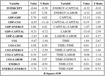
In table 1, estimated parameters for the output distance function under weak disposability of CO2 are presented. The first derivative of the model with respect to all input variables (except for capital), time variable and undesirable output (CO2 emission) have negative signs but have positive sign with respect to GDP. The negative signs on inputs indicate that output distance function value is non-increasing with respect to inputs and economy becomes closer to the frontier.
Coefficients of the time variables indicate the presence of technological progress in the regression model. A negative sign for all of time variables shows technological progress but positive sign for that shows technological deterioration. In this study, except for time variable and interaction term between capital and time, all time variables have negative signs. On the other hand, negative sign of first order derivative of distance function with respect to time shows technological progress.
Table 1: Parameter Estimates of Output Distance Function
3-2-Environmental Efficiency
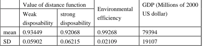
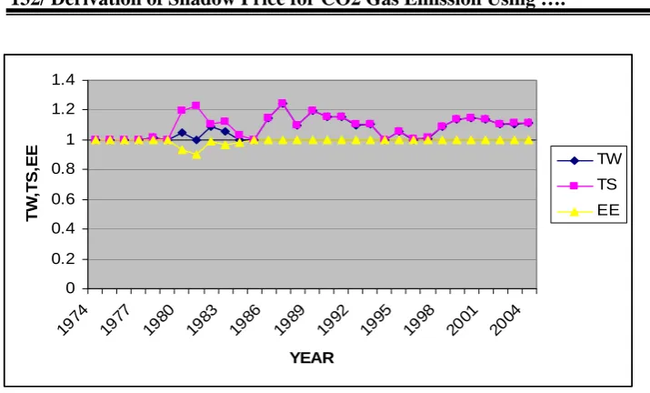
An increase in GDP along with CO2 reduction means efficiency gain in environmental terms. Recall that the output distance function can be used to calculate environmental efficiency. If the values of distance function under two assumption of weak and strong disposability of CO2 are the same then EE equal to one and CO2 emission can be abated without reducing GDP; but if they are different, country has an environmentally binding production technology. Figure 1 shows trends for the value of technical efficiency under two assumptions of weak and strong disposability of CO2. The figure also shows environmental efficiency of Iran economy for period 1974-2004. Table 2 presents mean values for output distance function under weak and strong disposability and environmental efficiency, too. Except for most years of the study, environmental efficiency is less than one (figure 1) and also average environmental efficiency is less than one (table 2) that reflects Iran has an environmentally binding production technology. The absolute GDP loss due to weak disposability of CO2 can be calculated as GDP×(1-EE). Therefore, on average, GDP loss is equal to 1158 millions of 2000 US dollar to use the best practice technology.
Table 2: Mean Output Distance Function and Environmental Efficiency
Value of distance function
Weak disposability
strong disposability
Environmental efficiency
GDP (Millions of 2000 US dollar)
mean 0.93449 0.92068 0.99268 79394
SD 0.05902 0.06215 0.02109 19107
0 0.2 0.4 0.6 0.8 1 1.2 1.4
1974 1977 1980 1983 1986 1989 1992 1995 1998 2001 2004
YEAR
T
W
,T
S,
EE TW
TS
EE
Figure (1): Trends for Technical Efficiency under two assumptions of Weak and Strong Disposability of CO2 and Environmental Efficiency
TW= Technical Efficiency under Weak Disposability of CO2
SD= Technical Efficiency under Strong Disposability
EE= Environmental Efficiency
3-3-Shadow Price of CO2
Our results show that the average shadow price for decreasing of CO2 emission is $ 0.10933 millions per thousands metric tons ($109.33 per ton of CO2) at 2000 price.
Recall the estimation of shadow price of CO2 is suitable for decision making about predicting environmental effects of economic growth and trading international tradable pollution permits.
3-3-1- Predicting Environmental Effects of Economic Growth
As noted in section 2.3, shadow price of CO2 can be interpreted as marginal cost of abatement CO2 with respect to GDP and that shows a short term changes in environmental quality if GDP changes while technical efficiency remains constant.
environmental effects of economic growth, suppose as an example, Iran experiences GDP growth of %1 or US$ 1270.7515 millions, while efficiency remains constant. Shadow price, tells us that such increase in GDP results 11623.08 (=127075.15/0.10933) thousands tons or 2.95% increase in CO2 emission compared to the original value.
3.3.2. International Tradable Pollution Permit Trade
Since, first, Iran is not one of the members of Kyoto Protocol, and doesn’t have to reduce CO2 emission; second, trading international pollution permits is only possible for countries that have agreed to quotas, predominately the OECD countries; third, this study is not cross-country analysis; therefore, trading pollution permits is not applicable to this study. But we present an example to explain how Iran can use shadow price of CO2 for trading pollution permits.
Imagine a simplified version of Kyoto Protocol: two countries, Iran and an industrialized country such as Japan, enter an agreement to hold their total CO2 emission level constant. At this, suppose each country needs to emit more than what they do today. It should negotiate on the price with the partner and purchase a permit to emit additional pollution, while the other country should shrink its pollution by the amount sold.
4- Conclusions
The main purpose of this paper is to estimate shadow price of CO2 emission in Iran. Using time series data on Iran’s economy for the period of 1974-2004, technical efficiency under weak and strong disposability of CO2 are estimated by DEA (Data Envelopment Analysis) approach. Then output distance function that incorporates both desirable (GDP) and undesirable (CO2) outputs is estimated. The estimation of distance function is used to generate environmental efficiency index. But distance function estimation under weak disposability of CO2 is only used to derive shadow price of CO2.
Results show that Environmental efficiency (EE) and technical efficiency under the two assumptions are equal to one for most years reflects that Iran’s production technology satisfies strong disposability of CO2. It means Iran’s economy lies on production frontier; but for years that economy is away from production frontier, country has promising long-term perspective in simultaneous increase of GDP and decrease of CO2, should Iran improves the technology in use.
Our first illustrative example, based on the estimation of the shadow prices, showed how our estimates can be used in forecasting environmental outcomes of economic growth within a short run. Also, estimates of the efficiency allow us to conclude about technological feasibility and scale of potential simultaneous increase of GDP and decrease of environmental pollution.
References
1-Coelli, T. J., Battese G. (1996) Identification of Factors Which Influence The Technical Inefficiency of Indian Farmers, Australian Journal of Agricultural Economics, 40, 28- 103.
2-Coggins, J. S., Swinton J. R. (1996) The Price of Pollution: A Dual Approach to Valuing SO2 Allowances, Journal of Environmental Economics and Management, 30, 58-72.
4-Fare, R., Grosskopf S. (2000) Theory and Application of Directional Distance Functions, Journal of Productivity Analysis, 13, 93-103.
5-Fare, R., Grosskopf S. (2000) Reference Guide to On Front (The Professional Tool for Efficiency and Productivity Measurement,
www.emq.com
6-Fuentes, H. J. , Grifell-Tatje E. , Perelman S. (2001) A Parametric Distance Function Approach for Mulmquist Productivity Index Estimation, Journal of Productivity Analysis, 15(2), 79-94.
7-Kumar, S., Khanna M. (2002) The Impact of CO2 Abatement on Productivity Growth and GDP: A Cross Country Analysis Using the
Distance Function Approach,
www.ace.uiuc.edu/pERE/papers/pERE_WP29.pdf.
8-Murty, M.N., Kumar S. , Paul M. (2006) Environmental regulation, productive efficiency and cost of pollution abatement: a case study of the sugar industry in India, Journal of Environmental Management, 79, 1–9.
9-Pittman, Russell W. (1983) Multilateral Productivity Comparisons with Undesirable Outputs, Economic Journal, 93, 883-891.
10- Shepherd, Ronald W. (1970). Theory of Cost and Production Functions. Princeton University Press.
11- Tahara, K., Sagisaka M., Ozawa T., Yamaguchi K., Inaba A. (2005) Comparison of ‘‘CO2 efficiency’’ between company and industry, Journal of Cleaner Production, 13, 1301-1308.
12- World Bank, (2005) Cost of Environmental Degradation in Iran, Washington, DC.
13- Zaim, O., Taskin F. (2000) Kuznets Curve in Environmental Efficiency: An Application on OECD Countries, Environmental Efficiency and Resource Economics, 17, 21-36.