DEMOGRAPHIC RESEARCH
VOLUME 29, ARTICLE 43, PAGES 1187-1226
PUBLISHED 10 DECEMBER 2013
http://www.demographic-research.org/Volumes/Vol29/43/ DOI: 10.4054/DemRes.2013.29.43
Research Material
Integrating uncertainty in time series
population forecasts: An illustration using a
simple projection model
Guy J. Abel
Jakub Bijak
Jonathan J. Forster
James Raymer
Peter W.F. Smith
Jackie S.T. Wong
c
2013 Abel, Bijak, Forster, Raymer, Smith & Wong.
2 Data 1189
3 Statistical background 1191
3.1 Autoregression model 1191
3.2 Stochastic volatility model 1192
3.3 Random variance shift model 1192
3.4 Bayesian inference 1193
3.5 Model uncertainty 1194
4 Computation and forecasts 1195
4.1 Individual autoregressive models 1196
4.2 Individual stochastic volatility models 1202
4.3 Individual random variance shift models 1206
4.4 Model-averaged forecasts 1210
5 In-sample forecast validation 1213
6 Conclusion 1215
7 Acknowledgements 1216
References 1217
Integrating uncertainty in time series population forecasts:
An illustration using a simple projection model
Guy J. Abel1
Jakub Bijak2
Jonathan J. Forster2 James Raymer3
Peter W.F. Smith2 Jackie S.T. Wong4
Abstract
BACKGROUND
Population forecasts are widely used for public policy purposes. Methods to quantify the uncertainty in forecasts tend to ignore model uncertainty and to be based on a single model.
OBJECTIVE
In this paper, we use Bayesian time series models to obtain future population estimates with associated measures of uncertainty. The models are compared based on Bayesian posterior model probabilities, which are then used to provide model-averaged forecasts.
METHODS
The focus is on a simple projection model with the historical data representing population change in England and Wales from 1841 to 2007. Bayesian forecasts to the year 2032 are obtained based on a range of models, including autoregression models, stochastic volatility models and random variance shift models. The computational steps to fit each of these models using the OpenBUGS software via R are illustrated.
RESULTS
We show that the Bayesian approach is adept in capturing multiple sources of uncertainty
1Corresponding author: Wittgenstein Centre (IIASA, VID/ÖAW, WU), Vienna Institute of
Demogra-phy/Austrian Academy of Sciences, Austria. E-mail: [email protected].
in population projections, including model uncertainty. The inclusion of non-constant variance improves the fit of the models and provides more realistic predictive uncertainty levels. The forecasting methodology is assessed through fitting the models to various truncated data series.
1.
Introduction
In this paper, a detailed exposition of the Bayesian approach to time series forecasts of population totals is provided. The aim is to encourage the use of Bayesian methods by researchers interested in population forecasting. The main motivation behind this work is the need to incorporate the assessment of uncertainty into population forecasts (Alho and Spencer 1985; Keyfitz 1991; Lee 1998). The rationale for considering the Bayesian approach is that it offers a more natural framework than traditional frequentist methods to forecast future population with uncertainty. First, variability in the data and uncertainties in the parameters and model choice are explicitly included using probability distributions. Second, the predictive distributions follow directly from the probabilistic model applied. Third, it allows the incorporation of expert judgements, including their uncertainty, into the model framework. As a result, probabilistic population forecasts, with more reliable and coherent estimates of predictive uncertainty, can be obtained for a particular projec-tion model.
2.
Data
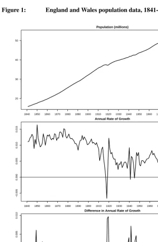
A historical series of the England and Wales population totals are used to introduce the Bayesian approach to time series forecasting. These data were obtained from The Hu-man Mortality Database4. The mid-year population totals from 1841 to 2007, including military personnel, are presented in the top panel of Figure 1. Here, we see that the popu-lation totals in England and Wales exhibited a steady increase over time, rising from 15.8 million in 1841 to 53.9 million in 2007. Brief periods of slight population decline are visible during the First World War and the 1918 influenza pandemic. Also noticeable is a period of levelling off in the population totals during the 1970s and 1980s, a result of net emigration and a lower rate of natural increase.
The features of population change are more evident when the annual rates of growth, plotted in the second panel of Figure 1, are considered. Detailed explanations for these patterns can be found in various books on British population history (Wrigley and Schofield 1989; Coleman and Salt 1992; Anderson 1996; Hinde 2003). The following provides a very brief account. The population growth rates were highest during the 1840–1910 pe-riod. This was predominantly due to the decrease in mortality occurring before the decline in fertility, which remained at pre-industrial levels for much of this period. Between the two World Wars, the rate of growth remained low in comparison with the later half of the 19th century and early 20th century. This was driven by the effects of low fertility from economic depression and a change in sociological factors. After the Second World War, population growth rates increased initially, through a short-lived fertility rise associated with demobilization, followed by a more substantial increase (baby boom) in fertility dur-ing the 1950s and early 1960s. In the late 1970s and early 1980s, the levels of population growth slowed down before rising in more recent decades though net immigration and higher fertility levels.
A time series of historical data is used to forecast the future rates of population growth. We are primarily interested in identifying the time series models that best fit these data in order ultimately to specify probabilistic intervals in forecasted populations. As we can see from Figure 1, the annual rates of growth have varied considerably over time. The models, described in the next section, provide alternative probabilistic specifications for this variation, and hence can be used to predict future variations in population change. These models are sufficiently flexible to describe a long series, and provide realistic pro-jections, without the need to choose a strategic starting point for the data series to best reflect future variation.
Figure 1: England and Wales population data, 1841-2007
Population (millions)
Time
1840 1850 1860 1870 1880 1890 1900 1910 1920 1930 1940 1950 1960 1970 1980 1990 2000 2010 20
30 40 50
Annual Rate of Growth
Time
1840 1850 1860 1870 1880 1890 1900 1910 1920 1930 1940 1950 1960 1970 1980 1990 2000 2010
−0.005
0.000
0.005
0.010
0.015
Difference in Annual Rate of Growth
1840 1850 1860 1870 1880 1890 1900 1910 1920 1930 1940 1950 1960 1970 1980 1990 2000 2010
−0.010
−0.005
0.000
0.005
3.
Statistical background
In this section, the models and notation used to forecast future annual growth rates in England and Wales are specified. The subsections introduce the autoregression models, stochastic volatility, random variance shifts, Bayesian inference and model uncertainty used in this paper.
Letptbe the population size at timet for an uninterrupted series of observed time
points. In population forecasting, we are interested in obtaining estimates ofptand the
associated measures of uncertainty for one or more values oft > T, whereT is the last observed time point.
In order to model pt, we first derive the time series of population growth ratesrt,
where
pt+1=pt(1 +rt). (1)
Note, we focus on the geometric growth rate to be consistent with the measurement of the population data, which have been measured in annual increments. A time series plot ofrtis presented in the second panel of Figure 1. It is clear that neither the mean nor
the variance of this series are stationary. Therefore, as advocated by Chatfield (2003), we consider the changes inrt:
yt=rt−rt−1. (2)
A time series plot ofytfor our data is presented in the third panel of Figure 1. It
ap-pears that an assumption of a stationary mean forytis appropriate. The assumption of
a stationary variance, however, is not justifiable. Hence, we need models to account for non-constant conditional variances, as presented in Section 3.2 and 3.3 below.
3.1 Autoregression model
There are several examples in the literature of autoregression (AR) models being used to forecast populations; see for example, Saboia (1974), Ahlburg (1987), Pflaumer (1992), Alho and Spencer (2005) and Tayman, Smith, and Lin (2007). An AR model of orderp, denoted AR(p), is defined as
yt= p X
j=1
φjyt−j+zt, (3)
whereφj are the autoregressive coefficients representing the correlations between
observations from a probability distribution with zero mean and constant variance,σ2. For
a fully-specified probability model, a normal distribution forztis typically assumed.
3.2 Stochastic volatility model
Stochastic volatility (SV) models have been widely used for modelling financial data, where the assumption of constant variance forztis usually untenable. Models that
ac-count for non-constant variance have been sparsely used in the demographic context (Keil-man and Pham 2004; Bijak 2010). This is surprising as historical time series of demo-graphic data often exhibit volatility due to events such as epidemics, wars or baby booms. This is certainly true for the data presented in Figure 1.
SV models are time series models, similar to the AR models defined in (3), but where the variance ofztis allowed to be time-dependent. This is achieved by replacingσ2with σ2
t, and specifying a time series model forσt2. In this paper, we assume an AR(1) model
forlogσ2
t. Here, let
σt2=eht (4)
and
ht=ψ0+ψ1(ht−1−ψ0) +η, (5)
wherehtrepresents the volatility at timet conditional on its own past,ψ0 denotes the
mean level ofhtover the entire time period whilstψ1is the autoregressive coefficient
rep-resenting the correlations betweenhtandht−1. Finally,ηare the error terms ofhtwhich
are assumed to be independent observations from a normal distribution with zero mean and constant varianceτ2. Other approaches to deal with non-constant variances include,
for example, autoregressive conditional heteroscedastic models (ARCH) and generalised ARCH models (GARCH); see for example Chatfield (2003). All of these approaches assume that the variance changes at each time step. An alternative approach, which we consider next, is to adopt a model where the variance changes at less frequent intervals, with intervening periods of constant variance.
3.3 Random variance shift model
ran-domly distributed factor, which we denote byeβt, so
σt=
σt−1 ifδt= 0 eβtσ
t−1 ifδt= 1
(6)
whereδtis a binary variable taking the value 1 if a variance shift occurs at time tand
0 otherwise. We model the sequence ofδtas independent Bernoulli random variables
withP(δt= 1) =, whereis the probability of the shift. The magnitude of a variance
shift, when it occurs, depends on the variableβtwhich is assumed to follow a normal
distribution with mean 0, and standard deviationλrepresenting the magnitude (on the log scale) of average variance shifts. The key feature of this model is that it adapts to periods of high or low volatility; thus forecasts of uncertainty during a period of low volatility will be predominately based on a lower variance than the overall level.
3.4 Bayesian inference
In Bayesian inference, uncertainty about the (multivariate) parameter θ of a statistical model is described by its posterior probability distribution given observed datay{T} =
{y1, . . . , yT}. The probability density function ofytis obtained by using Bayes Theorem:
f(θ|y{T}) =
f(y{T}|θ)f(θ)
f(y{T})
, (7)
wheref(y{T}|θ)is the likelihood function and is defined by the model,f(θ)is the prior distribution for θ and f(y{T})is a normalising constant. The prior distribution f(θ) specifies the uncertainty aboutθprior to observing any data.
Forecasting or prediction is particularly natural in a Bayesian framework. Uncertainty about the nextKfuture values ofyt(fort=T+ 1, . . . , T+K) is described by the joint
predictive probability distribution
f(yT+1, . . . , yT+K|y{T}) =
Z
f(θ|y{T})
K Y
k=1
f(yT+k|y{T+k−1}, θ)dθ. (8)
Note that the product term represents the joint predictive distribution in the case that parameterθis known. The Bayesian predictive distribution simply averages (integrates) this with respect to the posterior probability distribution forθ. Hence, uncertainty about
θin light of the observed data is fully incorporated.
the posterior distribution in (7) or the predictive distribution in (8). Performing these integrations analytically is often not possible for complex models, such as those described above. Historically, this has prevented demographers and others from taking advantages of Bayesian methods for statistical inference. More recently, this has become less of an obstacle as developments in Bayesian computation have improved. In particular, Markov chain Monte Carlo (MCMC) methods for generating samples from distributions, such as (7) or (8), have made it possible to apply Bayesian techniques to a wide variety of applications. Once a sample has been obtained from a joint distribution, then a sample from a distribution of any component or function of components is readily available; see Gelman et al. (2003) for details. To generate the samples from the posterior and predictive distributions for our study, we used the MCMC sampling approach implemented in the OpenBUGS software (Lunn et al. 2009). For each model, the performance of the MCMC sampler was assessed by standard visual inspection of time series traces of key parameters. After discarding any iterations required as burn-in, posterior summaries and projections were based on an MCMC sample of size of10,000. Details on the code to formulate the Bayesian time series models for OpenBUGS used in this paper are provided in the next section.
3.5 Model uncertainty
It is unrealistic for the analyst to be sure that any particular statistical model is the cor-rect one upon which to base their forecasts. Hence, the statistical methodology adopted should be one which allows for model uncertainty. Furthermore, we consider it essential that the measures of uncertainty associated with any forecast should incorporate both the uncertainty concerning the model and the uncertainty concerning the parameters of each model. Measurement error uncertainty inrtis practically insignificant relative to the size
of the population. In this paper, model uncertainty is directly integrated with parameter uncertainty into a single predictive probability distribution. A comprehensive review of Bayesian model averaging is available in Hoeting et al. (1999), and for some demographic applications, see Bijak (2010) and Bijak and Wi´sniowski (2010).
Formally, letm= 1, . . . , Mindex the models under consideration and letθm
repre-sent the parameter associated with modelm. Note that different models may have param-eters of different dimensionality. For example, the AR(2) model has a three-dimensional parameter (φ1, φ2, σ2). The likelihood function for modelmisf(y{T}|θm, m), the prior
distribution forθmisf(θm|m)and the posterior distribution is
f(θm|y{T}, m) =
f(y{T}|θm, m)f(θm|m)
f(y{T}|m)
wheref(y{T}|m)is a normalising constant, known as the marginal likelihood for model
m, and is given by
f(y{T}|m) =
Z
f(θm|m)f(y{T}|θm, m)dθm. (10)
Prior uncertainty about models is encapsulated by a discrete probability distribution,
f(m),m = 1, . . . , M. As we have no prior reason to prefer any model over any other, we give every model the same prior probability,1/M.
The posterior probability distribution formgiven observed datay{T} is obtained by using Bayes Theorem:
f(m|y{T}) =
f(y{T}|m)f(m)
f(y{T})
. (11)
Hence, the posterior model probability for any modelmis proportional to the product of the prior model probability and the marginal likelihood. Therefore, an efficient method for computation of marginal likelihoods is essential for Bayesian inference under model uncertainty (see, for example, those described in O’Hagan and Forster 2004). In our implementation, we found that the bridge sampler (Meng and Wong 1996) was effective for this computation.
Finally, to obtain a predictive distribution for population forecasts in the presence of model uncertainty, (8) is extended to
f(yT+1, . . . , yT+K|y{T}) =
M X
m=1
f(m|y{T})f(yT+1, . . . , yT+K|y{T}, m)
= M X
m=1
f(m|y{T})
Z
f(θm|y{T}, m)
K Y
k=1
f(yT+k|y{T+k−1}, θm, m)dθm (12)
which is the average of predictive distributions for individual models weighted by their posterior probabilities,f(m|y{T}).
4.
Computation and forecasts
models are provided in order to gain a better understanding of the effect of increasing the complexity of the model on future population growth rates. These individual forecasts are compared in Section 4.4 with a single forecast that incorporates uncertainty in model choice.
4.1 Individual autoregressive models
An initial set of nine models was considered for the differenced population growth rate,
yt, introduced in (1) and presented in the bottom panel of Figure 1. These consist of an
independent normal (IN) model and eight autoregression models, increasing in order from AR(1) to AR(8). This range of models was selected in order to represent all possible au-toregressive processes that might adequately describe the differences in the overall growth rate series. As we have no previous knowledge about the nature of the parameters in each model we assigned weakly informative prior distributions: φj ∼ N(0,1), j = 1, . . . , p
andσ−2∼Gamma(10−6,10−6), whereN(µ, σ2)denotes a normal (Gaussian) distribu-tion with meanµand varianceσ2, and Gamma(a, b)denotes a gamma distribution with shape parameteraand scale parameterb. As we also have no prior belief that the data should conform to a stationary regime, our prior distribution on the autoregression (φj)
parameters does not constrain the model to be stationary.
The computation of AR models were undertaken in OpenBUGS, where BUGS mod-els were produced using thear.bugsfunction intsbugsR package (Abel 2013). For example, a BUGS model for an AR(2) process on the difference of the population growth rate was created in R using the following code:
> library("tsbugs")
> r <- ts(ew[2:167]/ew[1:166]-1, start=1841) > y <- diff(r)
> ar2.bug <- ar.bugs(y, ar.order=2, k=25, beg=9)
print.tsbugscommand in R:
> print(ar2.bug) model{
#likelihood for(t in 9:190){
y[t] ~ dnorm(y.mean[t], isigma2) }
for(t in 9:190){
y.mean[t] <- phi1*y[t-1] + phi2*y[t-2] }
#priors
phi1 ~ dnorm(0,1) phi2 ~ dnorm(0,1)
isigma2 ~ dgamma(0.000001,0.000001) sigma <- pow(isigma2,-0.5)
#forecast
for(t in 166:190){ y.new[t] <- y[t] }
}
In the first part of the BUGS code, the likelihood for the AR(2) model is given. The random variabley[t], defined in the firstforloop is specified to come from normal distribution with mean y.mean[t] (defined in the second for loop) and precision
isigma2. The likelihood is based on data points y[9]to y[190], where the last
25 observations are treated as missing by BUGS and simulated values given the parame-ters estimates are generated. In the second part of the BUGS code, the prior distributions are given, which by default are created with the distributions stated at the beginning of this subsection. In the third part of the BUGS code, forecasted values ofytthat are
esti-mated in the likelihood part of the model, are duplicated and relabelledy.newto enable an easier handling of the BUGS output.
Thear2.bugobject in R has two additional elements, aside from the$bugs ele-ment, that are not printed. First, the$infoelement provides additional information on the data and BUGS model for use in other functions. The second is a cleaned version of the data formatted for use in R2OpenBUGS (discussed below). This is stored in the
$dataelement which can be displayed in R:
$y
[1] 1.598748e-04 9.949415e-04 3.466781e-04 8.274713e-04 -6.824515e-04 [6] -3.774363e-03 2.865602e-03 -1.522894e-03 6.070610e-03 -4.213722e-03 ...
[161] 3.303926e-05 4.433711e-04 1.470939e-03 3.009411e-04 -8.359634e-05
[166] NA NA NA NA NA
...
[181] NA NA NA NA NA
[186] NA NA NA NA NA
Note, the output above is edited to reduce space. The$datais a list namedy, to corre-spond to the 165 observed data points appended with 25 further missing data points to be forecast by the BUGS models.
Creating the BUGS model in R has two prominent advantages. Firstly, users can eas-ily run the estimation in OpenBUGS using the R2OpenBUGS package (Sturtz, Ligges, and Gelman 2005). Secondly, numerous output analysis and diagnostics for the MCMC simulations are available in the coda package (Plummer et al. 2006). The BUGS model produced by the code above can be passed to OpenBUGS in R:
> writeLines(ar2.bug$bug, "ar2.txt") > theta <- c("phi1", "phi2", "sigma") > library("R2OpenBUGS")
> ar2 <- bugs(data = ar2.bug$data,
inits = list(inits(ar2.bug)), param = c(theta,"y.new"), model = "ar2.txt",
n.iter = 11000, n.burnin = 1000, n.chains = 1)
In the first line of the code above, the BUGS code, stored in the$bugelement of the
ar2.bugobject, is written to text file in the local directory. In the second line the object
thetais created to correspond the AR(2) parameter set for later use. In the rest of the code, thebugscommand in the R2OpenBUGS package is used to fit the BUGS model, given the specified arguments for the data, initial values, parameters to monitor in the MCMC simulations, the name of the model text file and MCMC settings for run lengths and burn in periods. Functions in thetsbugspackage can help provide the values of the first two arguments. Initial values can be automatically generated for the parameters in thetsbugsmodel using the initsfunction. The parameters names are concatenated with they.newvariable to specify that simulations of the both the parameters and fore-casted values should be returned. The results of the MCMC simulations are stored in the
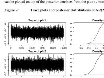
diagnostics in the coda package. For example, the trace plots in Figure 2 of the model parameters can be obtained after converting the posterior simulations to anmcmctype object:
> library("coda")
> param.mcmc <- as.mcmc(ar2$sims.matrix[,theta]) > plot(param.mcmc)
In the appendix of this paper, we illustrate how the density function of prior distributions can be plotted on top of the posterior densities from theplot.mcmcfunction.
Figure 2: Trace plots and posterior distributions of AR(2) model parameters
0 2000 4000 6000 8000 10000
−0.5
−0.3
−0.1
0.1
Iterations
Trace of phi1
−0.5 −0.4 −0.3 −0.2 −0.1 0.0 0.1
0
1
2
3
4
5
N = 10000 Bandwidth = 0.01314
Density of phi1
0 2000 4000 6000 8000 10000
−0.5
−0.3
−0.1
Iterations
Trace of phi2
−0.5 −0.4 −0.3 −0.2 −0.1 0.0 0.1
0
1
2
3
4
5
N = 10000 Bandwidth = 0.01311
Density of phi2
0 2000 4000 6000 8000 10000
0.0018
0.0024
Trace of sigma
0.0016 0.0018 0.0020 0.0022 0.0024 0.0026
0
1000
2500
Density of sigma
anal-ysis, these are typically summarised by using posterior means (as parameter estimates) and posterior standard deviations (as measures of uncertainty), which we calculated using
thesummary.mcmccommand in the coda package. For all AR models, the posterior
means ofσare around 0.002 with much lower standard deviations than in their prior dis-tributions. In all models, the posterior means ofφjat lower values ofjwere below zero,
indicating negative autocorrelation for these lags. Estimates ofφj, forj >5, tend to be
close to zero, signifying that the association betweenytandyt−jbecomes weak at larger
values ofj.
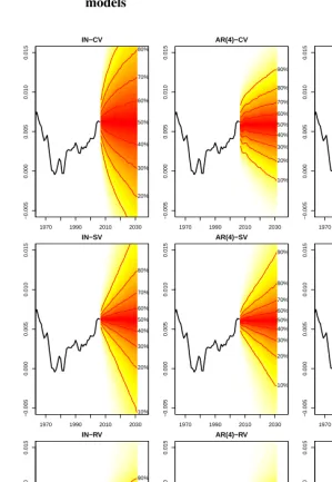
Posterior predictive plots of the forecastedrtfrom the IN, AR(4) and AR(8) models
are illustrated in the top row of Figure 3, where the darkest shades correspond to higher probability masses of the posterior distributions. Contour lines are also plotted at each decile. Forecasts from the simple independent normal (IN) model resulted in a higher level of uncertainty in future values than did any of the AR models. As autoregressive parameters were added to the independent normal model, the posterior predictive distri-bution became comparatively narrower.
Plots of the posterior predictive distributions can be replicated using thefanplot pack-age (Abel 2012) in R and the MCMC results stored in abugsobject:
> ynew.mcmc <- ar2$sims.list$y.new
> rnew.mcmc <- apply(ynew.mcmc, 1, diffinv, xi = r[166]) > rnew.mcmc <- t(rnew.mcmc[-1,])
> library("fanplot")
> rnew.pn <- pn(sims = rnew.mcmc, start = 2008) > plot(r, ylim = range(r), xlim = c(1970, 2040)) > fan(rnew.pn)
> lines(r)
The first three lines of this code use they.new[t]variables in the BUGS model and the last observed value ofrtto derive the simulated values of posterior predictive distribution
via thediffinvfunction. The rest of the code calculates the percentiles of the posterior predictive distributions forrtwith thepnfunction and then plots the percentile object
Figure 3: Posterior predictive plots of population growth rates from selected constant variance, stochastic volatility and random variance shift models
IN−CV
Time 1970 1990 2010 2030
−0.005 0.000 0.005 0.010 0.015 10% 20% 30% 40% 50% 60% 70% 80% AR(4)−CV Time 1970 1990 2010 2030
−0.005 0.000 0.005 0.010 0.015 10% 20% 30% 40% 50% 60% 70% 80% 90% AR(8)−CV Time 1970 1990 2010 2030
−0.005 0.000 0.005 0.010 0.015 10% 20% 30% 40% 50% 60% 70% 80% 90% IN−SV Time 1970 1990 2010 2030
−0.005 0.000 0.005 0.010 0.015 10% 20% 30% 40% 50% 60% 70% 80% 90% AR(4)−SV Time 1970 1990 2010 2030
−0.005 0.000 0.005 0.010 0.015 10% 20% 30% 40% 50% 60% 70% 80% 90% AR(8)−SV Time 1970 1990 2010 2030
4.2 Individual stochastic volatility models
Nine SV models were considered for the differenced population growth rate. The SV extension replaces theσ2term in the AR models with time dependent variancesσ2
t. As
specified in (5), this results in three new parametersψ0,ψ1 andτ, as well as values of htat each time point. Weakly informative prior distributions were also assigned to the
new parameters: e−ψ0 ∼Gamma(10−6,10−6), ψ
1 ∼ U(−0.999,0.999) andτ−2 ∼
Gamma(0.01,0.01). The BUGS models were again produced usingtsbugspackage. For example, a BUGS model for an AR(2)-SV process was created in R:
> sv2.bug <- sv.bugs(y, ar.order=2, k=25, beg=9, sv.mean.prior2 =
"dgamma(0.000001,0.000001)",
sv.ar.prior2 = "dunif(-0.999, 0.999)") > print(sv2.bug)
model{ #likelihood for(t in 9:190){
y[t] ~ dnorm(y.mean[t], isigma2[t]) isigma2[t] <- exp(-h[t])
h[t] ~ dnorm(h.mean[t], itau2) }
for(t in 9:190){
y.mean[t] <- phi1*y[t-1] + phi2*y[t-2] }
for(t in 9:9){
h.mean[t] <- psi0 }
for(t in 10:190){
h.mean[t] <- psi0 + psi1*(h[t-1]-psi0) }
#priors
phi1 ~ dnorm(0,1) phi2 ~ dnorm(0,1)
psi0.star ~ dgamma(0.000001,0.000001) psi0 <- -log(psi0.star)
#forecast
for(t in 166:190){ y.new[t] <- y[t] }
}
In the first loop of the BUGS model, the likelihood of the AR(2)-SV model is defined in a similar fashion as that of the constant variance equivalent shown previously. However, the precision term foryt,isigma2[t]has a index allowing for a variation over time. This
is formed by a transformation of the volatility processh[t]. In the second loop the AR(2) mean process is set up. In the third and fourth loops the mean level of the volatility process is given an AR(1) process for all but the initial data point. The likelihood part of the BUGS code is followed by the prior distributions which are specified in thesv.bugscommand to take the distributions presented at the beginning of this subsection (the default values for these arguments are different). Finally, a new set of variables is created to record the forecasted values. Plots of the MCMC traces, posterior and prior distributions of the AR(2)-SV model are shown in the appendix.
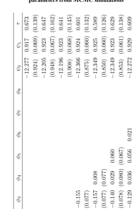
As with the constant variance models, the fitting of the parameters for the SV mod-els by OpenBUGS were run from R, allowing MCMC diagnostics checks and summary statistics of the posterior distributions to be easily obtained. The posterior means and standard deviations of the parameters in the nine SV models are presented in Table 1. Estimates of autoregressive parameters tend to be close to zero for mostφjwith the
ex-ception ofj = 2andj = 3. The posterior means ofψ0, the average volatility level, are
similar across all models. The corresponding values of the variance (eψ0) are very similar
to those for the AR models with constant variance. Posterior means forψ1, representing
the autocorrelation between a current level of volatility and that of a previous year, are all close to 0.92. This indicates a strong positive autocorrelation in the volatility levels ofrt.
Table 1: Posterior means (standard deviations) of stochastic volatility model parameters from MCMC simulations
The posterior distributions for theσtparameters, obtained by transforming the
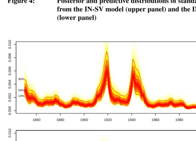
preci-sion values (isigma2[t]from OpenBUGS), are plotted in the upper panel of Figure 4 for the independent normal model with stochastic volatility (IN-SV). These were pro-duced in a similar fashion as the forecast fans in Figure 3. Inspection of this plot reveals a number of features. First, the estimated standard deviations decrease throughout most of the observed period. Volatility is at its lowest level in 2001, prior to a increase in sub-sequent years leading up to the last observation, marked by the vertical line. Second, the estimated standard deviations are highest during the 1918 influenza pandemic and war periods. During these years, the 10th percentiles of the estimated standard deviation are higher than the 90th percentiles for 2007. Finally, the median and width of the predictive distributions gradually increases over time.
Figure 4: Posterior and predictive distributions of standard deviation (σt)
from the IN-SV model (upper panel) and the IN-RV model (lower panel)
1860 1880 1900 1920 1940 1960 1980 2000 2020
0.000
0.002
0.004
0.006
0.008
0.010
10% 50% 90%
10% 50% 90%
1860 1880 1900 1920 1940 1960 1980 2000 2020
0.000
0.002
0.004
0.006
0.008
0.010
10% 50% 90% 10%
Posterior predictive plots of the forecastedrtfrom the IN-SV, AR(4)-SV and
AR(8)-SV models are presented in the middle row of Figure 3. Comparisons between models with SV terms reveal that uncertainty in forecastedrtis reduced through the addition of
autoregressive parameters, as was the case with the AR models with constant variance. However, forj > 3, the reductions in uncertainty were minimal as the values of φj
remained close to zero. Comparison of the forecasted population growth rates between the selected individual models with constant variance and the SV models (between the top and middle row in Figure 3) demonstrates a different shape in the forecast fans, caused by a combination of lowerφvalues and additional terms for a non-constant variance in the SV models. The inter-decile ranges of the predictive distributions in the SV models increase at a steady rate. The corresponding contour lines in the constant variance models, on the other hand, tend to spread quickly (depending on the order of the AR model) and then continue to widen at a steady but slower rate. For the IN model, the inclusion of the SV terms reduces the width of the predictive distribution, as illustrated in 2032 where the difference between the 90th and 10th percentile is 0.028 for the IN-CV model compared to 0.023 for the IN-SV model. This is because the SV model acknowledges the recently observed low volatility in its forecast.
4.3 Individual random variance shift models
As with the SV models, RV models allow for a time dependent variance ofyt. The RV
model replaces theψ0,ψ1,τandhtterms in the SV models with time constant parameters andλ, and time varying parametersβtandδt; see (6). For the additional parameters
in the RV model, we assigned the following prior distributions: βt ∼ N(0, λ2), δt ∼
Bernoulli()andλ−2∼Gamma(0.01,0.01). The prior distribution for∼Beta(1,100),
where Beta(a,b) denotes a beta distribution with shape parameteraand scale parameter
b, which is set to produce a low probability of a random variance shift. This reflects our prior belief that variance shifts should be relatively rare events.
Scripts to fit the models in OpenBUGS were produced using therv.bugscommand in thetsbugspackage. For example, the AR(2)-RV model was created in R:
> rv2.bug <- rv.bugs(y, ar.order=2, k=25, beg=9) > print(rv2.bug)
model{ #likelihood for(t in 9:190){
h[t] <- 2*lsig[t] }
for(t in 9:190){
y.mean[t] <- phi1*y[t-1] + phi2*y[t-2] }
lsig[9] <- -0.5*log(isig02) for(t in 10:190){
lsig[t] <- lsig[t-1]+(delta[t]*beta[t]) delta[t] ~ dbern(epsilon)
beta[t] ~ dnorm(0,ilambda2) }
#priors
phi1 ~ dnorm(0,1) phi2 ~ dnorm(0,1)
isig02 ~ dgamma(0.000001,0.000001) sig0 <- pow(isig02,-0.5)
epsilon ~ dbeta(1, 100) ilambda2 ~ dgamma(0.01,0.01) lambda <- pow(ilambda2,-0.5) #forecast
for(t in 166:190){ y.new[t] <- y[t] }
}
In the first loop of the BUGS code above, the likelihood of the AR(2)-RV model is defined similarly to the SV equivalent. However, the volatility,h[t], which monitored for com-parative purposes, is derived from transforming the logarithm of the standard deviation,
lsig[t]. This variable is set up in the last loop of the likelihood and is equivalent the logarithmic transformation of (6). Preceding the final in the likelihood part of the BUGS code is a transformation to the logarithmic scale of the standard deviation for the prior distribution defined by isig02. This prior is required in order to initiate subsequent variation levels and random shifts. As with previous BUGS code, the prior distributions are specified after the likelihood. Therv.bugscommand takes the prior distributions stated in the top of this subsection as default values. Finally, a new set of variables are created to record the forecasted values. Plots of the MCMC traces, posterior and prior distributions of the AR(2)-RV model are shown in the appendix.
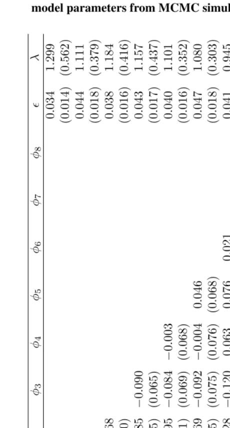
are presented in Table 2. Again, the estimates of the autoregressive parameters are close to zero for mostφj with the exception of j = 2andj = 3. The posterior means of,
i.e., the probability of a variance shift, are similar across all models with around a 4% chance of a variance shift in any given year during the observed period. Theλparameter, representing the magnitude (on the log scale) of average variance shifts, also remains relatively constant across all models.
The posterior distributions for theσt parameters are plotted in the lower panel of
Figure 4 for the independent normal model with random variance shifts (IN-RV). In com-parison to the SV plot in the upper panel, the standard deviations shift according to the
δtexhibit considerably narrower posterior distributions during periods of low volatility.
In the first period up to 1858, the standard deviation is at a relatively high level, before a downward shift, followed by a period of stability at a lower level. The standard deviations increase dramatically during the times of the two wars and the 1918 influenza pandemic. The posterior distributions of the standard deviations immediately after the Second World War are slightly lower than during the conflict period. In the early 1950s the standard deviations narrow considerably and with a lower median level. The upper deciles of the predicted posterior standard deviations from the RV model, in the future time period, are much lower than those of the SV model.
Posterior predictive plots of the forecastedrtfrom the IN-RV, AR(4)-RV and
Table 2: Posterior means (standard deviations) of random variance shift model parameters from MCMC simulations
4.4 Model-averaged forecasts
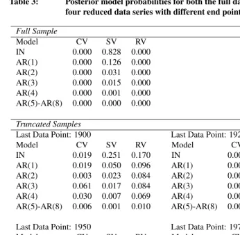
We estimated posterior probabilities,f(m|y{T}), for all models, using the approach de-scribed in Section 3.5. These are displayed in the top panel of Table 3. Note, the posterior probabilities for the models with AR component of order 5 or higher were very close to zero and hence are aggregated. A replicable demonstration of the calculations, performed in R using thetsbridgepackage (Abel, G.J. and Wong, J.T.S. 2013), is provided in the online supplementary materials.
Over all 27 models, the posterior model probabilities give strong support both the IN-SV model and the AR(1)-SV model (posterior probabilities of 0.828 and 0.126 re-spectively). Other SV models have some small amount of support. All models with a constant variance and random variance shift terms appear very unlikely with posterior model probabilities close to zero.
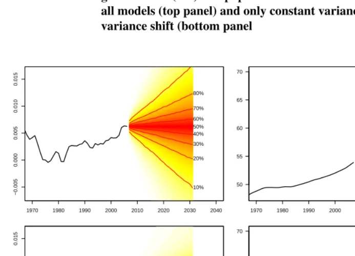
The predictive probability distributions ofrt, averaged over all models, are presented
in the top left hand panel of Figure 5. Because a sample from the posterior of probabil-ity distribution of each individual model is generated in the analysis, calculation of the averaged predictive probability distribution over all models is straightforward. Not sur-prisingly, this plot strongly resembles the IN-SV model forecast in Figure 3, for which large posterior model probabilities were obtained. However, one should keep in mind that it also includes a small amount of information from other SV models. On the top right hand panel of Figure 5, we present the resulting population forecasts from the predictive probability distributions ofrt. Our results provide a median predictive population of 62.9
million in 2032 with the 10th percentile at 55.2 million and the 90th percentile at 71.6 million.
A considerable contribution in the width of the 80% prediction intervals in the top panel of Figure 5 are generated by large tails in the forecast distributions, represented by the lighter, yellow colours. For example, the 60% prediction interval for the population in 2032 (9.0 million) is almost half the size of the 80% prediction interval (16.4 million). We found that smaller tails of forecasted distributions are produced if we dropped all stochastic volatility models from the anlaysis. These are shown in the bottom panel of Figure 5, where the medians are very close to those produced under all models. Forecasts are based predominately on a combination of the AR(2)-RV and IN-RV models with posterior probabilities of 0.558 and 0.440 respectively.
The decision to only consider RV models to account for non-constant variance might be of interest to potential user for a couple of reasons. First, the wider forecast distribu-tions from the inclusion of the SV models originate in the different specification of the time-varying variance term,σt. In the SV models the size of the tails of the forecasted
changes in the volatility during and between the wars. In contrast, in the RV models the future uncertainty in the forecasted distribution is predominately dictated by the estimate ofσT in the last observed period of the differenced series. As the estimated level in the
last period is at a historic low, see Figure 4, the smaller variance is carried through to the forecast. The RV model does allow for future increases (or decreases) from this estimated small variance, viathe probability of a shift. However, as shown in Table 2 these proba-bilities were relatively low. Second, as illustrated in the next section, for recent in-sample forecasts made in low volatility periods they appear to be better calibrated.
Figure 5: Joint predictive probability distribution of the model averaged growth rates (left) and population forecast in millions (right) over all models (top panel) and only constant variance and random variance shift (bottom panel
Time
1970 1980 1990 2000 2010 2020 2030 2040
−0.005
0.000
0.005
0.010
0.015
10% 20% 30% 40% 50% 60% 70% 80% 90%
Time
1970 1980 1990 2000 2010 2020 2030 2040 50
55 60 65 70
10% 20% 30% 40% 50% 60% 70% 80% 90%
1970 1980 1990 2000 2010 2020 2030 2040
−0.005
0.000
0.005
0.010
0.015
10% 20% 30% 40% 50% 60% 70% 80% 90%
1970 1980 1990 2000 2010 2020 2030 2040 50
55 60 65 70
Table 3: Posterior model probabilities for both the full data series (top) and four reduced data series with different end points (bottom)
Full Sample
Model CV SV RV
IN 0.000 0.828 0.000
AR(1) 0.000 0.126 0.000
AR(2) 0.000 0.031 0.000
AR(3) 0.000 0.015 0.000
AR(4) 0.000 0.001 0.000
AR(5)-AR(8) 0.000 0.000 0.000
Truncated Samples
Last Data Point: 1900 Last Data Point: 1925
Model CV SV RV Model CV SV RV
IN 0.019 0.251 0.170 IN 0.000 0.661 0.073
AR(1) 0.019 0.050 0.096 AR(1) 0.000 0.079 0.004
AR(2) 0.003 0.023 0.084 AR(2) 0.000 0.107 0.001
AR(3) 0.061 0.017 0.084 AR(3) 0.000 0.051 0.008
AR(4) 0.030 0.007 0.069 AR(4) 0.000 0.012 0.002
AR(5)-AR(8) 0.006 0.001 0.010 AR(5)-AR(8) 0.000 0.002 0.001
Last Data Point: 1950 Last Data Point: 1975
Model CV SV RV Model CV SV RV
IN 0.000 0.476 0.000 IN 0.000 0.744 0.000
AR(1) 0.000 0.251 0.000 AR(1) 0.000 0.125 0.000
AR(2) 0.000 0.119 0.000 AR(2) 0.000 0.060 0.000
AR(3) 0.000 0.132 0.000 AR(3) 0.000 0.064 0.000
AR(4) 0.000 0.019 0.000 AR(4) 0.000 0.007 0.000
AR(5)-AR(8) 0.000 0.002 0.000 AR(5)-AR(8) 0.000 0.000 0.000
The RV models tend to have lower posterior probabilities than the SV models, espe-cially for longer series, as they require considerably more parameters in the specification of theσt2. In the SV models, theσ2t series are estimated using three time constant param-eters (ψ0,ψ1andτ) and anotherT time varyinghtparameters. The RV models has only
two time-constant variables (andλ) but twice the amount of time varying parameters in
δtandβt. The higher number of parameters tend to lead to a small posterior density for
poste-rior probabilities, when the observed data does not clearly support a variance-shift type structure. However, for the purposes of forecasting population, the RV models can poten-tially provide a more effective control for outlier events in the past data, such as war and epidemics.
5.
In-sample forecast validation
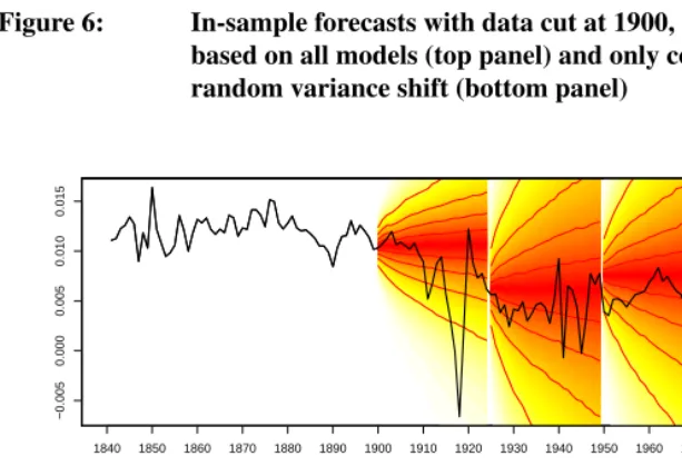
In this section, we show how the posterior model probabilities and associated forecasts change when four different time periods are used to fit the models: 1900, 1841-1925, 1841-1950 and 1841-1975. For each of the four time periods, we fitted the same 27 models described in Section 4 and then calculated the posterior model probabilities to produce model averaged forecasts. These in-sample forecasts were made for 25 years beyond the range of data used for fitting, to enable a comparison with actual observed rates, in order to validate the approach.
In the two bottom panels of Table 3, we present the posterior model probabilities for all 27 models fitted to each of the four time periods described above. As with the full sample in the top panel, the low posterior probabilities for models with AR orders of 5 and higher were aggregated for presentation purposes. For the first set of models, based on population data from 1841-1900, we find the IN-SV model has the largest model probability of 0.251, followed by the IN-RV model, and then other SV and RV models. For this period, there was a small amount of support for the models with constant variance. For the second forecast, based on data from 1841-1925, the model probabilities indicate a large support for the IN-SV models with a probability of 0.661. The third forecast, based on data from 1841-1950, resulted in the large model probabilities for IN-SV and AR(1)-SV models as was the case for the final forecast based on data from 1841-1975. In comparison to the model probabilities for the full sample forecast presented in the upper panel of Table 3, the forecasts with end points 1925, 1950 and 1975 are similar in that they all have considerable model probabilities for SV models, especially the IN-SV for the longer series. In all cases, there was very little support for the constant variance models.
percentile of the predictive distribution. For the last forecast, we see the uncertainty de-creases somewhat, after the variance shifts to a period of relatively low volatility. Here, the observed data remain within the 30th and 70th percentiles.
The posterior predictive distributions for the four periods based only on constant vari-ance and random varivari-ance shift models are shown in the bottom panel of Figure 6. The forecasted distributions are wider than those based predominately on the SV models for data cut at 1925 and 1950, due to higher variances levels estimated in the RV models during these base years. In the case of the series ending in 1925, there are too few ob-servations beyond the war and pandemic to shift variance levels downwards, as suggested by models fitted to the entire data series (as in Figure 4). Conversely, as with the 2007 forecast in the previous section, they provide narrower forecasted distributions in low volatility periods. In the case of the forecast from the series ending in 1975 the forecast distribution appears to be better calibrated to future observed values that the forecasts based predominately on the SV models.
Figure 6: In-sample forecasts with data cut at 1900, 1925, 1950 and 1975 based on all models (top panel) and only constant variance and random variance shift (bottom panel)
Time
1840 1850 1860 1870 1880 1890 1900 1910 1920 1930 1940 1950 1960 1970 1980 1990 2000 2010
−0.005
0.000
0.005
0.010
0.015
10% 20% 30% 40% 50% 60% 70% 80% 90%
1840 1850 1860 1870 1880 1890 1900 1910 1920 1930 1940 1950 1960 1970 1980 1990 2000 2010
−0.005
0.000
0.005
0.010
0.015
6.
Conclusion
In this paper, we have explored the use of Bayesian models to forecast a single time series of population data in England and Wales from 1841 to 2007 forward to 2032. The key issue has been the specification of uncertainty in the forecasts. We have shown that both the forecasted medians and measures of uncertainly can differ considerably depending on the time series model used. This was reconciled by developing a Bayesian approach which combines forecasts from different models, with weights determined by how well models fit the observed data. We found that models which allow the underlying variance to shift at particular time points fitted the observed data well. They also provided a realistic assessment of forecast uncertainty which balances recent levels of variability with the probability that variance shifts may occur in the future, at a rate which is estimated based on the historical prevalence of such events.
The contributions of this paper are threefold. First, we have presented the Bayesian approach to time series forecasting for use in population applications. The computational steps required to estimate the model parameters have also been illustrated. Second, we have shown how Bayesian models are capable of including multiple sources of uncer-tainty. In particular, we extended standard autoregressive time series models to include stochastic volatility, random variance shifts and model averaging. In this paper, we have introduced these ideas by using relatively simple time series data, in order to develop a framework for incorporating Bayesian methods to produce population forecasts, and to gain a good understanding of the benefits. The results show the limitations of using a sin-gle model, particularly in the specification of uncertainty. While the underlying inputs we have used in this paper are relatively simple, the results can be used to provide a bench-mark for specifying uncertainty in more complex projection situations that include, for example, age and demographic components of change (fertility, mortality and migration). These methods will also be valuable for forecasting other single demographic indicator variables, such as total fertility rates or life expectancies. Third, we have applied random variance shift models based on McCulloch and Tsay (1993), to forecast future popula-tion. We found these models, which to our knowledge have not previously been applied to demographic data, effectively controlled forecasts for the observed volatility.
King 2008; Raftery et al. 2013) and migration (Brierley et al. 2008; Bijak 2010; Raymer, J., Wi´sniowski, A., Forster, J.J., Smith, P.W.F. and Bijak, J. 2013) provide good starting points. However, as the projection models become more complex, the relative importance of expert opinion will increase (see Bijak and Wi´sniowski (2010) ). Fortunately, the Bayesian approach allows data and uncertainty in parameters and model choice to be fully quantified using probability distributions. In our implementation, prior distributions, which was kept weakly informative, had minimal influence on the final forecasts. This is not likely to be the case with more detailed forecasts, or in situations where the availability of data is lacking.
In conclusion, this work is relevant as most statistical agencies still rely on ‘high’ and ‘low’ variants to communicate uncertainty around their principal population projec-tions. Such variants have a number of drawbacks with the most prominent being a lack of specificity regarding the probability range of the high, low or even principal variants (for discussion, see Keilman, Pham, and Hetland (2002) or Lutz and Goldstein (2004)). In response, demographers and statisticians have developed frequentist methods to calculate probabilistic forecasts that describe the uncertainly of future populations by relying on time series models, expert judgements or extrapolation of past forecast errors (Keilman 2001; Keilman, Pham, and Hetland 2002). Methods have also been developed to combine elements of each of these approaches, for example, the parameters from time series mod-els have been constrained according to expert opinions (Lee and Tuljapurkar 1994) or to target levels and age distributions of fertility and mortality (Lutz, Sanderson, and Scher-bov 2001). However, the use of Bayesian methods, which have the potential to bring all of these ideas together, are only recently gaining prominence in population forecasting (Bryant and Graham 2013; Raftery et al. 2012). We hope this paper illustrates some of the advantages of the Bayesian approach and motivates researchers to carefully consider not only if but how they include uncertainty in their forecasts.
7.
Acknowledgements
References
Abel, G.J. (2012). fanplot: Visualisations of sequential probability distributions. URL: http://cran.r-project.org/web/packages/fanplot/.
Abel, G.J. (2013). tsbugs: Create time series BUGS models. URL: http://cran.r-project.org/web/packages/tsbugs/.
Abel, G.J. and Wong, J.T.S. (2013). tsbridge: Calculate normalising constants for
Bayesian time series models.URL: http://cran.r-project.org/web/packages/tsbridge/.
Ahlburg, D. (1987). Population Forecasts for South Pacific Nations using Au-toregressive Models 1985-2000. Journal of Population Research 4(2): 157–167.
doi:10.1007/BF03029414.
Alho, J.M. and Spencer, B.D. (2005). Statistical Demography and Forecasting. New York, USA: Springer.
Alho, J.M. and Spencer, B.D. (1985). Uncertain Population Forecasting. Journal of the
American Statistical Association80(390): 306–314.doi:10.2307/2287887.
Alkema, L., Raftery, A.E., Gerland, P., Clark, S.J., and Pelletier, F. (2012). Estimating trends in the total fertility rate with uncertainty using imperfect data: Examples from West Africa. Demographic Research 26(15): 331–362.
doi:10.4054/DemRes.2012.26.15.
Alkema, L., Raftery, A.E., Gerland, P., Clark, S.J., Pelletier, F., Buettner, T., and Heilig, G.K. (2011). Probabilistic Projections of the Total Fertility Rate for All Countries.
Demography48(3): 815–839.
Anderson, M. (ed.) (1996). British Population History: From the Black Death to the
Present Day. Cambridge, United Kingdom: Cambridge University Press.
Bijak, J. (2010). Forecasting International Migration in Europe: A Bayesian View. Dor-drecht, Netherlands: Springer, 1st ed.
Bijak, J. and Wi´sniowski, A. (2010). Bayesian forecasting of immigration to selected European countries by using expert knowledge. Journal of the Royal
Statistical Society: Series A (Statistics in Society) 173(4): 775–796. doi:10.1111/
j.1467-985X.2009.00635.x.
Brierley, M.J., Forster, J.J., McDonald, J.W., and Smith, P.W.F. (2008). Bayesian Es-timation of Migration Flows. In: Raymer, J. and Willekens, F. (eds.). International
Migration in Europe. Chichester, United Kingdom: Wiley: 149–174.
population estimation using multiple data sources. Bayesian Analysis 8(2): 1–34.
doi:10.1214/13-BA820.
Chatfield, C. (2003). The Analysis of Time Series: An Introduction. Texts in Statistical Science. Boca Raton, USA: Chapman and Hall/CRC, 6th ed.
Coleman, D. and Salt, J. (1992).The British Population: Patterns, Trends, and Processes. Oxford, USA: Oxford University Press.
Gelman, A., Carlin, J.B., Stern, H.S., and Rubin, D.B. (2003). Bayesian Data Analysis. Boca Raton, USA: Chapman & Hall/CRC, 2nd ed.
Girosi, F. and King, G. (2008). Demographic Forecasting. Princeton, USA: Princeton University Press.
Heilig, G., Buettner, T., Li, N., Gerland, P., Alkema, L., Chunn, J., and Raftery, A. (2010). A stochastic version of the United Nations World Population Prospects: Method-ological improvements by using Bayesian fertility and mortality projections. Lisbon, Portugal: Joint Eurostat/UNECE Work Session on Demographic Projections. URL: www.unece.org/fileadmin/DAM/stats/documents/ece/ces/ge.11/2010/wp.14.e.pdf.
Hinde, A. (2003).England’s Population: A History since the Domesday Survey. London, United Kingdom: Arnold Publication.
Hoeting, J.A., Madigan, D., Raftery, A.E., and Volinsky, C.T. (1999). Bayesian Model Averaging: A Tutorial.Statistical Science14(4): 382–401. doi:10.2307/2676803.
Keilman, N. (2001). Demography. Uncertain population forecasts. Nature412(6846): 490–491.doi:10.1038/35087685.
Keilman, N. and Pham, D.Q. (2004). Time Series Based Errors and Empirical Errors in Fertility Forecasts in the Nordic Countries. International Statistical Review/Revue
Internationale de Statistique72(1): 5–18. doi:10.2307/1403839.
Keilman, N., Pham, D.Q., and Hetland, A. (2002). Why population forecasts should be probabilistic - illustrated by the case of Norway. Demographic Research6: 409–454.
doi:10.4054/DemRes.2002.6.15.
Keyfitz, N. (1991). Uncertainty in National Population Forecasting: Issues, Backgrounds, Analyses, Recommendations. Population Studies: A Journal of Demography 45(3): 545–546.doi:10.1080/0032472031000145786.
Lee, R.D. (1998). Probabilistic Approaches to Population Forecasting. Population and
Development Review24: 156–190.doi:10.2307/2808055.
States: Beyond High, Medium, and Low.Journal of the American Statistical Associa-tion89(428): 1175–1189.doi:10.2307/2290980.
Lunn, D., Spiegelhalter, D., Thomas, A., and Best, N. (2009). The BUGS project: Evolution, critique and future directions. Statistics in Medicine28(25): 3049–3067.
doi:10.1002/sim.3680.
Lutz, W. and Goldstein, J.R. (2004). Introduction: How to Deal with Uncertainty in Pop-ulation Forecasting? International Statistical Review/Revue Internationale de
Statis-tique72(1): 1–4.doi:10.1111/j.1751-5823.2004.tb00219.x.
Lutz, W., Sanderson, W., and Scherbov, S. (2001). The end of world population growth.
Nature412(6846): 543–545.
McCulloch, R.E. and Tsay, R.S. (1993). Bayesian Inference and Prediction for Mean and Variance Shifts in Autoregressive Time Series.Journal of the American Statistical
Association88(423): 968–978.doi:10.1080/01621459.1993.10476364.
Meng, X.L. and Wong, W.H. (1996). Simulating Ratios of Normalizing Constants via a Simple Identity: A Theoretical Exploration. Statistica Sinica6: 831–860. URL: http://www3.stat.sinica.edu.tw/statistica/oldpdf/A6n43.pdf.
O’Hagan, A. and Forster, J.J. (2004). Bayesian Inference. Kendalls Advanced Theory of Statistics. London, United Kingdom: Arnold Publication, 2nd ed.
Pedroza, C. (2006). A Bayesian forecasting model: predicting U.S. male mortality. Bio-statistics7(4): 530–550.doi:10.1093/biostatistics/kxj024.
Pflaumer, P. (1992). Forecasting US population totals with the Box-Jenkins ap-proach. International Journal of Forecasting 8(3): 329–338. doi:10.1016/
0169-2070(92)90051-A.
Plummer, M., Best, N., Cowles, K., and Vines, K. (2006). CODA: Conver-gence diagnosis and output analysis for MCMC. R News 6(1): 7–11. URL: http://cran.r-project.org/doc/Rnews/Rnews_2006-1.pdf.
Raftery, A.E., Chunn, J.L., Gerland, P., and Sevˇcíková, H. (2013). Bayesian probabilistic projections of life expectancy for all countries.Demography50(3): 777–801.
Raftery, A.E., Li, N., Ševˇcíková, H., Gerland, P., and Heilig, G.K. (2012). Bayesian probabilistic population projections for all countries. Proceedings of the
Na-tional Academy of Sciences of the United States of America 109(35): 13915–21.
doi:10.1073/pnas.1211452109.
Modelling of European Migration: Background, Specification and Results.NORFACE
Migration Discussion Paper(4).
Raymer, J., Wi´sniowski, A., Forster, J.J., Smith, P.W.F. and Bijak, J. (2013). Integrated Modeling of European Migration. Journal of the American Statistical Association
108(503): 801–819.doi:10.1080/01621459.2013.789435.
Saboia, J.L.M. (1974). Modeling and Forecasting Populations by Time Series: The Swedish Case.Demography11(3): 483–492. doi:10.2307/2060440.
Sturtz, S., Ligges, U., and Gelman, A. (2005). R2WinBUGS: a package for running WinBUGS from R.Journal of Statistical Software12(3): 1–16.
Tayman, J., Smith, S.K., and Lin, J. (2007). Precision, bias, and uncertainty for state pop-ulation forecasts: an exploratory analysis of time series models. Population Research
and Policy Review26(3): 347–369.doi:10.1007/s11113-007-9034-9.
Tuljapurkar, S. (1999). Validation, probability-weighted priors, and information in stochastic forecasts. International Journal of Forecasting 15(3): 259–271.
doi:10.1016/S0169-2070(98)00082-X.
Appendix
Adding a plot of prior distributions to those generated from theplot.mcmccommand in the coda package is not straight forward. In this appendix we illustrate some R code to enable the prior and posterior distributions to appear on the same plot for each of the model types illustrated in this paper.
Thenodesfunction in thetsbugspackage provides adata.frameon the parameters used in the prior part of the BUGS script. Using thear2object (see Section 4.1) we may illustrates its output,
> pp <- nodes(ar2.bug, part="prior") > pp
name type dt beg end stoc id dist param1 param2
1 phi1 ~ dnorm(0,1) NA NA 1 2 dnorm 0.000000 1.000000
2 phi2 ~ dnorm(0,1) NA NA 1 3 dnorm 0.000000 1.000000
3 isigma2 ~ dgamma(0.000001,0.000001) NA NA 1 4 dgamma 0.000001 0.000001
4 sigma <- pow(isigma2,-0.5) NA NA 0 5 <NA> NA NA
The MCMC simulations for these parameters, stored in thear2object can be extracted after defining our parameter set,theta, as those parameters that have prior distributions directly defined in the BUGS script,
> pp <- subset(pp, stoc==1) > theta <- pp$name
> j <- length(theta)
> param.mcmc <- as.mcmc(ar2$sims.matrix[,theta]).
These simulations, that are nowmcmctype objects, can be plotted using theplot.mcmc
command,
> par(mfrow=c(j,2))
> plot(param.mcmc, auto.layout=FALSE).
To add the posterior densities to the plots, we consider each density plot in the second column within theforloop below,
> par(mfrow=c(j,2))
> for(i in 1:j){ par(mfg=c(i,2))
densplot(param.mcmc[,i], yaxt="n", xaxt="n") xx <- par()$usr[1:2]
xx <- seq(min(xx) ,max(xx), length=1000) f <- match.fun(pp$dist[i])
if(pp$dist[i]=="dnorm") pp$param2[i] <- 1/sqrt(pp$param2[i]) lines(xx, f(xx, pp$param1[i], pp$param2[i]), col="orange") }
Within the loop, we first select the plotting area using themfggraphical parameter, then overlay the exiting plot with the same posterior density. Second, using theusrgraphical parameter, information on the range of the x-axis is first saved, and then used to create a sequence of numbers within the minimum and maximum values. Third, the distribution function of the prior parameter is stored as function labelledf. In addition, if this func-tion isdnormthe second, precision parameter, stored in theppobject is converted to a standard deviation. Finally, the density of the given prior distributions and its parameters are calculated for values over the range of the x-axis and plotted as a orange line. The output from this sequence of code for thear2object is shown in Figure A-1.
The code above can also be used to plot prior and posterior distributions for the stochastic volatility and random variance shifts models. This can be done after defin-ingppas the BUGS script produced in the paper, fromsv2.bugorrv2.bugand the
param.mcmcobject as the corresponding MCMC simulation results, stored insv2or
Figure A-1: Trace plots, posterior and prior (orange) densities of AR(2) model parameters
0 2000 4000 6000 8000 10000
−0.5
−0.3
−0.1
0.1
Iterations
Trace of phi1
−0.5 −0.4 −0.3 −0.2 −0.1 0.0 0.1
0
1
2
3
4
5
Density of phi1
N = 10000 Bandwidth = 0.01314
0 2000 4000 6000 8000 10000
−0.5
−0.3
−0.1
Iterations
Trace of phi2
−0.5 −0.4 −0.3 −0.2 −0.1 0.0 0.1
0
1
2
3
4
5
Density of phi2
N = 10000 Bandwidth = 0.01311
0 2000 4000 6000 8000 10000
150000
250000
350000
Trace of isigma2 Density of isigma2
150000 200000 250000 300000 350000
0.0e+00
1.0e−05
N = 10000 Bandwidth = 0.01314
Figure A-2: Trace plots, posterior and prior (orange) densities of AR(2)-SV model parameters
0 2000 4000 6000 8000 10000
−0.4
0.1
Iterations
Trace of phi1
−0.4 −0.2 0.0 0.2 0.4
0
2
4
Density of phi1
N = 10000 Bandwidth = 0.01498
0 2000 4000 6000 8000 10000
−0.4
0.1
Iterations
Trace of phi2
−0.5 −0.4 −0.3 −0.2 −0.1 0.0 0.1 0.2
0
2
4
Density of phi2
N = 10000 Bandwidth = 0.01325
0 2000 4000 6000 8000 10000
0
1200000
Iterations
Trace of psi0.star Density of psi0.star
0 500000 1000000 1500000
0.0e+00
0 2000 4000 6000 8000 10000
0.6
0.9
Iterations
Trace of psi1
0.6 0.7 0.8 0.9 1.0
0
4
8
Density of psi1
N = 10000 Bandwidth = 0.01083
0 2000 4000 6000 8000 10000
2
6
Trace of itau2
0 2 4 6 8 10
0.0
0.3
Density of itau2
N = 10000 Bandwidth = 0.01498
N = 10000 Bandwidth = 0.01325
Figure A-3: Trace plots, posterior and prior (orange) densities of AR(2)-RV model parameters
0 2000 4000 6000 8000 10000
−0.3
0.1
Iterations
Trace of phi1
−0.4 −0.3 −0.2 −0.1 0.0 0.1 0.2
0
2
4
Density of phi1
N = 10000 Bandwidth = 0.0121
0 2000 4000 6000 8000 10000
−0.4
0.0
Iterations
Trace of phi2
−0.4 −0.3 −0.2 −0.1 0.0 0.1
0
3
6
Density of phi2
N = 10000 Bandwidth = 0.01012
0 2000 4000 6000 8000 10000
0
250000
Iterations
Trace of isig02 Density of isig02
0 50000 150000 250000
0.0e+00
0 2000 4000 6000 8000 10000
0.02
0.12
Iterations
Trace of epsilon
0.00 0.02 0.04 0.06 0.08 0.10 0.12
0
15
Density of epsilon
N = 10000 Bandwidth = 0.002683
0 2000 4000 6000 8000 10000
0
2
4
Trace of ilambda2
0 1 2 3 4 5
0.0
0.6
Density of ilambda2
N = 10000 Bandwidth = 0.0121
N = 10000 Bandwidth = 0.01012