Multi-Reference Pseudo-Random Phase-Encoded Joint Transfrom Correlation

University of New Orleans University of New Orleans

ScholarWorks@UNO

ScholarWorks@UNO

University of New Orleans Theses and

Dissertations Dissertations and Theses

1-20-2006

Multi-Reference Pseudo-Random Phase-Encoded Joint Transfrom

Multi-Reference Pseudo-Random Phase-Encoded Joint Transfrom

Correlation

Correlation

Follow this and additional works at: https://scholarworks.uno.edu/td

Recommended Citation Recommended Citation

Mwatibo, Edward, "Multi-Reference Pseudo-Random Phase-Encoded Joint Transfrom Correlation" (2006). University of New Orleans Theses and Dissertations. 1033.

https://scholarworks.uno.edu/td/1033

This Thesis is protected by copyright and/or related rights. It has been brought to you by ScholarWorks@UNO with permission from the rights-holder(s). You are free to use this Thesis in any way that is permitted by the copyright and related rights legislation that applies to your use. For other uses you need to obtain permission from the rights-holder(s) directly, unless additional rights are indicated by a Creative Commons license in the record and/or on the work itself.

MULTI-REFERENCE PSEUDO-RANDOM PHASE-ENCODED JOINT TRANSFORM CORRELATION

A Thesis

Submitted to the Graduate Faculty of the University of New Orleans

in partial fulfillment of the requirements for the degree of

Master of Science in

Engineering

by

Edward Mwatibo

M.S. University of New Orleans, 2005

DEDICATION

I give my sincere love and thanks to my whole family especially my dear wife and my children,

for their endless love, unlimited caring, and understanding. I also highly appreciate the help extended by

ACKNOWLEDGMENTS

I would first like to express my gratitude to my advisor, Dr. Abdul Rahman Alsamman, for

giving me this opportunity to study with him. I appreciate his insightful guidance, patience,

encouragement, understanding and support during this research. I would also like to thank the other

members of my committee, Dr. Dimitrios Charalampidis and Mr. Kim Jovanovich, for the assistance

TABLE OF CONTENTS

LIST OF FIGURES ...iv

LIST OF TABLES ...vii

ABSTRACT ...viii

1 INTRODUCTION...1

1.1 Problem Description...2

1.2 Thesis Organization...2

2 OPTICAL PROCESSING ...4

2.1 Basic Optical Components ...4

2.2 Matched Filter Correlator...7

2.3 Joint Transform Correlator ...9

2.4 Fourier Plane Image Subtraction...13

2.5 Binary JTC ...15

2.6 Fringe-Adjusted JTC ...15

2.7 Phase-Encoded JTC ...17

3 RANDOM PHASE MASK...22

3.1 M-sequence...22

3.2 Two Dimensional Arrays ...26

3.2.1 Shift and add property...27

3.2.2 Array Auto-Correlation...30

3.2.3 Array Cross-Correlation ...30

3.3 Random Phase Mask Algorithm ...30

3.4 Comparison of Different encoding levels ...32

4 MULTI-REFERENCE PHASE ENDODED JTC...38

4.1 Multi-Reference Phase Encoded JTC Using Phase SLM Only ...42

4.2 Comparison of Correlation Output Results...46

4.3 Performance Evaluation...50

4.3.1 PSR /PCE Ratios for Different SLM Size ...51

4.3.2 PSR /PCE for varying SLM Size and Varying Joint Input Image...55

4.3.3 PSR /PCE for varying No of Input Images...59

4.4 Spatially Efficiency Evaluation...63

4.4.1 Comparison of Correlation Outputs ...63

5 CONCLUSION...67

6 REFERENCES ...69

LIST OF FIGURES

Figure 2-1: A Matched Filter based Correlator...8

Figure 2-2: Joint Transform Correlator ...10

Figure 2-3: Joint Input Image...11

Figure 2-4: Correlation Output ...12

Figure 2-5: JTC Employing Fourier Plane Image Subtraction...14

Figure 2-6: Fringe-Adjusted JTC ...17

Figure 2-7: Correlation output of a Phase Encoded JTC ...19

Figure 2-8: Phase Encoded JTC...21

Figure 3-1: Generalized Generator...23

Figure 3-2: Addition of Two Sequences ...28

Figure 3-3: Example of m-array...29

Figure 3-4: Formulation of Random Phase Mask ...32

Figure 3-5: Histogram of binary encoding (m=2)...33

Figure 3-6: Histogram of ternary encoding (m=3)...34

Figure 3-7: Histogram of level five encoding (m=5)...34

Figure 3-8: Correlation Outputs for Image created with a Random phase mask (m=2)...35

Figure 3-9: Correlation Outputs for Image created with a Random phase mask (m=3)...36

Figure 3-10: Correlation Outputs for Image created with a Random phase mask (m=5)...36

Figure 3-11: Correlation Outputs for Image created with a Random phase mask ...37

Figure 4-1: Multi-Reference Phase Encoded JTC ...40

Figure 4-2: Joint Input Image...41

Figure 4-3: Output of JTC...41

Figure 4-4: Joint Input Image...43

Figure 4-5: Correlation Output of Modified JTC ...44

Figure 4-6: Multi-reference Phase Encoded JTC Using Phase SLM Only...46

Figure 4-7: Joint Input Image Correlation Outputs...47

Figure 4-8: First Reference Image Correlation Outputs ...48

Figure 4-9: Second Reference Image Correlation Outputs...49

Figure 4-10: Image of a Rose Flower ...50

Figure 4-11: Peak to Side lobe ratio estimation...50

Figure 4-12: PSR Vs SLM SIZE ...52

Figure 4-13: PCE Vs SLM Size ...52

Figure 4-14: Correlation Output Using Different SLM Size But Same Joint Input Image (a)128 x 128 (b) 256 x 256 ...53

Figure 4-15: Correlation Output Using Different SLM Size But Same Joint Input Image (a)512 x 512 (b) 1024 x 1024 ...54

Figure 4-16: PCE Vs Ratio of Joint Image to SLM Size...55

Figure 4-17: PSR Vs Ratio of Joint Image to SLM Size...56

Figure 4-19: Correlation Output Using Different SLM Size and Joint Input Image Size but Same

Image to SLM Size Ratio (a)64 x 64 / 512 x 512 (b) 128 x 128 / 1024 x 1024 ...58

Figure 4-20: PSR Vs No of Images...60

Figure 4-21: PCE Vs No of Images ...60

Figure 4-22: Correlation Output - One Reference Image...61

Figure 4-23: Correlation Output – Two Reference Images ...61

Figure 4-24: Correlation Output – Three Reference Images ...62

Figure 4-25: Correlation Output – Four Reference Images...62

LIST OF TABLES

ABSTRACT

We propose and demonstrate the superiority of using a phase SLM only in a multi-reference phase

encoded joint transform correlator(JTC) compared to an ordinary JTC. Maximal length sequences are

shifted to form two dimensional orthogonal arrays referred as m-arrays. The phase mask is used in one

step to encode multiple reference images and at the same time eliminate false correlation peaks through

power spectrum dispersion. A theoretical model of the implemented JTC is mathematically expressed

and explained in this thesis. Basic performance criteria, PSR (peak to side lobe ratio) and PCE (peak to

correlation energy), are used for comparative analysis, and their relationship to joint input image size and

1 INTRODUCTION

The development of optical components during the twentieth century has led to many advances

in the design of optical processing systems, which are used as data processing systems and to

complement computerized systems. The popularity of optical processing is mainly due to their

processing capabilities and immense parallelism.

Fourier optical signal processing is one of the oldest forms of optical signal processing, with a

history dating back to 1893 [1]. Its foundation is based on the ability of a lens to perform

two-dimensional (2D) Fourier transform. Since their introduction, optical processing systems have

successfully been utilized in a variety of areas including radar signal processing, optical pattern

recognition and target tracking.

There are two commonly used optical correlation techniques: The first is matched spatial filtering

optical correlation, developed by Vander Lugt [2] in 1964, and the second is the joint transform

correlation (JTC) proposed by Weaver and Goodman [3] in 1966. For real time applications, JTC is

preferred over Vander Lugt correlator because it does not require complex filtering or precise

alignment, but it suffers strong zero order term and has overlapping correlation peaks. To reduce these

effects, an increase in displacement between the images is required or an optical stop is introduced at

the center of the output plane, thus leading to a more inefficient use of the spatial area of the optical

beam.

Different architectures [4] have since been proposed to improve the JTC optical correlators in

performance and discrimination ability, especially in the presence of multiple input images. These

(JPS), like binary JTC [5], amplitude-modulated filter based JTC [6], and chip-encoded JTC [7] and

fringe-adjusted JTC [8]. Other methods that have been implemented to improve correlation

discrimination by reducing extraneous peaks include Fourier plane image subtraction [9] and phase

encoding input JTC technique [10, 11]. These systems are considerably more complex in design. None

of the proposed techniques in literature have attempted to improve the spatial inefficiency of the JTC

system.

1.1 P

D

In this thesis, we introduce a phase encoded JTC system that employs Pseudo-random phase

masks to encode multiple reference images in a JTC system. The phase masks are generated using

maximal length sequences (M-sequences), which are Pseudo-random sequences that are easy to

generate and have low autocorrelation and cross correlation side lobes. The system will be designed to

make exploit the parallelism inherent in the optical system and to multiplexing many reference images in

phase such that multiple correlations can be performed at the same time. A reference-encoding method

will be utilized to considerably simplify the architecture of the proposed system. The random phase

mask is used to improve the spatial efficiency by eliminating the spatial displacement between the input

and reference images. The actual phase encoding process is performed electronically a prior thus

removing the need for online encoding.

1.2 T

O

Chapter 2 provides a brief overview of optical processing and its advantages. It also includes a

summary of the main optical components and a description of the variant JTC architecture. Chapter 3

been used to create two-dimensional M-sequence arrays used for phase-encoding. Chapter 4 describes

the implementation details for the modified phase encoded JTC and investigates the effect of image size

and SLM size on the correlation output. Chapter 5 presents computer simulated results of the proposed

system. Finally, Chapter 6 concludes the thesis by summarizing the major results, analyzing some of the

2 OPTICAL PROCESSING

Compared to their electronic counterparts, optical system possess: a higher degree of

parallelism, a faster processing speed that is more suited for real time applications, immune to

electromagnet interference, and provide low-loss transmission with large bandwidth[12].

2.1 B

O

C

A vast development in optoelectronic devices in the last century has enabled the creation of

optical data processors. These devices are the fundamental key in the integration between electronics

and optical technology. Table 2-1 groups different optical components into four major categories: signal

generators, signal modulators, signal detectors and signal steering devices.

Category Device

Signal Generator LED (Light emitting diode)

VCSEL(Vertical cavity surface emitting laser)

Signal Modulator LCD (Liquid crystal display)

AOSLM (Acousto optic spatial light modulator)

EOLM (Electro optical light modulator)

Signal Detector CCD (Charged coupled device)

CMOS (Complementary metal-oxide semiconductor) detector

Signal Steering Device Mirrors

Prisms

Table 2-1: Examples of Opto-electronic Devices

All four categories (generation, modulation, steering and detection) are operative in the joint

transform correlation process.

• Signal generators

Light sources, which come in a huge array of sizes, shapes, and colors, are selected depending

on response speed required, bandwidth to be achieved and the type of application to be used

in. In optical processing, Laser diodes and LED (light emitting diodes) are the main types of

lighting sources used.

• Signal modulators: these devices are also known as spatial light modulators (SLMs).

The SLM is an opto-electronic input device that plays an important role in an optical processing

system by controlling light on a pixel-to-pixel basis. The SLM accepts the input data (pattern

information) from a digital input (host computer) and converts coherent light input from a laser

source into output data. Commercially, SLMs are classified using the following criteria [13]:

addressing methods; coherent light requirement; modulation scheme; quality of the input; setup

and hold time; other specifications include size, power consumption and range of temperature.

For a phase-only mode, the SLM encodes the input light beam with a phase such that it

produces the desired input data, which can be expressed as

( ) 0

( ) ( ) i r (1)

A r = A r eψ

where A r₀( ) is the complex amplitude of the beam incident on the SLM [14].

Although the use of SLMs increases the overall flexibility, they have the following disadvantages;

The most commonly used SLM types are Liquid Crystal Television (LCTV), Magneto-optic

SLM (MOSLM), and Deformable Mirror Device (DMD) [15].

• Signal steering devices 1. Mirrors

Optical beam steering is commonly accomplished via the use of mirrors and prisms. This kind of

combination tends to increase the size, weight and complexity of the optical system. Mirrors and

prisms control direction of light through reflection and refraction respectively.

2. Beam Splitters (BS)

Beam splitter is an optical device that is used to split a beam of light into two or more light

beams. It consists of partially transparent mirror (half–silvered) which allows part of the beam

light to reflect off while the other part goes through it. It is also referred to as Beam Combiner

when used to combine multiple beams into a single beam.

3. Lenses

Optical signal processing has relied heavily on the Fourier transform property of a lens, which

was discovered a century ago by German scientist E. Abbe [16]. Both the 2 D Fourier and its

inverse transform are performed by a converging lens, which also captures as much of the

source light beam as possible and transforms it into a collimated output.

• Signal detectors

Charged Coupled Device (CCD) Detector

W.S. Boyle and G.E. Smith of the Bell Laboratory [17] invented the Charged Coupled Device

(CCD) known as a square–law device in 1969. This device, which converts incident light into

The interface between the optical and electronic system in a JTC is provided by a combination

use of SLMs and CCDs. This opto-electronic interaction forms the basis of hybrid operation,

enabling an optimal achievement in terms of performance, speed and cost.

2.2 M

F

C

The fundamental theory of optical spatial filtering was introduced by Cheatham, Kohlenberg and

O’Nell [18]. Since then significant progress has been made in spatial filtering with Vander Lugt [2]

presenting an optical correlator using complex spatial filtering 1964. His system performed a correlation

between two functions f x y( , ) and h x y( , )and is based on the correlation theorem and the Fourier

transform property of a lens and coherent light.

The correlation theorem states that convolution operation between two functions f x y( , ) and h x y( , ) in

the spatial domain is equivalent to a simple multiplication in frequency domain.

{

}

( , ) ( , ) ( , ) ( , ) ( , ) (2)

F u v = ℑ f x y ⊗h x y =F u v H u v

where ⊗ is a symbol for convolution operation.

Figure 2-1 shows a matched based correlator that utilizes the correlation property to perform

the correlation between two images. This type of correlator requires a priori fabrication of the complex

valued matched filter and initial transformation of the reference image.

Correlation output C x y( , )is obtained when the system is online

{

}

1

( , ) ( , ) ( , ) (3)

C x y = ℑ− F u v H u v∗

where ℑ−1

( , )

f x y and h x y( , ) performed optically and multiplied together. H u v*( , )is a complex conjugate

function expressed in terms of magnitude and phase and represents a matched filter.

( , )

( , ) ( , ) . i u v (4)

H u v = H u v eφ

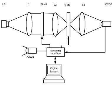
Through CCD1, the input scene is captured and uploaded to SLM1 by the switching interface

while lens L1 collimates the coherent light provided by the light source LS. The image loaded on SLM1

is modulated onto the beam and Fourier transformed by lens L1 while the prior computed matched filter

is loaded on SLM2 through the switching interface.

Switching Interface

Digital System

L1 SLM1 CCD2

LS _{L2 SLM2 L3}

CCD1

Figure 2-1: A Matched Filter based Correlator

Although the matched spatial filter produces the highest signal-to-noise ratio in the image plane

1) It requires a priori fabrication of a complex matched filter used in the Fourier plane.

2) It requires accurate alignment along the optical axis and close positioning between the filter and the

Fourier transform of the input.

3) It is difficult to implement in real time.

4) It requires a second SLM to display phase information, thus an extra cost.

In an effort to improve the spatial filter based correlator, Vander lugt [20] and Cai [21] studied

the effects of misalignment of optical setup, while Montes-Usategui [22] presented an automated

iterative process to correct some of the misalignment that occurs during operations. Davis [23] and

Juvells [24] used divergent lens and photographic teleobjective respectively between the scene and the

filter in an attempt to reduce the correlation setup size.

2.3 J

T

C

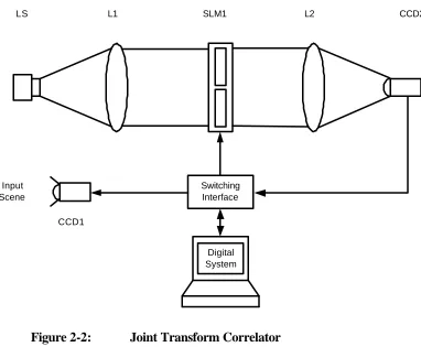
Weaver and Goodman [3] originally proposed the joint transform correlator (JTC) for optically

convolving two functions. This technique has shown remarkable promise for real-time applications like

optical pattern recognition and tracking application. A JTC can be summarized as a two-staged Fourier

transform operation attained on the simple principle of a lens focusing a beam of coherent light that has

been modulated with images [3]. To explain the basic theory of optical correlation, a simplified JTC is

setup up as shown in Figure 2-2. In this approach, light from a coherent source LS is collimated by lens

Switching Interface

Digital System

L1 SLM1 L2 CCD2

LS

CCD1 Input

Scene

Figure 2-2: Joint Transform Correlator

On SLM1, both the input target imaget x y( , )captured using CCD1 and the reference image

( , )

r x y downloaded from the digital system are placed side to side with a separation (

y

0 0

( , ) ( , ) ( , ) (5)

f x y =r x y−y +t x y+y

A physical separation (2 y) between the reference object and the target object is required (as shown in

Figure 2-3) because of the existence of zero-order spectra. This requirement hampers the utilization

efficiency of the input spatial domain and lowers the diffraction efficiency of the correlation peaks. Lens

L2 Fourier transforms the input joint input image f x y( , ) to form

{

}

0 0

( , ) ( , ) ( , )exp[ ] ( , )exp[ ]

( , ) exp[ ( , )]exp[_r ] ( , ) exp[ ( , )]exp[_t ] (6)

F u v f x y T u v jyv R u v jyv

R u v φ u v jy v T u v φ u v jy v

= ℑ = − + −

where R(u,v) and T(u,v) represent the magnitude whileφ_r(u,v)and φ_t(u,v) are the phases for the

reference and target images respectively. The frequency-domain variables are mutually independent and

are represented by uandv.

Figure 2-3: Joint Input Image

The Joint Power Spectrum (JPS) which defines the intensity of the Fourier Transform is

captured by a square law detector CCD2, and is expressed mathematically as

2 ( , ) ( , )

2 2 2 2

( , ) ( , ) 2 ( , ) ( , ) cos[ ( , ) ( , ) 2 ] (7) 0

G u v F u v

R u v T u v R u v T u v φ_r u v φ_t u v vy

=

= + + × − +

To obtain the final correlation outputc(x,y), the JPS is inversely Fourier Transformed as

shown in Figure 2-4, giving the following equation

( , ) ( , ) ( , ) ( , ) ( , )

( , 2 ) ( , 2 ) ( , 2 ) ( , 2 ) (8)

C x y r x y r x y t x y t x y

r x y y t x y y r x y y t x y y

∗ ∗

∗ ∗

= ⊗ + ⊗

where Crr( , )x y :Autocorrelation of the reference image (zero-order),C x ytt( , ): Autocorrelation of the

test image (zero-order), C x y_tr( , −2 )y : Cross correlation of the reference image and the test image located at displacement 2y (first-order), C_rt( ,x y+2 )y : Cross correlation of the reference image and the test image located at displacement 2y (first-order) and ⊗stands for a correlation operation while * denotes the complex conjugates.

Figure 2-4: Correlation Output

As mention earlier, classical JTC is associated with a high zero order peak, which causes

an overlap with the desired cross-correlation whenever there is noise or distortion. In real

implementation, zero order peaks cause strong spurious reflections that over saturates the output

detector [25]. To alleviate these limitations, a binary JTC is used where the joint power spectrum (JPS)

is binarized based on a hard clipping nonlinearity at the Fourier plane to only two values, +1 and -1,

2.4 F

P

I

S

A Fourier plane image subtraction technique [9] helps eliminate the false alarms that are

generated automatically in a JTC when multiple targets or multiple reference objects are present in an

input scene. To implement the technique a modified JPS can be obtained by subtracting both the

input-scene-only power spectrum I u v( , )2 recorded by displaying the input scene at the input plane in the

absence of the reference image and the reference-image-only power spectrum R u v( , )2 recorded by

displaying only the reference image. Since the JPS F u v( , )2 is normally recorded by displaying both

the reference image and the input scene in the input plane SLM, the modified JPS obtained using the

Fourier plane image subtraction technique can be expressed as

[

]

[

]

2 2 2

0 1

0

( , ) ( , ) ( , ) ( , )

2 ( , ) ( , ) cos ( , ) ( , ) 2 2 ( , ) ( , )

cos ( , ) ( , ) 2 (9)

n

i tt r i i

i

r n

P u v F u v T u v R u v

T u v R u v u v u v ux vy vy R u v N u v

u v u v vy

φ φ φ φ = = − − = − − − − + × − −

∑

This equation (9) clearly indicates that the subtraction operation eliminates the false alarms

generated by similar input scene images. It also eliminates the cross correlation terms between other

objects that are present in the input scene. From the above discussion, we see that Fourier plane image

subtraction technique involves multiple processing steps and thus not suitable for real time applications

where processing speed is a key factor. Furthermore, it still requires the use of large SLM to

accommodate the displacement between the images. The technique can be implemented either optically

or electronically.

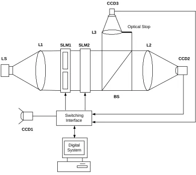
Figure 2-5 illustrates the architecture of a JTC employing Fourier subtraction technique, where

system. Light from light source LS is collimated by lens L1 and passed through SLM1 and SLM2

(phase only SLM), where it is modulated with input information and phase encoded. In the initial

operation, the phase only SLM2 is clear, and light passes without being encoded. Beam splitter BS

splits the beam of light into two: one through L2 and the other through L3. The Fourier transform of the

joint input image is performed by lens L3, captured and downloaded to the digital system by CCD2. An

optical stop is setup up on the vertical beam path to block the transmission of reference image and allow

only the light modulated with test images pass to L3. In the next operation, SLM2 is set as a phase only

SLM representing the negative values while lens L2 performs the inverse Fourier transform which is

captured by CCD1 as the correlation output.

Switching Interface

L1 SLM1 L2

CCD2 LS

Digital System

CCD1

SLM2 L3

CCD3

Optical Stop

BS

2.5 B

JTC

Proposed by Javidi and Kuo, [26] binary JTC is superior to classical JTC in terms of

correlation peak intensity, correlation width, and discrimination sensitivity [25], but is noted to have

lower system processing speed due to the intensive computation required by Fourier plane binarization

process. In this process the JPS is binarized into two values (+1 and -1) based on a hardcliping

nonlinearity before the inverse transformation process. The threshold for binarization is set by making

the histogram of the pixel values of JPS and selecting the median [8].

2 2 1 ( , )

( , ) (10)

1

T if F u v F u v

otherwise

+ ≥

 = ₋



The architecture of the binary JTC is similar to the architecture of the classic JTC shown in

Figure 2-2. The SLM1 is used to display both the input signal and the threshold Fourier transform

interference intensity which is the JPS captured by camera CCD2 and binarized by the digital system.

The correlation output is computed by the lens L2 and read out at CCD2.

2.6 F

-A

JTC

The fringe adjusting technique was proposed by Alam and Karim [8,10] in order to improve

coloration discrimination. In this technique, the JPS is multiplied by a real valued filter referred to as

FAF (fringe adjusted filter) before applying an inverse Fourier transform to yield the correlation output.

( , ) 2

( , )

(11) ( , ) ( , )

FAF u v

B u v H

A u v R u v

=

where A u v( , )and B u v( , )may be constants or functions of v. While A u v( , )is used to overcome the

pole and suppress noise, B u v( , )is used to control the optical gain. By multiplying, the JPS With the

FAF then the modified JPS mentioned earlier is obtained

[

]

( , ) ( , ) ( , ) ( , ) cos ( , ) ( , ) 2

( , ) (12)

( , ) ( , )

FAF

r r

G u v F u v H

R u v T u v R u v T u v u v u v vy

B u v

A u v R u v

φ φ

= ×

+ + − +

=

+

when B u v( , )=1 and R u v( , )2 ? A v( ) then equation (14) can be simplified as

2

( , ) ( , ) (13)

FAF u v

H ≈ R u v −

and the modified JPS is given by the approximation of equation (12)

[

]

( , ) 2 2cos _r( , ) _r( , ) 2 (14)

G u v = + φ u v −φ u v + vy

Although FJTC suffers from false alarms in the presence of multi-target, it does not require high

computations as binary JTC or produce high order harmonics as in a classical JTC [3]. To illustrate the

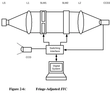
fridge adjusting techniques, the opto-electronic system is setup as in

Figure 2-6. In this fringe-adjusted architecture, the SLM2 is initial set to a transparent mode to allow

CCD2 to capture the JPS. On the next operation, SLM2 is loaded with the fridge-adjusted filter from

the digital system. Lens 2 performs inverse Fourier transform of product of input image and the

Switching Interface

Digital System

L1 SLM1 L2 CCD2

LS SLM2

CCD

Figure 2-6: Fringe-Adjusted JTC

2.7 P

-E

JTC

When the input scene consists of multiple images, the JPS is cluttered with correlation and

autocorrelation peaks that distort each other and are hard to distinguish from one another. The Fourier

plane image subtraction technique mentioned earlier is one of the method used eliminate the zero-order

peak. The phase encoding technique is simpler method that can be employed to achieve the same

effects without the need for digital computation and extra processing steps. The phase mask in this

technique can be represented by [8, 27]

[

]

( , )u v exp jψ( , )u v (15)

Φ =

0 1

( , ) ( , ) ( , ) ( , ) (16)

N

i i i

i

f x y r x y y t x y y ϕ x y

=

= + +

∑

where ϕi( , )x y is the spatial domain transformation of the phase mask. At the correlation output, the

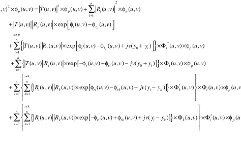
JPS captured is

[

]

[

]

[

]

{

}

[

]

{

}

( , ) ( , ) exp ( , ) exp( ) ( , ) exp ( , ) exp( ) ( , )

( , ) ( , )

( , ) ( , ) exp ( , ) ( , ) ( ) ( , )

( , ) ( , ) e x p ( , ) ( , ) ( )

n

i i ti i

i n

i i n

i t ti i i

i

i t ri i

i

F u v T u v u v juy R u v u v juy u v

T u v R u v

T u v R u v u v u v jv y y u v

T u v R u v u v u v jv y y

φ φ φ φ φ φ φ = = = = + − × = + + × − + + × Φ + − + − +

∑

∑

∑

[

]

{

}

[

]

{

}

( , ) ( , ) exp ( , ) ( , ) ( ) ( , ) ( , )

( , ) ( , ) exp ( , ) ( , ) ( ) ( , ) ( , )

(17) n i i k n n

i k ri rk i k k i

i k

i k n n

i k ri rk i k k i

i k

u v

R u v R u v u v u v jv y y u v u v

R u v R u v u v u v jv y y u v u v

φ φ φ φ = ≠ = = ≠ = = × Φ     + _ × − − − ×Φ _× Φ         +  × − + + − × Φ × Φ    

∑

∑ ∑

∑ ∑

When JPS is multiplied by the same phase maskΦ( , )u v , the cross correlation between the reference image and the test image is preserved while all other peaks are scattered in all directions and

{

}

( , ) ( , ) exp ( , ) ( , )

( , ) ( , ) exp ( , ) ( , ) ( ) ( , ) ( , )

( , ) ( , ) exp ( , ) ( , )

p

p

n

p p i p

i

p t r

n p n

i t t i i p

i

i t ri

F u v u v T u v u v R u v u v

T u v R u v u v u v

T u v R u v u v u v jv y y u v u v

T u v R u v u v u v

φ φ φ φ φ φ φ φ φ φ = ≠ = × = × + ×   + × _ − _   + × _ − + + _ ×Φ × + × − + −

∑

∑

[

]

{

}

[

]

{

}

[

]

{

}

( , ) ( , ) exp ( , ) ( , ) ( ) ( , ) ( , ) ( , )

( , ) ( , ) exp ( , ) ( , ) ( ) ( , ) n

i i p

i i k

n n

i k ri rk i k k i p

i k

i k n

i k ri rk i k k

i k

jv y y u v u v

R u v R u v u v u v jv y y u v u v u v

R u v R u v u v u v jv y y u v

φ φ φ φ φ φ = ≠ = = ≠ = = + × Φ ×     + _ × − − − × Φ _× Φ ×         +  × − + + − ×Φ     

∑

∑ ∑

∑

i u v φp u v

×Φ ×

∑

To avoid affecting the overall speed of the phase encoded JTC, the phase masks are

computed a priori and stored with the reference images in the digital system.

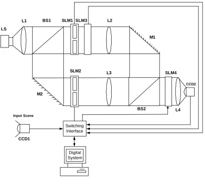
Figure 2-8 shows the architecture of a phase-encoded JTC, which is simple and cost effective

to implement. The laser beam from source LS is split into two beams by beam splitter BS1 after

being collimated by lens L1. At SLM1 the horizontal beam is modulated with input scene image

captured by CCD1and loaded through the digital system switch to the upper part of the SLM3,

which is a phase only SLM that is loaded via digital system with the spatial domain phase mask

from the computer. The mirror M1 steers the Fourier transform of the phase encoded input

scene performed by L2 into BS2. The vertical light from BS1 is steered by mirror M2 into

SLM2, where it is modulated with the reference image that was loaded from the computer to

the lower half of the SLM. BS2 combines the Fourier transform of the reference image

performed by lens L3 and the Fourier transform of the phase-encoded input performed by L2.

The Fourier domain version of the phase mask is downloaded to a phase only SLM4 such that

the combined beam traveling through it is multiplied by the phase mask in Fourier domain. Lens

L4 performs the inverse Fourier transform on the combined beam leaving SLM4. The power

Switching Interface

L1 SLM1 L2

CCD2

LS

Digital System

CCD1

SLM3

BS2 L3

L4 SLM4 M1

M2

SLM2 BS1

Input Scene

3 RANDOM PHASE MASK

This section provides a short overview of the theory and application of Pseudo-random

sequences, focusing mainly on how M-sequences are used to generate two dimensional array

orthogonal phase masks. Pseudo-random sequences are defined as deterministic sequence of integers,

which have been chosen in some methodical manner, but appear to be random [29].

3.1 M-

In creating a phase mask, M-sequence is the preferred Pseudo-random sequence due to ease

of generation. Maximal length sequences (M-sequences) have been utilized widely in numerous modern

communications since first introduced by Zierler in 1967 [30] and their theoretical foundations were

greatly expanded by Golomb [31]. For randomness, the following properties must be satisfied [32]:

• Balance: – the number of ones (high state) in one period must be equal to the number of zeros (low state), or the difference of the number of ones (xn−1) and zeros 1

(xn− −1)should not be more than one.

• Run Property: – defined as a maximal string of consecutive identical symbols (zeros or ones) in the sequence. For M-sequence in a period, half of the runs have a length 1, one quarter have

length 2, one eighth of length 3.

A linear feedback shift register with a generating polynomial g x( ) in which a coefficient arises

from the Galois field [32] can be used generate M-sequence. Finite (Galois) fields are fields with only a

finite number of elements that are closed under operations of addition, subtraction, multiplication, and

division by non-zero elements. These fields exist only when the elements are N

p where P is a prime and

N any positive integer.

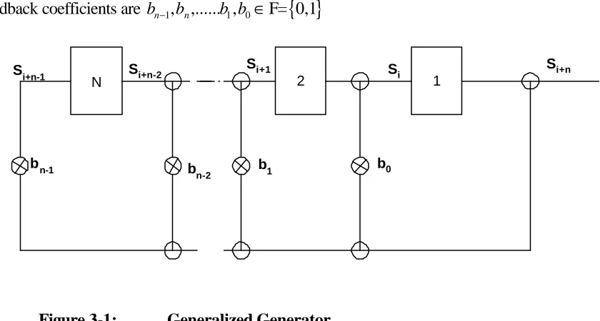
Figure 3-1 is simple set up of shift registers whose contents modified at every step by a binary –

weighted value of the output stage. Considering the initial state of the registers and the feedback

arrangement, the LSFR method generates a sequence {b} that satisfies linear recursion formula.

1

1 i n .... 0 (19)

i n n i

S₊ =b S₋ + − + +b S

where feedback coefficients are b_n−1,b_n,... ,b b_{1 0}∈F= 0,1

{ }

1 2

N

b_{n-1 b}

n-2 b1

b₀

S_i+n-1 S_i+n-2 Si+1 _S

i Si+n

Figure 3-1: Generalized Generator

The succession state of the LFSR form a purely period sequence of period length d ≤2k −1

where k is the order of the shift register sequence. To derive the characteristic polynomial of shift

0

( ) _i i (20)

i

G x b x

∞ =

=

∑

where x is an indeterminate

( )

G x reflects the properties of the sequence {b} and represent its terms in correct order

0 0 0 0 1 1 0 0 ( ) ... (21) k i j i j i j

k

j i j

j i j

j i

k

j j i

j j i

j i

G x a b x

a x b x

a x b x b x b x

∞ − = = ∞ − − = = ∞ − − − − = = = =   = _ + + + _  

∑ ∑

∑ ∑

∑

∑

(

)

1 1 ( ) ... ( ) k j j j j j

G x a x b x₋ − b x₋ − G x

=

=

∑

(

)

1 1

1 ...

( ) (22)

1

k _{j j}

j j

j

k j

j j

a x b x b x

G x a x − − − − = = + + = −

∑

∑

In equation (21) G x( )can be separated into

(

)

1 k

j j= a

∑

1

1 k _j j

j= a x

−

∑

b (values of 0 and 1 equation (21) can be expressed as

1

( ) (23)

1 k k _j j j a G x a x = = −

∑

1

2 1

1 2 1

2 1

1 2 1

( ) 1

1 ...

1 ... (mod2). (24)

k _j j j k k k k k k k k

f x a x

a x a x a x a x

a x a x a x a x

= − − − − = − = − − − − − ≡ + + + + +

∑

If we assume a_kis non-zero (i.e. a_k =1 ) and the characteristic polynomial f x( ) is expressed in th k

degree to be

1

1 1

( ) k _k k ... 1 (25)

For a given initial state

0 1

( ) (26)

( )

i i i

G x b x

f x

∞ =

= =

∑

As earlier stated sequence {b} generated from LSFR is periodic at length d ≤2k −1

Suppose the sequence {b} have a period length of d

1 1

0 1 1 0 1 1

2 1

0 1 1

1 2 3

0 1 1

1

0 1 1

1

( . . . ) ( . . . )

( )

( . . . ) . . .

( . . . )(1 . . .)

( . . . )

(27) (1 ).

d d d

d d

d d

d

d d d d

d d d

d

b b x b x x b b x b x

f x

x b b x b x

b b x b x x x x

b b x b x

x − − − − − − − − − − = + + + + + + + + + + + + = + + + + + + + + + + = ₋

Sincef x( ) is characteristic polynomial it divides by 1 d x

− and the quotient can be expressed as

1

0 1 . . . 1 (28)

d d x x β β β − − + + + then 1

0 1 1

1 2

0 1 1

1 1

0 1 1 0 1 1

0

. . . 1

( ) 1

( . . . )(1 . . . )

( . . . ) ( . . . ) . . .

( ) (29)

d d d

d d d

d

d d d

d d

i i i

x x

f x x

x x x x

x x x x x

G x b x

β β β β β β β β β β β β − − − − − − − − ∞ = + + + = − = + + + + + + = + + + + + + + + = =

∑

This shows that for a sequence {b} with a period length d, the equating coefficients are similar to the

powers of x.

Table 3.1 contain M-sequence feedback sets for LFSR [33].

Shift Register length, n Possible Feedback Taps

2 [2,1]

3 [3,1]

4 [4,1]

5 [5,2], [5,4,3,2], [5,4,2,1]

6 [6,1], [6,5,2,1], [6,5,3,2]

7

[7,1], [7,3], [7,3,2,1], [7,4,3,2], [7,6,4,2], [7,6,3,1],[7,6,5,2],

[7,6,5,4,2,1], [7,5,4,3,2,1]

8

[8,4,3,2], [8,6,5,3], [8,6,5,2], [8,5,3,1], [8,6,5,1],[8,7,6,1],

[8,7,6,5, 2,1], [8,6,4,3,2,1]

Table 3-1: Polynomial Roots

3.2 T

D

A

Two-dimensional arrays can be implemented using the following methods.

• Folding Array: - Mac Williams and Sloane [34] and Green [35] used this method to create a matrix of the same periodic autocorrelation as the M-sequence. To implement a 2D array, a sequence of

length pq is remapped into array of areapqwith p and qbeing co-primes.

based on the concept that all accumulated cyclic shifts between rows separated by distance d are

different (Distinct sums property) [35].

• Product array: – a 2D array is created by multiplying two sequences r and s of lengths p and q element by element. If the two sequences r and s are equal (r=s) then operation can be reduced to a shift-and-add operation. In 1991, Kuo and Rigasi [36] used this method to create

m-arrays, which have found applications in coded aperture imaging, pattern synchronization, code

division and image multiplexing.

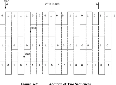
3.2.1 Shift and add property

When an M-sequence is shifted in time and added (modulo 2) to a non-shifted version of the

same sequence, an identical sequence shifted by certain number of bits is the result as shown in Figure

3-2.

(31)

i j k

u + u =u

For 0<i j k, , < −2n 1 and

u

For example:

4

3

111100010011010 101011110001001 010111100010011 u

u u

⊕

0 1 1 1 1 0 0 0 1 0 0 1 1 0 1 0 1 1 1

1 1 0 1 0 1 1 1 1 0 0 0 1 0 0 1 1 0

1 0 1 0 1 1 1 1 0 0 0 1 0 0 1 1 0 1 24_{-1=15 bits}

start

start

start

Figure 3-2: Addition of Two Sequences

A shift

i

(2 1)

(32)

n i i

u =u± −

for 0≤ <i 2n−1

Using the above theory a two dimensional m-array can be constructed from two M-sequence [a] and

[b].where [ ] [ , ...,_{0 1 1}]

a

n

a = a a a ₋ and [ ] [ , ...,_{0 1 1}]

b

n

b = b b b ₋ to form [M] as in equation (33)

0 0 0 1 0 1

1 0 1 1 1 1

1 0 1 1 1 1

. . .

. . .

. . . .

[ ] (33)

. . . .

. . . .

. . .

b

b

a a a b

n

n

n n n n

a b a b a b

a b a b a b

M

a b a b a b

Since every row and column is a modulo-2 addition of an sequence, the m-array consists of

M-sequences and their complement, thus preserving all their properties as shown in Figure 3-3. In addition,

there is more freedom in selecting the size of the array.

For example:

4

3

111100010011010 101011110001001 010111100010011 u

u u

⊕

⊕

1 0 1 0 1 1 1 1 0 0 0 1 0 0 1

1

0

1

0

1

0 0 0 0

1 1 1

0

1 1

0

1 0

1

0

1

0 0 0 0

1 1 1

0

1 1

0

1 0

1

0

1

0 0 0 0

1 1 1

0

1 1

0

1 0

1

0

1

0 0 0 0

1 1 1

0

1 1

0

0 1

0

1

0

1

1 1 1

0 0 0

1

0 0

1

0 1

0

1

0

1

1

1 1

0 0 0

1

0 0

1

0 1

0

1

0

1 1

1

1

0 0 0

1

0 0

1

1 0

1

0

1

0 0 0

0

1 1 1

0

1 1

0

0 1

0

1

0

1 1 1 1

0

0 0

1

0 0

1

0 1

0

1

0

1 1 1 1

0

0

0

1

0 0

1

1 0

1

0

1

0 0 0 0

1 1

1

0

1 1

0

1 0

1

0

1

0 0 0 0

1 1 1

0

1 1

0

0 1

0

1

0

1 1 1 1

0 0 0

1

0

0

1

1 0

1

0

1

0 0 0 0

1 1 1

0

1

1

0

0 1

0

1

0

1 1 1 1

0 0 0

1

0 0

1

3.2.2 Array Auto-Correlation

The cyclic auto correlation

Θ

( , )

( , 0 )

(0, )

(0,0)

1, 0 & 0

, 0

(34)

, 0

, 0

A A i j

A A i b

AA j a

AA a b

for i j

n for i

n for i

n n for i

Θ = ≠ ≠  Θ = − ≠  Θ = − ≠  Θ = ≠ 

By definition, it measures how an array matches a copy of itself as the copy is shifted and mathematical

proven in [36].

3.2.3 Array Cross-Correlation

The cyclic cross correlation Θ_{AA i j}'_{( , )}between two different two-dimensional m-arrays

[ ]

A

and

[ ']

A

'( , ) '( ) '( ) (35)

AA i j aa i bb j

Θ = Θ Θ

where

[ ']

A

[ ']

a

[ ']

b

between the two different arrays.

3.3 R

P

M

A

In this section, we describe a step-by-step procedure to design an optical phase mask. The

steps involves designing an M-sequence from a LFSR and using it to generate a two dimensional

orthogonal array which is converted to phase mask. These steps are summarized in Figure 3-4.

Input: A sequence ai ≡(a a₀i, ₁i,...ai_N−1)

Output: Random Phase Mask

1. Generate M-sequence

a

≡

(

a a

,

,...

a

)

2. Generate shifted sequences

a

≡

(

a a

,

,...

a

)

where i=1,2,...N−1 for N is the length of the sequence code.

3. For 0≤ ≤ −i N 1 choose two sequence codes A and B (

A

≠

B

0 1 1

(

,

,...

)

i i i i

N

a

≡

a a

a

where T represents transpose.

4. Using modulo 2 additions, add bit by bit the two vectors to form a matrix M.

5. create a matrix consisting of

(

N

+ ×

1) (

N

+

1)

padded M matrix.

6. For

M

=

(

m

)

i

= =

j

N

+

1

LFSR

m sequense Shifted

m sequense

Modulo 2 Addition

N X N Array

Random Phase Mask

Conversion

Figure 3-4: Formulation of Random Phase Mask

3.4 C

D

Histograms have been widely used to represent, analyze, and characterize images. They are

easy to compute and represent the approximations of the probability density functions of random

variables whose realization is the particular set of pixel values found in the images. In order to investigate

the effects of varying levels of phase encoding of the phase masks implemented with maximal length

sequence, we first analyze the histograms of images phase encoded with different levels: binary (2),

M-sequence is represented by equationn=mx−1, where m (m = 2, 3, 5) is the level of encoding selected. From the figures below (Figure 3-5, Figure 3-6, Figure 3-7), several observations can be

made about the distribution of the phases in the encoded image. As we increase the number of levels

(m), the peak height of the histograms increase and the curve smoothens. Figure 3-7 (m=5) offers best

results compared to the other two encoding levels (m= 2, 3).This implies that when the reference image

is encoded into more phase mask thus more pixels, it offers better results. In addition, we note that

when identical images are multiplied with different randomized phase masks, their histograms plots are

of Gaussian shape but of different heights.

Figure 3-6: Histogram of ternary encoding (m=3)

Figure 3-7: Histogram of level five encoding (m=5)

Next, we consider the influence of the phase encoding levels on the performance of the phase

encoded JTC. Using the selected three levels (m = 2, 3, 5) to create different phase masks, the

correlation output of the phase encoded JTC binary encoded phase mask. The presence of two peaks

at the correlation output deviates from the expected results. The presence of a conjugate cross

correlation peak in the output plane confirms the inability of binary two phase to disperse all undesired

peaks. From this, we can infer that a phase mask created from a binary

M-sequence is not suitable for encoding images in the JTC system.

Through comparison, level- 5 encoding represented by correlation output in

Figure 3-10 has a better correlation output compared to binary and ternary encoding. The correlation

peaks are distinguished clearly and their intensity height increases as the number of levels were increased

(from 2, 3, and infinity for rand sequence). Figure 3-11 shows the correlation output when phase mask

is created from a random sequences (Matlab rand function was used to create the Pseudo random

sequence).

Figure 3-8: Correlation Outputs for Image created with a Random phase

Figure 3-9: Correlation Outputs for Image created with a Random phase mask (m=3)

Figure 3-10: Correlation Outputs for Image created with a Random phase

4 MULTI-REFERENCE PHASE ENDODED JTC

This section presents an analysis of the multi-reference phase encoded JTC and sheds light on

the implemented multi-reference phase encoded JTC using a phase only SLM. The goal of the section

is to mathematical express the mentioned architectures and compares their results.

Using a multiple reference image in the input joint image to correlate with a single test image in a single

step, Alsamman [37] presented a multiple reference phase encoded JTC that takes advantage of the

massive parallelism of optical systems to increase the processing power of the JTC. In this technique,

reference images are phase encoded using Pseudo-random sequences, hence removing extraneous

peaks from correlation plane as well as improving the spatially efficiency of the JTC system.

In a classical JTC, a minimum SLM size of 2N X 2N is required to correlate two N X N

images. This is because of the displacement (2y₀) required between the reference image and the test

image to avoid zero order term in the correlation output dominating and overshadowing the cross

correlation terms. A displacement of distance(2y₀)at the input plane results in double distance (4y₀

between the cross correlation terms) at output plane. In order to obtain large displacement without

increasing the sizes of the SLM, small images are used which result to a lower discrimination power at

correlation output plane. The use of large SLM size vastly increases the overall cost of the JTC while

increasing the overall system size.

In the multi-reference phase encoding technique, every reference image is multiplied with a

phase mask defined as

[

]

( , )u v exp jψ( , )u v (36)

where ψ( , )u v is a random phase distribution between

−

π

π

The joint input image of multi-reference phase encoded JTC represented by the equation below

consists of a reference image ( , )r x y_i that has been encoded with phase mask ϕ_i( , )x y and displayed

side by side with an input test image.

1

( , ) ( , ) ( , ) ( , ) (37)

N

i i

i

f x y t x y r x y ϕ x y

=

= +

∑

Using light from source LS and collimated by lens L1, the joint input image is displayed on

SLM1 (Figure 4-1). The converging lens L2 is used to obtain the Fourier transform of joint input image

and the JPS captured by the CCD device and routed to SLM1 through the digital interface as shown on

Figure 4-1

[

]

[

]

[

]

{

}

[

]

{

}

( , ) ( , ) exp ( , ) ( , )exp ( , ) ( , )

( , ) ( , )

( , ) ( , ) exp ( , ) ( , ) ( , )

( , ) ( , ) exp ( , ) ( , ) ( , )

( , ) ( , ) exp ( , )

n

i i ti

i

n

i i n

i t ti i

i n

i t ri i

i

i k ri

F u v T u v u v R u v u v u v

T u v R u v

T u v R u v u v u v u v

T u v R u v u v u v u v

R u v R u v u v

φ φ φ φ φ φ φ φ = = = = = + × = + + × − ×Φ + − + ×Φ + ×

∑

∑

∑

∑

[

]

{

}

[

]

{

}

( , ) ( , ) exp ( , ) ( , ) ( , ) ( , )

(38)

i k n n

rk k i

i k

i k n n

i k ri rk k i

i k

u v u v u v

R u v R u v u v u v u v u v

To obtain results for a particular reference image, its corresponding phase mask is displayed on

SLM2 and correlated through lens L2. The same process can be achieved by multiplying the JPS

digitally with the phase mask

Switching Interface

Digital System

L1 SLM1 L2 CCD

LS SLM2

Phase Only

Figure 4-1: Multi-Reference Phase Encoded JTC

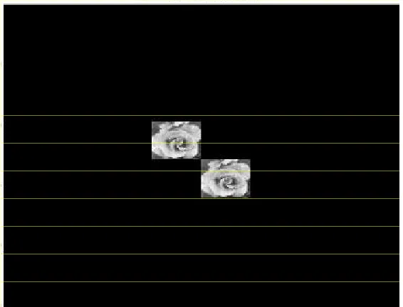
Figure 4-2 shows the joint input image with two reference image of size 256 X 256 pixels

phase encoded with a phase mask created from five level maximal length sequences

(M-sequences). The shift and add method described in chapter three was used to create an m-array

which was translated into a phase mask of size 256 X 256. In Figure 4-2 below only the test image can

clearly be identified, as the phase encoded reference images pixels are scattered by the phase mask in

all directions and appear as noise. Figure 4-3 represents the correlation output achieved using a

Figure 4-2: Joint Input Image

4.1 M

-R

P

E

JTC U

P

SLM O

In this thesis, we further improve the performance of the multi-reference phase encoded JTC

by converting both the reference and target image into phase information before applying operations

similar to multi-reference phase encoded JTC discussed earlier. From the previous phase encoding

technique, we have seen that Fourier plane image subtraction technique results are attained using a

random phase mask generated from two-dimensional M-sequence array. The advantage of this method

is that the same effects are achieved with less digital computation and without extra processing steps

[37]. Phase encoding technique has also been successful used in the field of information security as in

optical authenticity verification [38] and in storing encrypted information holographical [39].

In the initial stage, all images are encoded with a phase expression forming a phase only

representation. Target image and reference image are converted into the following expressions

( , ) exp[ { ( , )}] (39)

pt x y = jA t x y

( , ) exp[ { ( , )}] (40)

pr p q = jA r x y

where A is phase depth (2 )π

The technique of transforming intensity images into phase function has been previous used in pattern

recognition pattern [38,39]. The joint input image used in this system consists of target image placed

side by with multiplexed references images as expressed below equation and shown in Figure 4-4:

1

( , ) ( , ) ( , ) ( , ) (41)

N

i i

i

pf x y pt x y pr x y ϕ x y

=

= +

∑

where ϕ_i( , )x y is the spatial domain transformation of the phase mask that is expressed as

[

]

( , )u v exp jψ( , )u v (36)

Φ =

Different shifts of M-sequence are used to create orthogonal phase masks that are used multiplied with

every reference image in Fourier domain.

Figure 4-4: Joint Input Image

The JPS collected by CCD at the correlation output can be expressed as

[

]

[

]

[

]

{

}

[

]

{

}

( , ) ( , ) exp ( , ) ( , ) exp ( , ) ( , )

( , ) ( , )

( , ) ( , ) exp ( , ) ( , ) ( , )

( , ) ( , )exp ( , ) ( , ) ( , )

( , ) ( , ) n

i i ti

i

n

i i n

i t ti i

i n

i t ri i

i

i k

PF u v PT u v u v PR u v u v u v

PT u v PR u v

PT u v PR u v u v u v u v

PT u v PR u v u v u v u v

PR u v PR u v

φ φ φ φ φ φ φ = = = = = + × = + + × − ×Φ + − + ×Φ + ×

∑

∑

∑

∑

[

]

{

}

[

]

{

}

exp ( , ) ( , ) ( , ) ( , )

( , ) ( , ) exp ( , ) ( , ) ( , ) ( , ) (42) i k

n n

ri rk k i

i k

i k n n

i k ri rk k i

i k

u v u v u v u v

PR u v PR u v u v u v u v u v