University of New Orleans University of New Orleans
ScholarWorks@UNO
ScholarWorks@UNO
University of New Orleans Theses and
Dissertations Dissertations and Theses
8-6-2009
An Analysis of netCDF-FastBit Integration and Primitive
An Analysis of netCDF-FastBit Integration and Primitive
Spatial-Temporal Operations
Temporal Operations
David Marks
University of New Orleans
Follow this and additional works at: https://scholarworks.uno.edu/td
Recommended Citation Recommended Citation
Marks, David, "An Analysis of netCDF-FastBit Integration and Primitive Spatial-Temporal Operations" (2009). University of New Orleans Theses and Dissertations. 984.
https://scholarworks.uno.edu/td/984
This Thesis is protected by copyright and/or related rights. It has been brought to you by ScholarWorks@UNO with permission from the rights-holder(s). You are free to use this Thesis in any way that is permitted by the copyright and related rights legislation that applies to your use. For other uses you need to obtain permission from the rights-holder(s) directly, unless additional rights are indicated by a Creative Commons license in the record and/or on the work itself.
An Analysis of netCDF-FastBit Integration and Primitive Spatial-Temporal Operations
A Thesis
Submitted to the Graduate Faculty of the University of New Orleans
in partial fulfillment of the requirements for the degree of
Master of Science in
Computer Science
by
David Marks
B.S University of New Orleans, 2005
Table of Contents
Table of Figures... iii
Table of Tables... iv
Abstract... v
Chapter 1: Introduction... 1
1.1 Summary... 1
1.2 Defining Terms... 3
1.2.1 What is netCDF?... 3
1.2.2 What is Bitmap Indexing?... 8
1.2.3 What is FastBit?... 14
1.2.4 What is ncks?... 16
Chapter 2: Proposed Architecture... 18
2.1 System Overview... 18
2.2 Proposed GUI... 20
Chapter 3: FastBit Indexing and netCDF Integration... 25
3.1 Method Used... 25
3.2 Results Obtained... 27
Chapter 4: Implementation and Viewing of Spatio-Temporal Queries... 29
4.1 Temporal Operations... 29
4.2 Spatial Operations... 30
4.3 Proximity Operations... 32
4.4 Statistical Operations... 39
4.5 Visualization... 41
Chapter 5: Conclusions and Future Work... 44
5.1 Future Work... 44
5.2 Conclusions... 47
References... 49
Table of Figures
Figure 1: System Flowchart... 18
Figure 2: The Index Manager and Binning Options Tab... 21
Figure 3: The Encoding Options Tab... 22
Figure 4: The Compression Options Tab... 23
Figure 5: The Query Manager Screen... 24
Figure 6: An Example Bounding Box Describing 500 Meters... 36
Figure 7: A Still Frame From a 2D Animation of Water Temperature... 42
Table of Tables
Table 1: Sample Queries and their Respective Runtime and Speedups... 28
Table 2: Speedup with and without Bounding Box Filter, ~8.75 Million Points... 37
Abstract
A process allowing for the intuitive use of SQL queries on dense
multidimensional data stored in Network Common Data Format (netCDF) files is
developed using advanced bitmap indexing provided by the FastBit bitmap indexing
tool. A method for netCDF data extraction and FastBit index creation is presented and
a geospatial Range and pseudo-KNN search based on the haversine function is
implemented via SQL. A two step filtering algorithm is shown to greatly enhance the
speed of these geospatial queries, allowing for extremely efficient processing of the
netCDF data in bitmap indexed form.
Chapter 1: Introduction
1.1 Summary
Over the past several decades, scientific advances have led to larger and larger
amounts of data becoming available for scientific analysis and study in nearly every
field. What might have once been considered a staggering amount of data is now
often simply dwarfed by the reams of information gathered on a daily basis via
numerous highly advanced sensors throughout the world. Faced with somehow storing
this vast quantity of raw scientific data, researchers found that many of the more
standard database options available were unsuitable for the style of data they
possessed. Thus, a proliferation of scientific data formats have been introduced,
many written by the researchers themselves, aimed at somehow storing their data in
a compact way. Unfortunately, while ever more advanced devices and processes have
allowed for this continuously increasing level of data to be stored efficiently, the
ability to analyze and access this data in an easy and reasonable manner has not kept
similar pace. These scientific data formats, designed with scientific data in mind,
manage to provide compact storage of extremely large amounts of information and a
basic format and structure for their contents. However, the retrieval and access of
the data contained within is often far more complicated, with few ways to easily
extract the data stored within these formats, especially not in a manner familiar to
any modern database users.
One of the main hurdles in utilizing an industry standard database solution involves
classically assumed within current database research. Scientific data is often
extremely multidimensional in nature, with no field suitable for acting as a primary
key. Further, there is rarely even a unique combination of fields which can act as a
primary key; a unique identifier for a data point may often be formed in numerous
different ways, or may simply consist of every field utilized together. These features
present large hurdles with the most commonly utilized indexing methods. However
these features, taken in conjunction with scientific data's generally static nature,
make an uncommon indexing method, bitmap indexing, particularly feasible.
Bitmap indexing suffers from several limitations which generally prevent it from being
used with regular data. Perhaps the largest of these problems is bitmap indexing’s
inefficiency in updating or deleting any of the data records once they have been
indexed. The scientific data files being discussed here, however, are generally static
in nature, often being written once as the product of a multitude of sensors over a
period of time and are otherwise unchanged after creation. Another issue facing
bitmap indexing, the cardinality of the data to be indexed, poses more of a problem
when utilizing scientific data. As discussed within the term definitions of bitmap
indexing and FastBit, however, advances within the field of bitmap indexing have
developed many compression algorithms aimed at overcoming this limitation.
As such, the generation of indexes to these scientific data formats utilizing bitmap
indexing techniques is proposed. The use of these indexes will allow for rapid,
efficient data access within the files in question in a format and method more
project to utilize the FastBit bitmap indexing suite of tools with netCDF files
containing oceanic data are provided. For a one time cost of 25 minutes a reusable
bitmap index was created that is capable of answering equality searches over the
dataset in 1 second, a 1200x speedup compared to the 20 minutes required to read
the entire file. Further, a range query returning all points within a specified distance
of a point is implemented via SQL and tested utilizing the generated bitmap index. A
two step filter is proposed and implemented, resulting in a large speedup in the range
query over a large number of points.
1.2 Defining Terms
The work within this project relies upon several concepts and applications that
have come before so an explanation of what and where each of these pieces are is
provided in this section. Further, a short history of each term is provided to provide
context on the intent and purpose of the idea originally.
1.2.1 What is netCDF?
A shortened version of its full name, netCDF stands for Network Common Data
Form. Initially developed in the early half of 1988 by the National Center for
Atmospheric Research, it was modeled in the beginning after NASA's CDF (Common
Data Format)[18][16]. Originally very close to its conceptual roots, netCDF at first
mostly provided an additional level of machine independence to CDF which was
limited at the time to VAX/VMS environments. Since then, however, both projects
have continued to grow and mature and while still quite similar, now possess many
version 3.0 following shortly in June of 1997. The version used for this project is
netCDF version 4.0, released June of 2008.
Throughout all of that time, netCDF has remained a cross language, freely
distributed, machine independent set of tools and libraries that, along with the
netCDF format itself, allow for the creation, access, and sharing of scientific data.
Implementations of netCDF can be found in C, FORTRAN, C++, Java, Python, and many
other languages. NetCDF is utilized at numerous government and commercial
ventures, not only throughout the United States of America, but throughout the world
itself.
All netCDF data should conform to six principals for netCDF data, possessing the
qualities of self-description, portability, scalability, appendability, sharability, and
archivability. That is, netCDF data should include details as to what information it
contains and be accessible by computers with disparate methods for storing integers,
characters, and floating points. It should efficiently allow access to small subsets of
its data and be accepting of the addition of new data without needing to copy the
dataset or redefine its structure. Finally, netCDF data should be able to support one
writer and multiple readers concurrently and always retain backwards compatibility
with previous versions of netCDF.
At its heart, netCDF is an interface to a library of data access functions designed to
items all with the same data type. A header stands at the beginning of every netCDF
file, containing information regarding the names, types, and characteristics of the
dimensions, attributes, and variables found within the file. This dense structure
serves to help keep netCDF files compact, however if any changes to the file are later
made that must be reflected in the header the entire file may need to be moved to
account for the larger (or smaller) header. Thus common netCDF practices
recommend that all of the dimensions, attributes, and variables be created before
any actual data is written to hopefully avoid a necessitated painful movement of
data. Following the header is the data portion of the netCDF file, consisting of a
mixture of fixed and variable size pieces corresponding to variables possessing no
unlimited length dimensions and variables possessing unlimited length dimensions,
respectively. The header possesses offsets from the start of the data portion to each
of the variables, to enable rapid retrieval of their constituent values.
A netCDF dimension is used as a building block for netCDF variables. In netCDF
dimensions have both a name and a length. The length of a dimension is either an
arbitrary positive integer or unlimited (earlier versions of netCDF were limited to only
one unlimited dimension per document, netCDF 4 allows for any number of unlimited
length dimensions). An unlimited length dimension can continue to grow to any length
without limit and could be analogized to the record ID field in conventional record
oriented file systems. Dimensions can represent a real physical dimension such as
time or height or they can describe more abstract qualities like a sensor's
dimensions, latitude, longitude, height, and time. The first three dimensions
(latitude, longitude, and height) would possess lengths describing the limits of the
physical area from which data has been gathered. If data was gathered at three
separate heights, for example, the length of the height dimension would be three.
The time dimension would possess an unlimited length, indicating that data could
continuously be added to whatever variable is constructed using the time dimension
as the values being observed changed over time.
A variable is the basic unit of named data in a netCDF dataset and they store the bulk
of the data found in netCDF datasets. Variables represent arrays of values of the same
type with scalar values treated as zero dimension arrays. Each variable possesses a
name, data type, and shape as described by the dimensions specified at the variables
creation. A variable can also possess any number of attributes which may be added,
removed, or changed even after a variable has been created. Common convention
suggests a unidimensional variable be created for each of the dimensions within a
netCDF file. These coordinate variables hold information pertaining to the actual
values found along a dimensions axis; utilizing our example from before, a time
coordinate variable would hold the actual time values along which each data sample
was gathered while the height coordinate variable would contain the three heights
from which data readings were taken. A demonstration of a non-coordinate variable
could be any of the taken data readings, varying over the four dimensions depending
on both where and when each specific reading was taken, as long as the data type for
An attribute contains metadata, generally about a specific variable. Some attributes
instead contain global pieces of metadata, information that describes the entire file
itself. Attributes also possess both lengths and data types, although they are far more
versatile than the dimensions and variables. Attributes can be deleted or altered in
data type, length, or value after creation, properties not shared by either dimensions
or variables. Also attributes can be created and added long after a netCDF dataset is
first defined, although this poses the same risk as altering the header after creation in
some cases; the entire file may need to be moved to account for any additional
attributes added post definition. Looking back to our example, each of the five
variables, four coordinate and one non-coordinate, would possess a unit’s attribute
that describes the physical property which the numeric integer values represent.
Other possible examples would be attributes describing the maximum or minimum
allowable values within a variable, or an offset that applies to all of the values
contained by the variable.
In order to comply with the netCDF principal of scalability it is possible to retrieve
small subsets of data from netCDF files without having to read through the data that
physically precedes it. Using the offsets included in the header it is possible to
retrieve individual values from inside any of the variables within the netCDF file
utilizing an index number for where along the variable's dimensions the desired value
lies. There are further methods designed to provide for accessing larger chunks of a
is that in all cases, access to the netCDF data is defined utilizing the concept of the
dimensions over which the variables are defined. Returning once more to our
example, if the latitude, longitude, height, and time of the measurement you desire
are known to you, netCDF already features built in functions that will provide you
easy and efficient access to this information. Instead, however, if you wish to know
the latitude, longitude, height, and time when the measurement taken was a
particular value or fell within the particular range then you would be forced to read
through the entire variable in question comparing each value found by hand to your
value or range of interest. For a file of large size this procedure can take an
unreasonable amount of time creating a need for a better solution.
1.2.2 What is Bitmap Indexing?
Bitmap Indexing, a specialized form of data indexing, has its roots within a
paper published in 1985, "Bit Transposed Files", by H. K. T. Wong, H. Liu, F. Olken, D.
Rotem, Linda Wong. Establishing two of bitmap indexing's distinguishing features, the
paper proposed both the storage of the index's information utilizing bit vectors and
the corresponding use of bitwise logical operations to answer queries[5]. Proposed as a
possible solution to the inherent difficulty in creating a data index on scientific or
statistical data this idea was seen again two years later in 1987 inside a paper titled
"Model 204 Architecture and Performance" by P. O'Neil which presented a full
After these initial developments, however, bitmap indexing came to be seen mostly
as a useful tool for the creation of low space and high efficiency indexes when dealing
with low cardinality data, data with a very small set of possible distinct values. A
classic example of this type of data is gender in the context of exceptionally large
databases containing information on large numbers of people. While the number of
records could be quite high only one of two values would ever be needed meaning two
bit arrays, one representing males and one representing females, could contain a data
representation of the entirety of the gender dataset. Because of the low
computational needs for bitwise logical operations, queries asked utilizing this
arrangement are able to be answered in an extremely efficient manner. This view
developed in response to the recognition of bitmap indexing's "Curse of Cardinality".
Since basic bitmap indexing creates one bitmap for every distinct value found within
the data the number of bitmaps, and thus the size of the entire bitmap index, can
grow to a very large number in the event that the data possesses high cardinality. As
the total size of the bitmap index increases the query time suffers as larger and larger
amounts of data are needed to be scanned before any query can be answered. It does
not require an extraordinarily high level of cardinality before bitmap indexing
becomes a sub par choice of indexing methods creating both larger indexes and
providing slower responses to queries.
Another limitation found to be problematic when utilizing bitmap indexing involves
bitmap indexing's difficulty with dynamic data. Because each distinct value is
bitmap for every distinct value by one to represent the new record in the case that
the new record's value was already present. In the case that a new record's value was
not present, a new bit array representing the entire value requires construction. The
updating, and to a lesser extent the deletion, of records faces similar performance
costs. Oracle, the producer of the highly popular eponymous database, introduced
bitmap indexes into their product in 1997 with version 7.3.4. The limitations
mentioned above featured largely within their advice to their customers, however,
suggesting bitmap indexing be used only in certain limited circumstances, namely
when the data was of low cardinality and dynamism and even then only if other
columns within the data possessed the same qualities so that they could be joined
together using efficient bitwise logical operations.
While bitmap indexing's difficulty in handling dynamic data still proves problematic
today, the scientific data addressed within this paper is mostly static in nature as
described previously. Thus the "Curse of Cardinality" is by far a more serious problem
in utilizing bitmap indexing solutions with the intended data. Three different
strategies are utilized to minimize this particular inherent weakness within bitmap
indexing. The first strategy, compression, is a relatively simple concept that is likely
familiar to many computer scientists. Bitmaps are a highly compressible type of data
and can be compressed down to small sizes even using simple compression routines.
Indeed, by utilizing very simple compression routines such as run-length encoding the
size of bitmap indexes can be compressed smaller than many other indexing options.
properly compressed bitmap index will often be roughly the size of an equivalent
B-Tree[11]. The small size of compressed bitmap indexes lowers both the space needed
to store them and also the amount of processing needed to access them from disk. For
some compression algorithms the resulting compressed bitmaps do not even require
decompression before they can answer queries allowing for their direct utilization in
logical operations while still in their compressed form.[2]
Encoding is another regularly acknowledged strategy for increasing the performance
of bitmap indexes. Instead of creating one bitmap index for each distinct value of the
indexed attribute, an encoding scheme is used to reduce the number of bitmaps
needed to hold the entire index. An easy to understand example would be binary
encoding where instead of creating X bit arrays for the X distinct values of the
indexed attribute, log2(X) bit arrays are created instead and the binary value of all of
a row's bits read together indicates the enumerated value it holds. Thus if an
attribute had ten distinct values four bitmaps could be employed using binary
encoding to describe the value held by each data point. The downside of this
approach, however, is the need to read all four bitmaps to properly answer queries
which could be solved by reading only one bitmap using the more general basic
bitmap encoding. For example, if a query simply requested all data points that
possessed a given value the basic bitmap encoding could examine the single bit array
representing that value and answer the query completely, whereas an index utilizing
binary encoding would need to examine all of the bitmaps in order to determine
encodings generally represent compromises between the space required to actually
store the bitmap indexes and the speed in which they can answer queries. This idea
obscures an even more general principle regarding different encoding schemes,
however. What the various bitmap indexing encoding schemes truly allow is for the
bitmap index's creator to customize the bitmap index for the types of queries it will
predominantly be asked. Different encoding schemes exist for optimizing a bitmap
index to answer equality or range queries, for example, and knowledge of the type of
queries a given bitmap index will predominantly be asked allows for the choice of an
encoding that will best serve those queries.[1]
The third strategy utilized is the concept of binning. A seemingly simple strategy,
binning merely suggests a bitmap index creator dealing with a high cardinality
attribute utilize each bitmap not as an individual value, but as a range of values. In
this way, a binned bitmap index can quickly and efficiently exclude those data points
that lie within bins that are certainly not within the requested set by comparing the
range the bin encodes for against the requested values. If no requested value falls
within the range of the bin no data point within the bin should be returned. Likewise,
those data points which most certainly are within the requested set can also be
swiftly selected by returning all data points within a bin whose range is completely
contained within the requested values. Any bins left over constitute edge bins, whose
set of values within the bit overlaps, but does not equal or contain, the set of
requested values. For example, if a bitmap index was created with five bins
query is submitted asking for those data points whose values are less than 35 but
greater than 7, then the last bin, [41 - 50], can be instantly eliminated. Bins [11 - 20]
and [21 - 30] can be instantly returned, as every data point within them falls inside of
the desired range of values. Bins [1 - 10] and [31 - 40] would constitute the edge bins
in this case and would now need a candidate check, an examination of each data
point individually to determine which ones fall inside of the desired value and which
do not. Just as there are many compression and encoding strategies, so to are there
many approaches to binning. The most basic binning approach merely consists of
equal width bins that evenly divide up the range of values for the indexed attribute.
This simple approach, however, ignores the reality of most real world data and often
results in misshapen bins due to naturally occurring clusters of values within the
indexed attribute's range. More advanced approaches take the nature of the indexed
data into account and attempt to produce equally weighted bins throughout the data
or instead consider the work intended for the index and purposefully position bins to
ensure likely edge bins are smaller than the remainder of the index. One particularly
powerful binning strategy goes so far as to propose an additional data structure used
to increase the candidate check's efficiency. Candidate checks are normally the
bottleneck within a binned bitmap index, often due to having to randomly access all
of the data points within a bin and check them individually. Order-preserving
Bin-based Clustering, however, proposes the use of clusters of the data points within each
bin stored together so that any needed candidate check within a multi-valued bin will
proceed at a much faster pace than usual[12]. Using order-preserving bin-based
binning, trading away some of the spatial savings realized by utilizing the binning
strategy for an increase in query response times. While deciding on how many bins to
use remains a difficult problem to resolve utilizing order-preserving bin-based
clustering has been shown to break the "Curse of Cardinality" for bitmap indexes.
1.2.3 What is FastBit?
FastBit[13][9], developed by the Scientific Data management group at the
Lawrence Berkeley National Laboratory, is an open source free bitmap indexing
toolkit. FastBit is highly developed and utilizes many advanced bitmap indexing
algorithms not only for querying of the indexed data itself but also for efficiently and
optimally compressing, encoding, and binning the bitmaps generated. Intended for
use with complex high cardinality static scientific datasets, FastBit was introduced in
2007. Since then it has continued to be refined and expanded upon and is currently in
use within many applications which deal with complex high dimensional scientific
data.
For compression purposes FastBit utilizes an award winning patented bitmap indexing
compression algorithm known as WAH, or Word Aligned Hybrid. Compression routines
seek to lower the I/O costs of loading the on-disk bitmap indexes into memory for
processing, decreasing their size and allowing them to load faster. For many
compressed bitmap indexes, however, the majority of the time utilized to answer
queries was spent within the CPU performing logical operations. Based on this
realization WAH compression was designed to optimize its usage within the CPU by
the first bit of every word is used to distinguish the word as either a literal word or a
fill word. For literal words, the remaining thirty-one bits (assuming thirty-two bit
words) contains the uncompressed data from the bitmap indexes. Fill words on the
other hand contain a fill bit which indicates what repeating value the fill word is
compressing followed by a count of the number of literal words worth (thirty-one bits,
again assuming thirty-two bit words) of fill bits the fill word represents. In analysis
this approach has been proven optimal[7] as the query response time is proportional to
the number of hits generated by the query while the compression rate achieved still
leaves the compressed bitmaps smaller than a comparable B-Tree. In those rare cases
where a user wishes to leave some or all of their bitmap indexes uncompressed
FastBit also allows for the storage of uncompressed bitmaps based either on their
density or compression ratio.
By default FastBit does not employ any encoding techniques within its bitmap
indexes, instead simply utilizing the basic bitmap index equality encoding scheme
consisting of one bitmap per indexed value. FastBit possesses the ability to use two
other types of encoding, however, range and interval encoding. Range encoding
utilizes the same number of bitmaps as the standard equality encoding but is
optimized for queries requesting a range of values. Interval encoding on the other
hand decreases the number of created bitmaps. As discussed earlier this decreases
the storage space required to hold the index but increases the time needed to query
For binning FastBit offers the same level of flexibility presented with encoding. A user
can choose to create any given number of bins of almost equal weight or at
designated boundary lines. To designate bin boundaries a desired precision or formula
can be given or a direct list of boundaries to utilize. FastBit even allows for the use of
order-preserving bin-based clustering as discussed earlier, creating a set of files
containing the reordered values and storing them with the generated bitmap indexes.
In order to load data within FastBit a user can simply identify a file of comma
separated values along with any options they wish to utilize in the indexes
construction through a command-line interface and FastBit will generate the indexes
automatically. FastBit’s command-line interface also allows for the querying of the
generated bitmaps using a subset of the SQL syntax. This allows queries to be written
in the same format used in many other database applications and thus provides an
easy to use interface which the majority of users will already be familiar with. The
output produced via FastBit can be written to a file as a set of comma separated
values or simply output to the screen. Overall FastBit presents an efficient
implementation of bitmap indexing algorithms, allowing for the indexing and querying
of high dimensional static scientific data.
1.2.4 What is ncks?
Ncks, short for netCDF Kitchen Sink, is a tool included within the open source
nco suite of operators. Released as an open source project in March of 2000 nco, or
the netCDF Operators, was begun by Charlie Zender, an Associate Professor of the
analysis, manipulation, and transformation of netCDF documents, the nco project
contains several different applications that offer a large degree of functionality to
base netCDF files.[15]
As suggested by the name “Kitchen Sink”, the ncks tool itself contains a number of
disparate functions primarily aimed at converting netCDF documents into different
formats, predominantly either ASCII text or flat binary. While such functionality is
simple in concept, in implementation it is far different with the difficulty arising
largely due to netCDF document’s inherent complexity.
Within ncks a user is provided with options for the retrieval of all variables specified,
all variables not specified, or simply all variables in the dataset. Further options allow
for the extraction of any associated coordinate variables along with numerous choices
regarding the formatting of the output. The name and index location for each variable
can be provided along with the value at that data point, or instead output can simply
consist of a labelless collection of values. Metadata can be preserved if desired, or
the values within any unit attributes can be included within the output. Obviously the
transformed output produced through ncks lacks the highly compressed data format
found in netCDF. As such, any meaningful extraction of data using ncks will result in
an ever larger file, although the precise increase in space will vary depending on the
Chapter 2: Proposed Architecture
2.1 System Overview
Often, the first step in the design of a complex system is the construction of a
detailed schema to help visualize the actions taken by the system when in use. For
the use of bitmap indexes with high dimensional scientific data stored in netCDF files
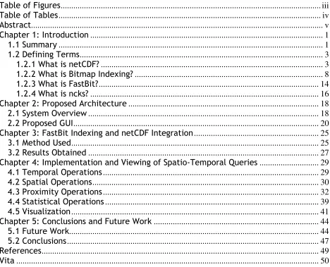
the architecture as depicted in Figure 1 is proposed.
Figure 1: System Flowchart
A Bitmap Index Manager is proposed to build and maintain a bitmap indexes
multiple file bitmap indexing for netCDF scientific data. Further, the netCDF files may
be accessed either locally or across a network. The Metadata Repository will hold any
relevant metadata found within the netCDF file’s header. This metadata will aid in
maintaining organization when several bitmap indexes are used, as well as providing a
boost to query speed by screening out queries from which no point (or perhaps all
points) meets the desired criteria. Further, the metadata will be utilized in any
visualization of a query’s results by providing details such as the extent of the
measured area. The Query Processor’s role is to transform the user submitted high
level queries into sequences of bitwise logical operations executed in the reduced
search space generated using the Metadata Repository. This architecture allows for
the recognition and retrieval of the specific records desired by the user. Compared to
reading through the entire file, this design should result in a substantial speed up.
The Query Manager will seek to optimize the processing of a number of primitive
operations which form the basis of high level queries. Recent studies[6] on the query
processing of mesh data (such as data stored in netCDF files) identify four classes of
primitive operations:
Temporal Operations: query a mesh during a time interval or time point.
Spatial Operations: locate a mesh region of interest
Similarity/Proximity Operations: determine region(s) that are similar to a
given region using a particular distance metric function. The most common examples
Statistical Operations: aggregate per group for a given region. The aggregation
may involve spatial, temporal or field variables.
The details of how our proposed netCDF enabled FastBit handles each of these classes
of operations are presented in chapter 4.
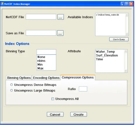
2.2 Proposed GUI
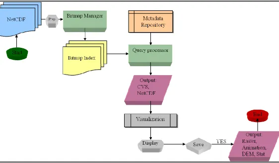
To utilize this proposed architecture a GUI has been designed with the
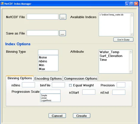
collaboration of Fareed Qaddoura. Figure 2 depicts the Index Manager screen of this
GUI. A user can either browse to a specific netCDF file or enter a URL identifying one.
Any preexistent bitmap indexes having already been created for the netCDF file will
be displayed and can be selected and used with a query right away via the “Use In
Query” button. If no bitmap indexes already exist for this file, or if none of the
indexes available are appropriate for the desired query, a new index can instead be
created using the many index options provided through the “Index Options” section
occupying the bottom half of the screen. As can be seen in Figures 2, 3, and 4, all of
the various bitmap index creation options exposed through FastBit are allowed. When
choosing to create a new index, the variables to be indexed can be selected from the
Figure 4: The Compression Options Tab
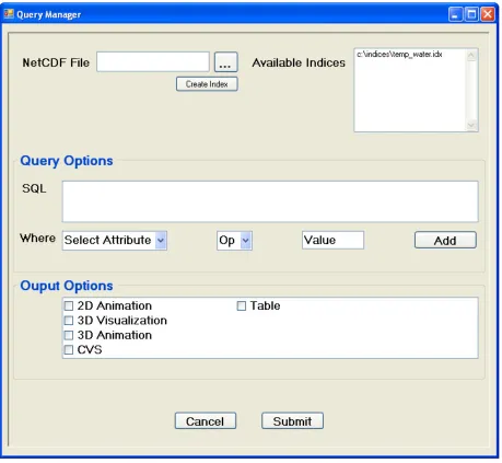
Once an appropriate bitmap index is either selected or created, the Query Manager
screen of the GUI can be used to submit a desired query by the user either by typing
the query directly into the SQL box or by using the drop down Where boxes to create
and add Where clauses, as seen in Figure 5. Further, a number of different output
formats are offered through the Query Manager screen with options ranging from pure
This arrangement leverages FastBit’s many abilities within the proposed architecture
to minimize the learning curve for any new users. Further, the user interface allows a
user to easily see all of the possible options within the proposed architecture, possibly
Chapter 3: FastBit Indexing and netCDF Integration
3.1 Method Used
As mentioned previously, by default FastBit is only able to interpret one type of
input, a file of comma separated values. While the comma separated value reader
utilized by FastBit is tolerant of irregularities within the data, there is no capacity for
interpreting anything similar to netCDF data. In order to load the data stored within a
netCDF file into FastBit, one would need to first convert the data into comma
separated value format. Luckily, several utilities are already existent for the
conversion of netCDF data to comma separated value format, one of which, ncdump,
comes packaged with netCDF itself. However, the concept of comma separated values
is only loosely defined, and while ncdump and FastBit both utilize comma separated
values in name, in reality the output produced via ncdump proved unreadable by
FastBit.
Another tool set offering netCDF to comma separated value conversions was located
in nco, the NetCDF Operators, a set of standalone command line processes aimed
towards various manipulations of netCDF files. One of the tools, ncks or NetCDF
Kitchen Sink, allowed for a netCDF to comma separated value format operation that
more closely hued to FastBit's expected output. With the correct configuration of
ncks's many options, in fact, FastBit ready comma separated value proved achievable,
and were able to be loaded directly into FastBit. Using this tool, a 1.4 GB netCDF file
(the largest locatable for the duration of this project) was converted to a comma
difference in the compactness of the stored data inherent in the netCDF and comma
separated value formats. This set of comma separated values was then loaded into
FastBit to create a 6.8 GB bitmap index in 7 minutes, using the default settings
employed by FastBit when loading data.
The comma separated value file produced via the process detailed above is strictly
temporary in nature; once the FastBit bitmap index has been generated, there is no
further need to retain a copy unless further indexes are intended in the future. Still,
when dealing with excessively large netCDF files, it is possible that the storage space
cost required to hold both the comma separated value file as well as the bitmap
indexes may be prohibitive. As such, an attempt to even further integrate FastBit and
netCDF was undertaken. As both the nco tool set and FastBit are open-source
projects, the source for each was freely obtainable and modifiable. The first step
towards integration of the two tools was the trimming and removal of all of ncks's
functionality, excepting the ability to read a netCDF formatted file and produce a
comma separated value version of the data, suitable for FastBit consumption. After
this, the initial plan was to then move the remaining code into FastBit itself, adding
the functionality directly into FastBit's data loading processes so that netCDF files
could be read as simply as comma separated value files. Even after removing all
extraneous capability, however, the ncks tool still proved to be rather large; too
large, in fact, to be a good candidate for the kind of transplanting originally
proposed.
Instead the trimmed ncks tool was modified to send its output to a Unix socket while
FastBit's data loading tool was altered to listen to that socket when expecting netCDF
input. In this manner, the data was seamlessly converted out of the netCDF file
format and loaded into a FastBit bitmap index with no need to create a file to hold
the converted comma separated values in the middle. Because the tools remained
two separate distinct processes, however, a shell script was created to call both of
them at the same time, to give a unified user interface to using both of the newly
created tools.
3.2 Results Obtained
Using the ncks utility in the nco package, speedup results were obtained
demonstrating the advantage in efficiency afforded utilizing the netCDF enabled
FastBit bitmap indexes. With the largest netCDF file obtainable, 1.4 GBs, a CSV export
measuring 6.2 GBs was produced in 25 minutes. This file was then processed using
FastBit, resulting in a 6.8 GB bitmap index after only 7 minutes of work.
The file used measured temperature over four dimensions, three spatial (latitude and
longitude, as well as depth) and one of time. Simply searching through the entire
netCDF file for a desired temperature required 20 minutes of time and absent FastBit
this would be the only method for performing any kind of selective search. Using this
created bitmap index, however, times were greatly faster. A simple equality search
for a specified temperature returned in only 1 second, twelve hundred times faster
values at the given depth returned in 4 seconds, a three hundred time speedup. Even
a range query, requesting all temperatures above a given threshold produced an
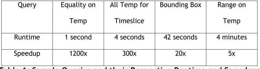
answer in only 4 minutes, still five times faster than previously possible. See table 1
for some example queries and the time needed to complete them, as well as the
amount of speedup demonstrated versus a complete file scan.
Query Equality on
Temp
All Temp for
Timeslice
Bounding Box Range on
Temp
Runtime 1 second 4 seconds 42 seconds 4 minutes
Speedup 1200x 300x 20x 5x
Table 1: Sample Queries and their Respective Runtime and Speedups
As can be seen above, for a nominal amount of creation time, a bitmap index of a
netCDF file can be created allowing for an otherwise unobtainable level of interactive
access to the data contained within. This access further makes it possible to perform
even more complex operations upon the dataset, such as the similarity searches
Chapter 4: Implementation and Viewing of Spatio-Temporal Queries
Recent studies[6] on the query processing of mesh data (such as data stored in
netCDF files) identify four classes of primitive operations, temporal, spatial,
proximity, and statistical. Implementations for each of these classes within the
integrated netCDF-FastBit framework established in chapter 3 are discussed below.
Further, the process of visualizing the resulting output from the submitted queries is
discussed, along with some example visualizations.
4.1 Temporal Operations
As their name suggests, Temporal Operations are operations intended to
function along the dimension of time. Three simple examples of this would be the
concepts of before, after, and during.
NetCDF does not utilize any built in date data type; however, as the data involved is
very often of a geospatial-temporal nature some measure of time is needed.
Generally this is achieved utilizing the standard measure of UNIX time[17] (the number
of seconds since January 1st, 1970) or some variant thereof. This means temporal
operations can be generalized down to simple arithmetic problems between two
integers. In order to search for events or measurements before a certain time, one
would only have to convert the desired date into its corresponding integer and submit
a search specifying interest only in time values less than the provided value. Likewise,
it is simple to search a span of time by indicating an interest only in results that fall
simple equality comparisons FastBit can efficiently select out only those data points
falling within the time of interest.
As an example, to only return results from a specific time slice, the clause
time = X could be appended in the Where statement, ensuring that any values
returned would have been observed at the given point in time. To construct a query
specifying a time before or after the given time the equals sign would simply need to
be replaced using a less than or greater than signs. A span of time could be indicated
using X < time < Y, which would indicate returned values should have been measured
between the two points in time specified.
4.2 Spatial Operations
Spatial Operations offer up a close analogue to the Temporal Operations
mentioned in the last section, except they apply to the three special dimensions. A
common concept within spatial operations is a bounding box, a set of four coordinates
which form a box that is then useful within the context of spatial operations. Several
relations can be defined using a bounding box, such as contained by, disjoint, or
overlapping.
As our netCDF files of interest contain data relating to meteorological conditions upon
the globe of the Earth, latitude and longitude measurements provide convenient
methods for defining a spatial location on the globe from which a data measurement
or reading was observed. Similarly, for data taken not only along different longitude,
performed under the sea, or perhaps even under ground) simple integer variables can
easily store a numerical depiction of the location. Just as with the temporal
operations, it is easy for FastBit to construct simple equality comparisons between
any of these dimensions, in any possible configuration. While FastBit does not
implement any standard spatial search features, such as a bounding box search, they
are very easily to replicate using two-sided inequalities.
A bounding box search for all points with a box that stretched from longitude,
latitude points (0, 0) to (20, 20) could be expressed within FastBit as
0 <= latitude <= 20 and 0 <= longitude <= 20.
A three dimensional element could be easily introduced, either to create a "bounding
cube" instead, or to specify a single level of elevation within which to perform the
bounding box search. For other spatial shapes a list of OR'd longitude, latitude points
would be used to describe the path and shape traversed by the shape. By simply
reversing the above query for points within the bounding box from (0, 0) to (20, 20)
we can create
(0 >= latitude or latitude >= 20) and (0 >= longitude or longitude >= 20)
4.3 Proximity Operations
While the last two classes of operations dealt mainly with locating points whose
coordinates shared a specified relationship with another given set of coordinates,
Proximity Operations represent a more complicated problem. Instead of looking for
direct relationships between two sets of coordinates Proximity Operations perform
comparisons between a data points coordinates, returning values close to the
specified point utilizing a given metric, in this case physical distance.
As seen from the previous two sections, FastBit's subset of SQL easily and efficiently
handles queries involving equalities. What is more problematic is when instead of
having a specific set of longitude, latitude points, the user possesses a single
longitude, latitude point and a measurement of distance around which they are
interested. Determining which points fall within this specified range is complicated,
not only because longitude and latitude do not directly correspond to any commonly
used measurement of distance, but also because, due to the curved nature of Earth's
surface, calculating the range between them is not a matter of simple addition or
subtraction (as it would be if longitude, latitude points represented points on a grid
rather than points upon a sphere). Similar problems appear frequently in many fields,
particularly those related to navigation, where knowledge of what objects lie within a
specified distance provides an obvious utility.
haversine(d/R) = haversine(∆latitude) +
cos(latitude1)cos(latitude2)haversine(∆longitude),
which computes the great-sphere distance (the shortest distance over the surface of a
sphere) of two points located on the globe, utilizing the points’ longitude, latitude
values. In this formula the variable d represents the distance between the two points
while R is the radius of the sphere itself. Since in this case we are interested in d, the
distance between two longitude, latitude points, we can solve the haversine formula
for d, which results in
d = 2Rhaversin-1(h) = 2Rsin-1(√h).
This can be expanded further to
d = 2Rsin-1(√(sin2(∆latitude/2) + cos(latitude1)cos(latitude2)sin2(∆longitude/2).
Using 3,956 miles as an estimate of Earth's radius we can express the previous
expanded formula using built in mathematical functions found within FastBit's SQL
implementation, giving us this SQL statement,
2 * 3956 * asin(sqrt(pow(sin((specified latitude - latitude) * 0.0174/2), 2) +
cos(specified latitude * 0.0174/2) * cos(latitude * 0.0174/2) * pow(sin((specified
The specified latitude and longitude mentioned in the formula refer to the longitude,
latitude point from which the range is being measured. It is a simple matter to create
a shell script that can accept two variables and submit the above SQL statement to
FastBit, inserting the provided latitude and longitude where appropriate within the
query. The presence of 0.0174 repeatedly throughout the SQL statement is merely to
convert the decimal representations of latitude and longitude found within the data
itself into radians, by multiplying by an approximation of pi divided by 180. In cases
where the longitude and latitude were stored within the netCDF file already in
radians, the values should be left off. By using this SQL query within the Select
statement, this formula will compare the specified longitude, latitude point against
every longitude, latitude point within the dataset and calculate the distance between
them, presenting the results in a new column, named distance in this instance.
Returning to the original problem at hand, those points within our range of interest
can then be easily picked out by an additional clause in the Where statement,
distance <= X, thus returning the values for those longitude, latitude points that lie
no more than the specified distance away from our starting point. Obviously,
however, this formula represents a heavy computational load, which must be applied
between the given longitude, latitude point and every longitude, latitude point within
the dataset.
With even a reasonably sized dataset, this computational cost can rapidly become
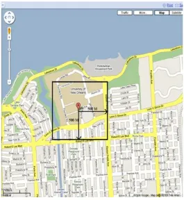
step filtration process is proposed. First, a rough estimate will be applied that will
include every longitude, latitude point within the area of interest as well as several
outside. It is estimated[4] that each degree of latitude is roughly equivalent to 69
miles, while each degree of longitude is equivalent to the cosine of the latitude
multiplied by 69 miles. Using these estimates we can construct a bounding box that
will always possess all longitude, latitude points within the specified distance of the
starting point, as depicted in Figure 6, and express it in FastBit acceptable SQL as
(specified latitude - range/69) <=latitude <= (specified latitude + range/69) and
(specified longitude - range/cos(specified latitude) * 69) <= longitude <= (specified
longitude + range/cos(specified latitude) * 69).
By adding these two clauses into the Where statement of the SQL query, a bounding
box is formed that subsets the points within the dataset. This subset of the entire
dataset's longitude, latitude points will then be given to the second filter, the
haversine function presented above, so that those points further from the specified
point than the given distance can be removed from the final results. By applying this
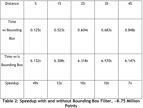
two step filter to the Range query devised here, very large speedups are
demonstrated within the runtimes of the queries, alleviating the time requirements of
using the haversine Range query by itself. This speedup is, as expected, greater the
more points it can manage to exclude from the haversine function used to compute
space defined within the file, speedup will be very limited. Table 2 and 3 depict the
time needed and speedup obtained using this bounding box filter.
Distance 5 15 25 35 45
Time
w/Bounding
Box
0.125s 0.523s 0.604s 0.683s 0.848s
Time w/o
Bounding Box
6.132s 6.308s 6.318s 6.570s 6.147s
Speedup 49x 12x 10x 10x 7x
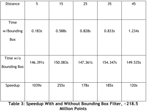
Distance 5 15 25 35 45
Time
w/Bounding
Box
0.183s 0.588s 0.828s 0.833s 1.234s
Time w/o
Bounding Box
146.391s 150.083s 147.361s 154.347s 149.535s
Speedup 1039x 255x 178x 185x 120x
Table 3: Speedup With and Without Bounding Box Filter, ~218.5
Million Points
Having devised a method by which all points within a certain distance of a given point
can be returned, we can now extend this Range query further to produce a
pseudo-KNN. By sorting the returned results according to ascending distance, and limiting
them to the first K results, our returned longitude, latitude points contain only the K
nearest points to the starting point. While superficially resembling a KNN search, this
search will return the K nearest neighbors, no matter the distance separating them.
This search, however, will only return the K nearest neighbors within a given range. It
is certainly possible that less than K points will be within the range specified if the
range is particularly small, or the dataset does not cover the area of interest evenly.
To enhance the usability of these large complicated SQL statements, an easy to use
shell script was created so that a user merely needs to identify the longitude, latitude
point of interest, as well as a range around the point to search. While created solely
for testing purposes, the script can be extended to easily substitute the haversine
formula and bounding box filter into any query requiring either a Range or
pseudo-KNN search.
4.4 Statistical Operations
When dealing with large amounts of data, it is often useful to be able to
provide some level of statistical analysis relating to the data as a whole. This kind of
analysis allows for the understanding of trends within the data, and provides for the
ability to not only forecast future changes within the data, but to also explain on a
deeper level precisely how the disparate data points interact with one another. By
collecting and analyzing various data points, Statistical Operations can offer new ways
of presenting and viewing pieces of data, allowing for more accurate interpretations
of how and why the data points are changing.
By default, FastBit implements four Statistical Operations within its default SQL
over a period of time, Avg(temperature) would provide the average temperature
over the entire time span. Max instead gives the maximum value held over the entire
column, and extending the previous example, could be utilized to find the highest
temperature over the measured time span. Min acts as Max's opposite, and instead
finds the minimum value over an entire column. Again, looking back to the previous
example, Min could be used to find the lowest temperature during the period of
observation. Finally, Sum presents all of the values within the column, summed
together. In the context of the example used so far this function has little relevance
as providing the summed total of all temperatures over a time period does not relay
any useful information. For other calculations, however, Sum can be a useful tool, for
example, providing the total amount of rainfall in an area over a period of time.
When utilizing any of these Statistical Operations, FastBit performs an implicit SQL
Group By clause, utilizing any of the selected variables not appearing within a
statistical function. Finally, a column is appended to the results generated utilizing
these Statistical Operations with a Count of the number of rows utilized in
determining their values.
In addition to this array of Statistical Operations, other complex statistical
calculations can be built utilizing these default four operations as basic building
blocks. The most frequently appearing value for a data column, the Mode, can be
calculated by selecting the column in question as well as its Avg.
The resulting SQL statement will be similar to select temp, avg(temp) sort by desc
the resulting column in descending order, the most frequently occurring value may be
found. Other Statistical Operations will require changes to FastBit’s current parser for
SQL queries, or an alternate function which can accept the results of several queries
and produce the desired value. Computing the Standard Deviation, for example,
would currently be impossible as FastBit could not determine what the differences
between a column of values and the average of those values is.
4.5 Visualization
The resulting output from any of the operations discussed above, or for any
operation upon FastBit in general, is a set of comma separated values output to either
screen or file. For the most part, however, this kind of output is difficult to use, or
even understand, without some kind of additional help. To advance towards that goal
the process of visualization was suggested.
With the aid of Fareed Qaddoura 2D and 3D visual representations from the test 1.4
GB netCDF file were created using raster layers created for each specified variable in
the netCDF file. For animating purposes, a time series raster was created from
another specified variable, then applied using ESRI’s arcscene[19] animation manager.
Figure 7 presents an example of a 2D visualization, while Figure 8 depicts a 3D
Chapter 5: Conclusions and Future Work
5.1 Future Work
There remains many different ways in which this project could be expanded
even further. Currently the processes discussed throughout this paper have been
written externally to the GUI as presented in Chapter 2. A large amount of work could
be expended bringing these external processes within the proposed GUI and made
native to that interface. Further, the visualization discussed in Chapter 4 must still be
created largely by hand, as ESRI’s ArcGIS desktop suite cannot directly read netCDF or
comma separated files. As such, a user is currently required to interpret both the
metadata within the netCDF file as well as the comma separated value results from
FastBit for the creation of the visualization step’s raster layers. For the purposes of
further visualization, a way to incorporate the input comma separated value FastBit
output into the visualization process is needed. It is likely scripts could be
implemented to create the visuals. Based on the outcome of the previous steps, the
proposed GUI’s design will need to be updated.
For purposes of netCDF and FastBit integration, a tighter coupling between them
should also be possible. The trimmed ncks tool may have room for further cuts, finally
allowing it to be wholly contained within FastBit and eliminating the need for shell
scripts, sockets, or any other extraneous tools outside of FastBit itself. Alternatively,
the ncks tool (the original or trimmed version) could serve as a template for the
purpose of utilizing it with FastBit that it can be kept to a suitable size, or that the
layout of FastBit can be arranged so as to not unduly burden the rest of the tool set.
While both the solution utilized within this project and the two suggestions found just
above still employ converting netCDF data to comma separated value formatted lines
and feeding that to FastBit, a third possible alternative would be to alter FastBit itself
so it could read netCDF directly. There is no technical reason FastBit can only
interpret comma separated values, and it should be eminently possible to create
native netCDF support within FastBit. This third option will require a very in depth
understanding of how both netCDF and FastBit work, however, far more than is
required for options utilizing already prevalent options.
Another source of continued work is the extension of the columns loaded in this
manner. Currently, the ncks tool only allows for the conversion of one variable from
netCDF to comma separated value format at a time. While this means that one could
use ncks to create comma separated values for all of the values and coordinate
dimensions of a single variable, for example converting time, depth, latitude, and
longitude as well as the temperature values for the water_temp variable, one could
not also convert the salinity variable simultaneously. This inherently limits the type of
queries possible within our current setup, as only one variable is able to be
referenced using any given query. It is possible to use ncks to export only one
variable, formatted in such a way as to enable its addition to an already existing
FastBit bitmap index but unfortunately there is currently no programmatic interface
alteration to FastBit to enable programmatic support would be of great use in this
area, or alternatively the formulation of a shell script that could perform the needed
actions. Yet another alternative approach to this problem would be to try and alter
the ncks tool to support the conversion of more than one variable at the same time;
this, however, would require very extensive knowledge not only of netCDF but of the
nco tools themselves.
In the operations category, there also remains ample room for expansion through
future work. Many statistical operations exist which are still beyond the capabilities
of FastBit, such as computations to find the Standard Deviation or Variance of a
dataset. While this information can be found using with standard SQL operations,
FastBit's limited implementation of SQL lacks the capacity to generate these values.
Currently, to find the Standard Deviation of a dataset, for example, one would need
to collect the output from one or more queries and then do the final computations
manually. Obviously, this is an area that could be further built upon, either by
implementing these capabilities into FastBit itself, or creating a process to
automatically collect and compute the Standard Deviation from prepared FastBit
output. Likewise, while the context of the work within this project, meteorological
netCDF datasets, did not make use of heavily detailed geometric shapes, the
implementation of these features is eminently possible within FastBit. Currently every
point within the shape would need to be selected for explicitly, forming a long
generate these statements could prove useful for the utilization of these operations
on more detailed geospatial bit mapped data.
Returning to the system architecture as proposed above in Chapter 2, much of the
suggested layout has been built in the work above. One area that presents a viable
source of future work, however, is the Metadata Repository. NetCDF files, by
convention, hold varying amounts of metadata within their header. It should be
possible to support one or more conventions for metadata layout within netCDF
headers for use with the proposed Metadata Repository. Another area of possible
expansion lies in the forms of output provided by the Query Processor. The interface
of the project itself could also use refinement, transitioning away from the command
line interface currently in use and towards the GUI initially proposed instead.
5.2 Conclusions
As has been demonstrated, the use of FastBit bitmap indexing with netCDF
meteorological data offers fast and efficient search capability otherwise unavailable
to users. The user can customize the generated index to emphasize certain types of
queries or to better handle different sets of data. The SQL interface implemented
within FastBit allows for a large amount of flexibility in the queries that can be
created, and has been shown to support four classes of primitive operations. The two
step filtering algorithm provides for a large speedup when utilized with the haversine