Demographic Researcha free, expedited, online journal of peer-reviewed research and commentary
in the population sciences published by the Max Planck Institute for Demographic Research Konrad-Zuse Str. 1, D-18057 Rostock·GERMANY www.demographic-research.org
DEMOGRAPHIC RESEARCH
VOLUME 23, ARTICLE 3, PAGES 63-72
PUBLISHED 09 JULY 2010
http://www.demographic-research.org/Volumes/Vol23/3/ DOI: 10.4054/DemRes.2010.23.3
Formal Relationships 9
Sensitivity of life disparity with respect to
changes in mortality rates
Peter Wagner
This article is part of the Special Collection “Formal Relationships”. Guest Editors are Joshua R. Goldstein and James W. Vaupel.
c
°2010 Peter Wagner.
2 Relationship 65
3 Proof 66
4 History and related results 69
5 Applications 70
Formal Relationships 9
Sensitivity of life disparity with respect to changes in mortality rates
Peter Wagner1,2
Abstract
This article is concerned with sensitivity analysis of life disparity with respect to changes in mortality rates. A relationship is derived that describes the effect on life disparity caused by a perturbation of the force of mortality. Recently Zhang and Vaupel introduced a “threshold age”, before which averting deaths reduces disparity, while averting deaths after that age increases disparity. I provide a refinement to this result by characterizing the ages at which averting deaths has an extremal impact on life disparity. The results are illustrated using data for the female populations of Denmark in 1835, and for the United States in 2005.
1Max Planck Institute for Demographic Research, Konrad-Zuse-Straße 1, 18057 Rostock, Germany. E-mail:
2The author thanks Carl Schmertmann for thoughtful recommendations, including the interpretation of the
1. Introduction
In keeping with Keyfitz’s idea that everybody dies prematurely, since every death deprives the person involved of the remainder of his expectation of life (Keyfitz 1977:61-68), the measuree†for the average life expectancy lost due to death has been widely studied. It first appeared in Mitra (1978) and was developed further by Vaupel (1986) and recently in Vaupel and Canudas-Romo (2003), Zhang and Vaupel (2008) and Shkolnikov et al. (2009). Zhang and Vaupel (2009) initiated a new direction of analysis, studying the impact one†of a concentrated decrease in mortality at agea.
Life disparity is measured by life expectancy lost due to death
(1) e†=
Z ∞
0
e(x)d(x)dx,
wheree(x)is the remaining life expectancy at agex,
(2) e(x) = 1
`(x) Z ∞
x
¡
y−x¢d(y)dy= 1
`(x) Z ∞
x
`(y)dy,
`(x) = exp (−H(x))is the probability of survival to agex,H(x) =R0xµ(y)dyis the cumulative hazard function andµ(x)is the age-specific hazard of death. Since nobody lives forever, it is generally assumed thatHis strictly increasing, attaining all non-negative real numbers. The functiond(x) = d
dx
¡
1−`(x)¢=`(x)µ(x)is the life table distribution of deaths.
Goldman and Lord (1986: equations (6), (14)) and Vaupel (1986: equations (4), (5)) independently showed that life disparity (1) is the product of the life expectancy at birth and the entropy of the life table
(3) e†=e(0)
Ã
−
R∞
0 `R(x) log`(x)dx
∞
0 `(x)dx
!
.
2. Relationship
Letϕ(a)represent the change ofe† caused by a reduction in mortality at agea(with a precise definition thereof via a limit of derivatives given in the proof). The main relationship in this article consists of two equivalent formulae ((4), (5)) for the functionϕ.
Theorem 1
The functionϕ(a), representing the change ofe† caused by a reduction in mortality at agea, satisfies the relationship
(4) ϕ(a) =−
Z ∞
a `(x)
³
1 + log`(x) ´
dx
and, equivalently,
(5) ϕ(a) =`(a) ³
H(a)e(a)−e(a) +e†(a) ´
,
wheree†(a)denotes life expectancy lost due to death among people surviving to agea,
(6) e†(a) = 1
`(a) Z ∞
a
e(x)d(x)dx.
Furthermore,ϕhas the following three properties:
(i) Monotonicity
Let˜a, the age of cumulative hazard unity, be defined viaH(˜a) = 1. Thenϕis strictly increasing on[0,˜a]and strictly decreasing and strictly positive on[˜a,∞), having a global maximum ofϕ(˜a) = exp(−1)e†(˜a)ata= ˜aand a local minimum ofϕ(0) =e†(0)−e(0) ata= 0. More precisely,
(7) d
daϕ(a) =`(a)
¡
1−H(a)¢.
(ii) Curvature
Leta∗be defined byH(a∗) = 2. Thenϕis strictly concave on[0, a∗]and strictly convex on[a∗,∞). More precisely,
d2
da2ϕ(a) =d(a)
¡
H(a)−2¢.
(iii) Asymptotic Behaviour
lim
Zhang and Vaupel (2009) showed that, if the life table entropy (cf. (3)) satisfies
e†/e(0)<1, then there exists a positive “threshold age”a†between the regions of “early” agesa < a†, in which the effect of averting deaths on life disparity is negative, and “late” agesa > a†, in which this effect is positive. Ife†/e(0) = 1, thena† = 0, and the effect is positive at all ages other than zero. Finally, ife†/e(0)>1, thena†does not exist, and the effect is positive everywhere. Refining these results, Theorem 1(i) highlights some helpful monotonicity properties and draws attention to˜aand0, the ages of extremal effect on life disparity caused by averting deaths.
Remark 1
Recall definition (1) and think ofe†as the sum of three integrals, by partitioning the range of integration into the ages below, at and abovea. It turns out that the three summands in equation (5) correspond to the effects of a mortality reduction at ageaon the three integrals, which I shall refer to as the “early”, “instant” and “late” effect, respectively:
• Early: At agesx < a, deathsd(x)are unchanged, and life expectancies of survivors
e(x)increase, whichincreasesdisparity by`(a)H(a)e(a).
• Instant: At agex=a, deathsd(x)decrease, and life expectancy of survivorse(x)is unchanged, whichdecreasesdisparity by`(a)e(a).
• Late: At agesx > a, deathsd(x)increase, and life expectancies of survivorse(x)are unchanged, whichincreasesdisparity by`(a)e†(a).
3. Proof
Theorem 1, the relationship
In the general case, the force of mortalityµchanges by some function∆µ, with a small steps:
µ(x, s) =µ(x) +s∆µ(x),
µs(x, s) = ∂
∂sµ(x, s) = ∆µ(x).
(8)
Similarly, for thes-dependent survival function,
`(x, s) = exp µ
−
Z x
0
µ(y, s)dy
¶
,
`s(x, s) = µ
−
Z x
0
∆µ(y)dy
¶
Notinge† =e†(0)(cf. (1), (6)), by equation (3),
e†(0, s) =−
Z ∞
0
`(x, s) log`(x, s)dx.
Hence
e†
s(0, s) =−
Z ∞
0
`s(x, s)¡1 + log`(x, s)¢dx
=− Z ∞ 0 µ − Z x 0
∆µ(y)dy
¶
`(x, s)¡1 + log`(x, s)¢dx
= Z ∞
0
∆µ(y) µZ ∞
y
`(x, s)¡1 + log`(x, s)¢dx
¶
dy.
Thus the functional derivative of disparity with respect to mortality change∆µis
e†
s(0,0) =
Z ∞
0
∆µ(y) µZ ∞
y
`(x)¡1 + log`(x)¢dx
¶
dy.
Keeping mortalityreductions at ageain mind, when∆µis a negative step function in a small neighbourhood around agea, such that its integral equals minus unity; for example, and from now on,∆µ(y) =−1/εfory∈[a, a+ε]and zero elsewhere, then
e†s(0,0) =
1 ε Z a+ε a µ − Z ∞ y
`(x)¡1 + log`(x)¢dx
¶
dy ∼ −
Z ∞
a
`(x)¡1+log`(x)¢dx
or, more precisely, and hereby definingϕ(a)as a limit of derivatives,
ϕ(a) = lim
ε→0e
†
s(0,0) =−
Z ∞
a
`(x)¡1 + log`(x)¢dx.
Finally, note that
−
Z ∞
a
`(x)(1 + log`(x))dx=`(a) µ
−
Z ∞
a `(x)
`(a) ³
log`(a) + 1 + log`(x)
`(a) ´
dx
¶
Theorem 1, part (i)
By equation (5),ϕis strictly positive on[˜a,∞). Equation (7) follows from equation (4), so that the first derivative ofϕis strictly positive on[0,a˜)and strictly negative on(˜a,∞). Thus,ϕis strictly increasing on[0,˜a]and strictly decreasing on[˜a,∞). Consequently,ϕ
has a global maximum ata= ˜aand a local minimum ata= 0with
ϕ(˜a) =`(˜a)e†(˜a) = exp(−1)e†(˜a) and ϕ(0) =e†(0)−e(0).
Theorem 1, part (ii)
Differentiating equation (7) with respect toa,
d2
da2ϕ(a) =−d(a)
¡
1−H(a)¢−`(a)µ(a) =d(a)¡H(a)−2¢.
Hence the second derivative ofϕis strictly negative on[0, a∗)and strictly positive on
(a∗,∞). Thus,ϕis strictly concave on[0, a∗]and strictly convex on[a∗,∞).
Theorem 1, part (iii)
Clearly, both the “instant” and “late” effect (cf. (2), (6)) approach zero, that is,
lim
a→∞
³
−`(a)e(a) ´
= 0 and lim
a→∞
³
l(a)e†(a)´= 0,
so that, by equation (5), it remains to show
lim
a→∞
³
`(a)H(a)e(a) ´
= 0
for the “early” effect`(a)H(a)e(a). Using integration by parts,
e† =
Z ∞
0
e(x)d(x)dx= Z ∞
0 µ(x)
³
`(x)e(x) ´ dx = ³ lim x→∞ ³
H(x)`(x)e(x) ´ −0 ´ + Z ∞ 0
H(x)`(x)dx,
where, by reversing the order of integration,
Z ∞
0
H(x)`(x)dx= Z ∞
0
µZ x
0
µ(y)dy
¶
`(x)dx= Z ∞
0
µZ ∞
y
`(x)dx
¶
µ(y)dy
= Z ∞
0
`(y)e(y)µ(y)dy= Z ∞
0
4. History and related results
For a concise introduction to functional derivatives see, for example, Arthur (1984) and Frigyik, Srivastava, and Gupta (2008), with applications of the mathematical techniques used here to demography and subjects such as engineering, respectively.
Recall that the perturbation (8) for my specific choice of∆µrepresents anabsolute reduction of the death rate on the age interval[a, a+ε]. A reduction of the death rate on the same intervalrelativeto its value at ageais given by
˜
µ(x, s) =µ(x) +s µ(a) ∆µ(x) =µ(x, s µ(a)).
Then
g(a) = lim
ε→0˜e
†
s(0,0) = limε→0
µ
∂ ∂se˜
†(0, s)
¯ ¯ ¯ ¯ s=0 ¶ = lim
ε→0
µ
∂ ∂se
†(0, sµ(a))
¯ ¯ ¯ ¯ s=0 ¶ = lim
ε→0
µ
µ(a) ∂
∂se
†(0, s)
¯ ¯ ¯ ¯ s=0 ¶
=µ(a) lim
ε→0e
†
s(0,0) =µ(a)ϕ(a)
=d(a)³H(a)e(a)−e(a) +e†(a)´,
which is equation (2) in Zhang and Vaupel (2008). Letting
k(a) =H(a)e(a)−e(a) +e†(a)
(Zhang and Vaupel 2008: equation (3)), motivated by data for Japanese females in 1950, 1970 and 1990, Zhang and Vaupel discuss implications of the existence of a unique root ofk, a so-called “threshold age”, forg, the “age-specific impact of survival improvement on lifespan disparity”.
In Zhang and Vaupel (2009), a formal proof for the existence of at most one root ofk
is given. Their derivation of the relationship fork(Zhang and Vaupel 2009: equation (1)) is based on an absolute “concentrated decrease in mortality at agea”, in my notation corresponding to
∂ ∂s
³ lim
ε→0e
†(0, s)´¯¯¯
¯
s=0 ,
which turns out to equal
lim
ε→0
µ
∂ ∂se
†(0, s)
¯ ¯ ¯ ¯ s=0 ¶
Although in this case, the order of the two limiting processes does not matter, their demographic interpretations differ. First differentiating and then lettingεtend to zero describes the impact of an absolute mortality decrease over a narrower and narrower age range starting at agea. However, first lettingεtend to zero and then differentiating raises the challenge of having to interpret cumulative hazard functions with a downward step,
Ha,s(x) =H(x)−s·1[a,∞)(x)
(where1[a,∞)(x)is one forx≥aand zero otherwise), and negative death rates, possibly
by (rather hypothetically) resurrecting some of a cohort’s decedents. The latter approach of Zhang and Vaupel (2009) was also taken in Wagner (2010), where the new value of life disparity (corresponding to theHa,s(x)above) was shown to satisfy
e†a,s=e†+
¡
exp(s)−1¢`(a) ³
H(a)e(a)−e(a) +e†(a) ´
,
from which it follows immediately that
∂ ∂se
†
a,s
¯ ¯ ¯ ¯
s=0
=`(a)³H(a)e(a)−e(a) +e†(a)´=ϕ(a).
Regardless of the origin of the simple relationϕ=`·k, implying thatϕandkalways have the same sign, it is striking how much more information can be obtained forϕ, in terms of monotonicity, curvature, and asymptotic behaviour, as summarised in Theorem 1.
5. Applications
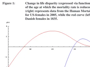
To illustrate the theoretical results, I have computed several relevant quantities for life tables from the Human Mortality Database (2010). Since the functionϕis very similar for populations of one and the same era, essentially sharing the same kind of mortality schedule, I concentrate on displayingϕfor a contemporary against a historical table. In my Figure 1, the blue curve representsϕfor the female population of the United States in 2005, wherea† ∼78.59and˜a∼ 87.42, whereas the red curve representsϕfor the population of Danish females in 1835, wherea† ∼34.02and˜a∼60.36. Note that my Figure 1 concurs with Figures 1 and 2 of Zhang and Vaupel (2009).
Figure 1: Change in life disparity (expressed via function (5)) as a function of the age at which the mortality rate is reduced. The blue curve (right) represents data from the Human Mortality Database 2010 for US-females in 2005, while the red curve (left) corresponds to Danish females in 1835.
References
Arthur, W.B. (1984). The analysis of linkages in demographic theory.Demography21(1): 109–128.doi:10.2307/2061031.
Frigyik, B.A., Srivastava, S., and Gupta, M.R. (2008). An introduction to functional derivatives. University of Washington, Department of Electrical Engineering. (UWEE Technical Report Number UWEETR-2008-0001).
Goldman, N. and Lord, G. (1986). A new look at entropy and the life table.Demography 23(2): 275–282.doi:10.2307/2061621.
Human Mortality Database (2010). [electronic resource]. University of California, Berkeley, USA and Max Planck Institute for Demographic Research, Rostock, Germany. Available at www.mortality.org or www.humanmortality.de. Downloaded on January 7, 2010.
Keyfitz, N. (1977).Applied Mathematical Demography. New York: John Wiley. Mitra, S. (1978). A short note on the Taeuber paradox. Demography15(4): 621–623.
doi:10.2307/2061211.
Shkolnikov, V.M., Andreev, E.M., Zhang, Z., Oeppen, J., and Vaupel, J.W. (2009). Losses of expected lifetime in the US and other delevoped countries: methods and empirical analyses. Rostock: Max Planck Institute for Demographic Research. (MPIDR working paper WP 2009-042).
Vaupel, J.W. (1986). How change in age-specific mortality affects life expectancy.
Population Studies40(1): 147–157. doi:10.1080/0032472031000141896.
Vaupel, J.W. and Canudas-Romo, V. (2003). Decomposing changes in life expectancy: A bouquet of formulas in honor of Nathan Keyfitz’s 90th birthday. Demography40(2): 201–216.doi:10.1353/dem.2003.0018.
Wagner, P. (2010). The ages of extremal impact on life disparity caused by averting deaths. Rostock: Max Planck Institute for Demographic Research. (MPIDR working Paper WP 2010-016).
Zhang, Z. and Vaupel, J.W. (2008). The threshold between compression and expansion
of mortality. Paper presented at the Population Association of America 2008 Annual
Meeting, New Orleans, April 17-19, 2008.
Zhang, Z. and Vaupel, J.W. (2009). The age separating early deaths from late deaths.