AUT J. Model. Simul., 49(2)(2017)1-2 DOI: 10.22060/mej.2016.503
Partial Observation in Distributed Supervisory Control of Discrete-Event Systems
V. Saeidi, A. Afzalian, D. Gharavian
Dept. of Electrical Engineering, Abbaspour School of Engineering, Shahid Beheshti University, Tehran, Iran
ABSTRACT: Distributed supervisory control is a method to synthesize local controllers in discrete-event systems with a systematic observation of the plant. Some works were reported on extending this method by which local controllers are constructed so that observation properties are preserved from monolithic to distributed supervisory control, in an up-down approach. In this paper, we find circumstances in which observation properties are preserved from monolithic to distributed supervisory control. Local observation properties, i.e. local normality and local relative observability are employed for investigating observation properties of each local controller, which are constructed by any localization algorithm that preserves control equivalency to the monolithic supervisor with respect to the plant. These properties enable us to investigate the observation properties from monolithic to distributed supervisory control. Moreover, observation equivalence property is defined according to the control equivalence in a distributed supervisory control with partial observation. It is proved that with preserving observation equivalence of the local controllers to the monolithic supervisor, the control equivalence is satisfied, if and only if the intersection of local event sets is a subset of or equal to the global observable event set.
Review History: Received: 16 October 2016 Revised: 24 February 2017 Accepted: 27 February 2017 Available Online: 12 March 2017
Keywords:
Distributed Supervisory Control Local Normality
Local Relative Observability Observation Equivalent
1- Introduction
The supervisory control theory handles small scale discrete event systems (DES) [1], Since, in the large scale DES the number of states grows with the number of components. Supervisory control synthesis for the monolithic specification encounters with computational complexity. In order to overcome the computational complexity, modular and decentralized [2, 3], hierarchical [4,5] and heterarchical [6-9] approaches have been proposed in the supervisory control of DES. The decentralized supervisory control scheme reduces the computational complexity in large scale DES [10, 11]. Since a decentralized supervisor observes the plant partially, he does not have enough information about the other supervisors, and their decisions may be in conflict with each other. In [9], a method was introduced for synthesizing the optimal non-blocking decentralized supervisory control using Lm-observer and output control consistency (OCC) properties. In [11], decomposability and strong decomposability (conormality) were defined to construct the decentralized supervisory control in a top-down approach. Other accessible properties are co-observability and relative co-observability which were defined in [11] and [12], respectively. In order to remove conflict between decentralized supervisors, construction of a coordinator was proposed in the literature [13, 14]. In [15], a supervisor localization procedure was proposed to guarantee the optimality and the non-conflicting of the local controllers and the monolithic supervisor.
Observation properties e.g. normality [16], observability [16] and relative observability [17] describe the effect of observation on the control behavior.
The authors of [15] developed a Distributed supervisory control based on localization of the monolithic supervisor with full observation. The paper [18] proposed a method for recognizing the conflicts between the supervisors, using the observer property of a natural projection
In [19], an abstraction method was proposed to construct a distributed supervisory control (in a top-down approach), in which the observation properties of monolithic supervisor is preserved in local controllers. In the present study, We find circumstances for preserving observation properties in local controllers, constructed by supervisor localization procedure [15], or constructed by decomposition of the monolithic supervisor [11].
applications, such as gas transmission networks and power systems [22].
In the rest of the paper, necessary preliminaries are reviewed in section 2. In order to redefine the observation properties by set algebra approach, some formulations are introduced in section 3. Observation properties in distributed supervisory control are redefined by a set algebra approach in section 4. The observation equivalence is introduced and is compared with control equivalence in section 5. In section 6, the extended theorem is illustrated by some examples. Finally, the concluding remarks are presented in section 7.
2- Preliminaries
The set of all finite strings over Σ is denoted Σ*. The concatenation of two strings s1,s2⊆Σ* is written as s1 s2⊆Σ* and s1≤s, where s1 is the prefix of s. ϵ∈Σ* is the empty string,
and sϵ=ϵs=s does hold. A DES is introduced by an automaton G=(Q,Σ,δ,q0,Qm) in which Q is a finite set of states, with q0∈Q
as the initial state and Qm⊆Q being the desired (marked)
states. Σ is a finite set of events, and finally δ is a transition mapping δ:Q×Σ→Q∶ δ(q,σ)=q`. L(G)≔{s∈Σ*│δ(q
0,s)!} is the closed behavior of G and Lm (G)≔{s∈L(G)│δ(q0,s)∈Qm} is the marked behavior of G.
The natural projection is a mapping P:Σ*→Σ
0* where
(1) P(ϵ):=ϵ ,(2) for s∈Σ*,σ∈Σ ,P(sσ):=P(s)P(σ), and (3)
P(σ):=σ if σ∈Σ0 and P(σ):=ϵ if σ∉Σ0. The effect of P on the string s∈Σ* is to erase the events in s that do not belong
to the observable event set Σ0. The natural projection P
can be extended and denoted by P:Pwr(Σ*)→Pwr(Σ 0*). For any X⊆Σ*, P(X)≔{P(s)│s∈X}. The inverse image function of P is denoted by P-1:Pwr(Σ
0*)→Pwr(Σ*) and P-1(X)≔{s∈Σ*│P(s)∈X}. The synchronous product of languages L1⊆Σ1* and L2⊆Σ2* is defined by L1∥L2=P1 -1(L
1)∩P2-1(L2)⊆Σ*, where Pi:Σ*→Σi*,i=1,2 for the union
Σ=Σ1∪Σ2 [9,23].
In the supervisory control context, all events in Σ are partitioned as a set of controllable events Σc and a set of
uncontrollable events Σuc, where Σ=Σc⨃Σuc. A control pattern
is γ, where Σuc⊆γ⊆Σ and the set of all control patterns is
denoted by Γ={γ∈2Σ│γ⊇Σ
uc}. A supervisor for G is a map
V:L(G)→Γ, where V(s) represents the set of enabled events after the occurrence of the string s∈L(G). Namely, a supervisor only disables the controllable events. A pair (G,V) is written as V/G and called “G that is under supervision of V”. The closed loop language L(V/G) is defined by: (1) ϵ∈L(V/G) (2) sσ∈L(V/G) iff s∈L(V/G), σ∈V(s), and sσ∈L(G). The marked strings of V/G is defined as Lm(V/G)=L(V/G)∩Lm(G). The closed loop system is non-blocking if is the set of all prefixes of traces in Lm(V/G). A language K⊆Σ* is controllable with respect to (w.r.t.)
L(G) and Σuc, if K̅Σuc∩L(G)⊆K̅. The set of all controllable
sublanguages E w.r.t. L(G) and Σuc is denoted by
C(E)={K⊆E│K̅Σuc∩L(G)⊆K̅}, that is nonempty and closed under union. For every specification language E, there exists a supremal controllable sublanguage of E w.r.t. L(G) and Σuc.
3- Observation Properties
In order to handle the lack of enough observation of the plant, some observation properties have been defined. Observability describes that the natural projection P preserves at least the information required to decide consistently the question of continuing membership in K̅ after the occurrence of an event σ
and to decide membership in K when membership in K̅∩Lm(G) is known. K⊆Σ* is (G,P)-observable if for s,s`∈Σ* such that
P(s)=P(s`) the following conditions are satisfied [16]: (i) (∀σ∈Σ) sσ∈K̅ ,s`∈K̅,s` σ∈L(G)⟹s` σ∈K̅, (ii) s∈K ,s`∈K̅∩Lm(G)⟹s`∈K.
Normality is another property which is stronger than observability [16]. K is (Lm(G),P)-normal if P-1P(K)∩Lm
(G)=K. Also, K̅ is (L(G),P)-normal if P-1P(K̅)∩L(G)=K̅. Normality is the strong property and may not hold in practice. Another property defined is called relative observability [17]. Relative observability is stronger than observability and weaker than normality; it imposes no constraint on the disablement of unobservable controllable events. Let K⊆C⊆Lm(G). K is relatively observable w.r.t. C̅,G and P
(C̅-observable) if for every pair of strings s,s`∈Σ* such that
P(s)=P(s`), the following two conditions hold: (i`) (∀σ∈Σ) sσ∈K̅ ,s`∈C̅,s` σ∈L(G)⟹s` σ∈K̅, (ii`) s∈K,s`∈C̅∩Lm(G)⟹s`∈K.
In Proposition 1, relative observability is written by a set algebra in two relationships.
Proposition 1: K is relatively observable w.r.t. C̅,G and P if and only if P(s)=P(s`) for every pair of strings s,s`∈Σ* and the following two conditions hold:
P-1 PK̅∩C̅Σ∩L(G)⊂K̅, (1) P-1 PK∩C̅∩L
m(G)=K. (2)
Proof: (If ) AssumeP(s)=P(s`). We can write (∀σ∈Σ) sσ∈K̅ ,s`∈C̅,s` σ∈L(G)⟹s` σ∈C̅Σ. Also,
P(s)=P(s`)⟹P(sσ)=P(s` σ)⟹s` σ∈P-1 PK̅. Thus,
⟹s` σ∈P-1 PK̅∩C̅Σ∩L(G).
From (1) we conclude that s` σ∈K̅ and (i`) is proved. From (2) we write
s∈K,s`∈C̅∩Lm(G) ,P(s)=P(s`)⟹s`∈P-1 PK, ⟹s`∈P-1 PK∩C̅∩L
m(G), ⟹s`∈K,
and (ii`) is proved.
(Only if) From (i`) we write
(∀σ∈Σ)sσ∈K̅ ,s`∈C̅, s` σ∈L(G)⟹s` σ∈K̅, ⟹P(sσ)∈PK̅⟹P(s` σ)∈PK̅, ⟹s` σ∈P-1 PK̅.
Then,
s`σ∈P-1PK̅ ,s`∈C̅, s`σ∈L(G)⟹s`σ∈K̅, ⟹P-1PK̅∩C̅Σ∩L(G)⊆K̅. Also,
ϵ∉C̅Σ, ϵ∈K̅ ⟹P-1PK̅∩C̅Σ∩L(G)⊂K̅
From (ii`), we can write, s∈K,s`∈C̅∩Lm(G)⟹s`∈K, ⟹P(s)∈PK⟹P(s`)∈PK, ⟹s`∈P-1PK.
Thus,
s`∈P-1PK ,s`∈C̅,s`∈L
m(G)⟹s`∈K, ⟹P-1PK∩C̅∩L
m(G)⊆K. (3) Moreover,
K⊆P-1PK ,K⊆L
m(G) ,K⊆C̅, ⟹K⊆P-1PK∩C̅∩L
m(G). (4) From (3) and (4), we have P-1PK∩C̅∩L
m(G)=K.
If C̅=K̅, then the definition of relative observability turns into that of observability property as:
P-1PK̅∩K̅Σ∩L(G)⊂K̅, (5) P-1PK∩K̅∩L
m(G)=K. (6)
If C̅=L(G), then definition of relative observability appears
(
/ G)
=(
/ G .)
m
L V L V
(
/ G)
m
in the following two relationships:
P-1PK̅∩L(G)Σ∩L(G)⊂K̅, (7) P-1PK∩L
m(G)=K. (8) Equation (8) guarantees that K is (Lm(G),P)-normal. Since
ϵ∉L(G)Σ, L(G)Σ∩L(G) consists of all strings in L(G) except for ϵ. Thus, the relative observability may not lead to the normality of K̅ w.r.t. (L(G),P) in general.
Although Propositions 2 to 5 were proved in [17]; we prove them again in the appendix by a set algebra approach. Proposition 2: If K⊆C is C̅-observable, then K is also observable.
Proposition 3: If K⊆C is (Lm(G),P)-normal and K̅ is
(L(G),P)-normal, then K is C̅-observable.
Proposition 4: Let Ki⊆C ,i∈I, be C̅-observable. Then
K=⋃i{Ki│i∈I} is also C̅-observable.
Proposition 5: Relative observability is not closed under intersection.
Properties such as decomposability and strong decomposability (conormality) have been proposed to solve distributed supervisory control problem with a global specification. It means that the monolithic supervisor can be decomposed to more than one local supervisor if the local versions of K (i.e. P1(K) and P2(K)) contain enough information to reconstruct the global supervisor [11].
Such circumstances are too strict and may not be satisfied in practice. Therefore, control equivalency has been defined as another property [15]. The set of controllers Ki which satisfies the following two properties, are control equivalent to K w.r.t. G, Lm(G)∩[⋂iPi-1Ki]=K, (9)
L(G)∩[⋂iPi-1K̅i]=K̅. (10) Informally, the synchronization of local controllers with the plant is equivalent to that of the monolithic supervisor.
4- Observation Problem In Distributed Supervisory Control
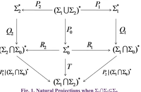
We employ the proposed method in [9] to investigate the observation properties in decentralized supervisory control (Fig.1). In general case, ⋃i≠j(Σi∩Σj)⊆Σ0, but for simplicity,
assume that Σ1∩Σ2⊆Σ0⊆Σ1∪Σ2, and the natural projections are defined as follows,
Pi:(Σ1∪Σ2)*⟶Σi* ,
Pi-1:Pwr(Σi*)⟶Pwr((Σ1∪Σ2)*), i=0,1,2
Qi: Σi*⟶(Σi∩Σ0)* ,
Qi-1:Pwr((Σi∩Σ0)*)⟶Pwr(Σi*), i=1,2 Ri: Σ0*⟶(Σi∩Σ0)* ,
Ri-1:Pwr((Σi∩Σ0)*)⟶Pwr(Σ0*), i=1,2
T: Σ0*⟶(Σ1∩Σ2)* , T-1:Pwr((Σ1∩Σ2)*)⟶Pwr(Σ0*).
It has been proved that if Σ1∩Σ2⊆Σ0, then P0(K1∥K2)=Q1 (K1)∥Q2(K2)=R1-1 Q1(K1)∩R2-1Q2(K2) [9]. Thus, we defined local observation properties in a distributed supervisory control [20].
4- 1- Local Normality
Normality is a observation property of a language, related to another language and a projection channel.
Based on normality definition, the supervisor K is (Lm (G),P)-normal, if synchronization of P(K) and Lm(G) is equal to that of K. We introduced a similar property for the decentralized (distributed) supervisory control.
In a decentralized supervisor, say Ki, the natural projection Qi
is defined as Qi: Σi*⟶(Σi∩Σ0)* and Qi(Ki) is the image of Ki.
If Qi(Ki) and Lm(G) is synchronized and the resulted language
is equal to Ki, then Ki is normal. Although, Ki is defined in
Σi*, Lm(G) is defined in Σ*. Thus, their reference sets must be the same.
Definition 1 (Local Normality)[20]: Let Ki be a language
for i=1,2 and Pi: Σ*⟶Σi*,Qi: Σi*⟶(Σi∩Σ0)*, i=1,2 and
Qi(s)=Qi(s`). Ki is called (Lm(G),Pi-1 ,Qi )-normal, if Pi-1Ki∩Lm(G)=Pi-1Qi-1QiKi∩Lm(G).
Also, K̅i is called (L(G),Pi-1,Qi)-Normal, if: Pi-1K̅i∩L(G)=Pi-1Qi-1QiK̅i∩L(G).
Comparing to the local normality, we call the normality global normality. In the following theorem, circumstances in which local and global normalities are equivalent are investigated. Theorem 1: Let Ki’s be control equivalent to K w.r.t. G
and observable events set be Σ0, such that Σ1∩Σ2⊆Σ0, Pi:(Σ1∪Σ2)*⟶Σi*,i=0,1,2, and Qj: Σj*⟶(Σj∩Σ0)*,j=1,2. Then local normality implies global normality and vice versa. Proof: (If) Let K1, K2 be two local normal languages. Then, P1-1K1∩Lm(G)=P1-1Q1-1Q1K1∩Lm(G),
P2-1K2∩Lm(G)=P2-1Q2-1Q2K2∩Lm(G).
Assume K1, K2 are control equivalent to K w.r.t. G. Thus,
K=P1-1K1∩P2-1K2∩Lm(G), We can write,
K=P1-1Q1-1Q1K1∩P2-1Q2-1Q2K2∩Lm(G). From Fig. 1 we have
Pi-1Qi-1=P0-1Ri-1 ,i=1,2 and
K=P0-1R1-1Q1K1∩P0-1R2-1Q2K2∩Lm(G).
From the properties of natural projection [9], we have P0-1(R1-1
Q1K1∩R2-1Q2K2)=P0-1R1-1Q1K1∩P0-1R2-1Q2K2 and P0K=R1-1
Q1K1∩R2-1Q2K2. Thus, K=P0-1P0(K)∩Lm(G). It means that K is (Lm(G), P0)-global normal language. With the same analysis
scenario, it can be proved that K̅ is (L(G),P0)-global normal if
both K̅i’s are (L(G),Pi-1 ,Qi)-local normal.
(Only if) Let K=P0-1P0(K)∩Lm(G) and the unobservable
events set be (Σ1∪Σ2)\Σ0. We assert that P1-1K1∩Lm(G)=P1-1
Q1-1Q1K1∩Lm(G) and P2-1K2∩Lm(G)=P2-1Q2-1Q2K2∩Lm(G). Assume P1-1K1∩Lm(G)≠P1-1Q1-1Q1K1∩Lm(G) or P2-1 K2∩Lm(G)≠P2-1Q2-1Q2K2∩Lm(G). Then,
P1-1Q1-1Q1K1∩P2-1Q2-1Q2K2∩Lm(G)⊈P1-1K1∩P2-1K2∩Lm(G) ⟹P0-1R1-1Q1K1∩P0-1R2-1Q2K2∩Lm(G)⊈K
⟹P0-1(R1-1Q1K1∩R2-1Q2K2 )∩L_m (G)⊈K ⟹P0-1P0(K)∩Lm(G)⊈K.
However, K=P0-1P0(K)∩Lm(G). Thus, by contradiction the claim is proved.
It is obvious the normality of a language is a strict condition. Hence, relative observability is more achievable than normality in practice.
4- 2- Local Relative Observability
Local relative observability was defined in [20] in the case of unobservable controllable events in decentralized supervisory control. This property makes a larger language than the supremal normal counterpart.
Definition 2 (Local Relative Observability)[20]: Let Ki be
a language for i=1,2 and K̅i⊆C̅i⊆PiL(G). Also, Pi: Σ*⟶Σi*,
Qi: Σi*⟶(Σi∩Σ0)* and Qi(s)=Qi(s`). Ki is locally relatively
observable w.r.t. (C̅i, G, Pi-1 ,Qi) if
(i``)(∀σ∈Σi) sσ∈K̅i ,s`∈C̅i, Pi-1(s`σ)∈L(G)⟹s`σ∈K̅i
(ii``) s∈Ki, s`∈C̅i, Pi-1(s`)∈Lm(G)⟹s`∈Ki.
According to Proposition 1, it is easy to show that the statements (i``) and (ii``) can be written as follows, respectively.
Pi-1Qi-1QiK̅i∩Pi-1C̅i Σ∩L(G)⊂Pi-1K̅i∩L(G), (11) Pi-1Qi-1QiKi∩Pi-1C̅i∩Lm(G)=Pi-1Ki∩Lm(G). (12) Proposition 6: Ki is locally relatively observable w.r.t. (C̅i, G, Pi-1 ,Qi) if and only if Qi(s)=Qi(s`) and (11), (12) hold.
Proof: This proposition is proved in the appendix.
Comparing to the local relative observability, we rename the relative observability global relative observability.
In the following proposition, some circumstances in which local and global relative observability are equivalent will be investigated.
Proposition 7: Let Ki’s be control equivalent to K w.r.t.
G, and observable event set be Σ0, which Σ1∩Σ2⊆Σ0 and Pi:(Σ1∪Σ2)*⟶Σi* ,i=0,1,2, Qj:Σj*⟶(Σj∩Σ0)*, j=1,2. Then local relative observability guarantees global relative observability, and global relative observability guarantees that at least one of the local controllers is locally relatively observable and the other is local normal.
Proof: This proposition is proved in the appendix.
If C̅i=K̅i, then local relative observability property turns into
local observability property. Thus, it is sufficient to replace C̅i
by K̅i in the local relative observability definition.
5- Observation-equivalent Versus Control Equivalent Previously, we showed that if all the shared events between local controllers (which are control equivalent to the monolithic supervisor w.r.t. the plant) are observable, then they have observation properties similar to those of the monolithic supervisor. For example, if K1, K2 are local controllers, and K
is relatively observable w.r.t. (C̅,G,P0), then K1, K2 are locally
relatively observable w.r.t. (C̅i, G, Pi-1, Qi) ,i=1,2 in the partial observation case. We prove that this property has an essential role to keep the local controllers control equivalent to the monolithic supervisor w.r.t. the plant.
Definition 3 (Observation-equivalent): Let K be a monolithic supervisor and Ki’s be local controllers with Pi:Σ*⟶Σi*
,i=0,1,2 and Qj:Σj*⟶(Σj∩Σ0)* ,j=1,2. Ki’s are observation equivalent to K w.r.t. G, if the following statement is satisfied. “∀i ,C̅i⊇K̅i, if Ki is locally relatively observable w.r.t. (C̅i,G, Pi-1 ,Qi), then ∃C̅⊇K̅ such that K is global relative observable
w.r.t. (C̅,G,P0).”
However, the control equivalency of a set of local controllers to the monolithic supervisor is guaranteed in full observation case; the observation equivalence of local controllers to the monolithic supervisor may be violated if the observation of local controllers is restricted to observe some events which are not significant for a consistent decision making. Hence, we investigate circumstances in which observation equivalence leads to the control equivalence.
In the following theorem, we prove that control equivalency
of local controllers to the monolithic supervisor is satisfied if and only if Σ1∩Σ2⊆Σ0.
Theorem 2: Let Ki’s be observation-equivalent to K w.r.t.
G, and observable events set be Σ0, where Pi:(Σ1∪Σ2)*⟶Σi*
,i=0,1,2, and Qj:Σj*⟶(Σj∩Σ0)*, j=1,2. Then, Ki’s are control
equivalent to K w.r.t. G if and only if Σ1∩Σ2⊆Σ0. Proof: (If) The proof is similar to that of Proposition 7. (Only if) Assume that Σ0⊆Σ1∩Σ2. Then, P1-1Q1-1=P2-1Q2-1=P0-1, P0K⊆Q1K1∩Q2K2 , and P1-1C̅1, P2-1C̅2 be in conflict. We can write,
P1-1K1∩P2-1K2∩Lm(G)=P1-1Q1-1Q1K1∩P2-1Q2-1Q2K2∩(P1-1
C̅1∩P2-1C̅2)∩Lm(G)=P0-1(Q1K1∩Q2K2)∩(P1-1C̅1∩P2-1
C̅2)∩Lm(G).
Define C≔P1-1C1∩P2-1C2. Then, C̅⊆P1-1C̅1∩P2-1C̅2. Thus, P0-1(P0K)∩C̅∩L(G)⊆P0-1(Q1K1∩Q2K2)∩P1-1C̅1∩P2-1
C̅2)∩L(G)⟹K⊆P1-1K1∩P2-1K2∩Lm(G). It means that K1 and K2 may be synchronously in conflict. By contradiction
Σ1∩Σ2⊆Σ0.
In Proposition 7, if K1 is locally observable w.r.t. (G, P1-1 ,Q1) (respectively K2 is local observable w.r.t.(G,P2-1) ,Q2)) then
C̅1=K̅1 (respectively C̅2=K̅2). Therefore, (C̅`≔P1-1C̅1∩P2-1
C̅2∩L(G)=P1-1 K̅1∩P2-1C̅2∩L(G) and K̅⊆C̅`. Namely, K is
globally relatively observable w.r.t. (C̅`,G,P0). Moreover, if K1 is locally normal w.r.t. (G,P1-1,Q1) then C̅``≔P1-1C̅1∩P2-1
C̅2∩L(G)=P2-1C̅2∩L(G) and K̅⊆C̅``. Namely, K is globally
relatively observable w.r.t. (C̅``,G,P0).
6- Examples
In this section, we consider four examples to illustrate the extended theorem in the previous sections.
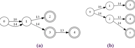
Example 1: Consider the plant G and the recognizer of the supervisor K given in Fig. 2. Assume that the set of all possible events is Σ={10,13,14}, the controllable events sets are Σ1,c=Σ2,c={13}, the observable events sets are Σ10={13,14}
and Σ20={13}, and the natural projections are as follows, Pi:Σ*⟶Σi* ,i=0,1,2, Qj: Σj*⟶Σj0* ,j=1,2
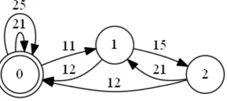
The local controllers which are control equivalent to the supervisor w.r.t. G are shown in Fig.3. The monolithic supervisor and local controllers are constructed by TCT software [25]. Synchronization of local controllers with the plant is the same as that of the monolithic supervisor, shown in Fig. 2 (b). Fig. 4 shows the recognizer of the monolithic supervisor with partial observation. K is globally relatively observable w.r.t. (C̅,G,P0), where C̅={10,1014,101413,14,1 413,1414}⊆L(G). Fig. 5 shows local controller 1 with full observation and local controller 2 with partial observation. Also, the synchronization of local controllers (Fig.5) and the plant is control equivalent to the monolithic supervisor with a partial observation (Fig. 4).
Therefore, when event {10} is not observable for the monolithic supervisor, it can be unobservable for local controller 2, whereas control equivalency between local controllers and
(a) (b)
(b) (a)
(a) (b)
Fig. 3. Local controllers with full observation, (a) Local
controller1 with full observation Σ1={13,14} , (b) Local
controller 2 with full observation Σ2={10,13}
Fig. 8. Local relative observable controller for M1
Fig. 9. Local normal controllers for M2 and TU
Fig. 10. Schematic of a guide way
Fig. 11. Discrete-event model of vehicles V1,V2
Fig. 12. Recognizer of the supremal normal supervisor (K)
Fig. 13. Recognizer of the reduced supremal normal supervisor Fig. 4. Recognizer of the monolithic supervisor K with partial
observation, Σ0={13,14}
Fig. 5. Local controllers with partial observation Σ0={13,14}
, (a) Local controller1 with full observation Σ10={13,14} , (b)
Local controller2 with partial observation Σ20={13}
Fig. 6. Transfer Line
the monolithic supervisor w.r.t. G is preserved. This raises the concept of observation equivalency. It means that, if local controller 2, that is shown in Fig.5 (b), has conflict with the other local controller, then their synchronization with the plant is not control equivalent to the monolithic supervisor (shown in Fig. 4) w.r.t. G.
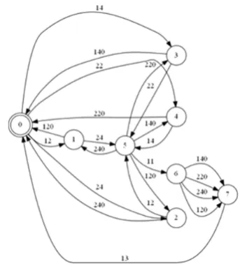
Example 2 (Supremal relative observable supervisor for Transfer Line): Industrial Transfer Line is a simple model of industrial systems and consists of two machines M1, M2 and a test unit (TU), such that they are linked by buffers B1 and B2 with the capacity of three and one slots, respectively (Fig. 6). If a work piece accepted by TU, it is released from the system; if it is rejected, then it is returned to B1 for reprocessing by M2. The control logic is based on protection B1 and B2 against underflow and overflow [24]. Controllable events are odd-numbered and the unobservable event is {1}. Fig.7 shows the reduced supremal relative observable supervisor synthesized by TCT software [25]. Local controller for the component M1 is shown in Fig. 8 and for M2 and TU in Fig. 9. The local controller of M1 is locally relatively observable and the local controllers of M2 and TU are locally normal. If event {1} is unobservable for local controller of M1, then it becomes self-looped at all states of the local controller (it is not shown). The local controllers of M2 and TU are locally normal because event {1} is self-looped at all states as shown Fig. 9. It means that event {1} does not affect local controllers of M2 and TU, even they are under full observation or under partial observation.
It can be interpreted that event {1} does not belong to local controllers of M2 and TU. Therefore, the global relative observability of the monolithic supervisor leads to the local relative observability of local controller M1 and leads to local normality of local controllers M2 and TU.
Example 3(Supremal normal supervisor for a Guide way) On a typical guide way, stations A and B are connected by a one-way track from A to B, as shown in Fig. 10. The track consists of four sections, with stoplights which are shown with (*) and with detectors which are shown by (!), installed at various section junctions [23].
Two vehicles V1 and V2 use the guide way simultaneously. Vi ,i=1,2, may be at state 0 (at A), state j (while travelling in
section j=1,….,4), or state 5 (at B). The discrete-event models of Vi ,i=1,2 are shown in Fig. 11.
The plant to be controlled is G=sync(V1,V2). In order to prevent collision, control of the stoplights must ensure that V1 and V2 never travel on the same section of the track, simultaneously. In this example, unobservable events are {13,23}. Fig. 12 shows the recognizer of the supremal normal supervisor, and Fig.13 shows the recognizer of the reduced supervisor in which unobservable events {13,23} are not shown, i.e. they are self-looped at all states in the reduced supervisor.
Events {13,23} belong to null space of an arbitrary natural projection P as follows,
P:Σ*→Σ
0* ,Σ0=Σ−{13,23}
The local normal controllers for components V1 and V2, are shown in Fig. 14 and Fig. 15. They are locally normal; because local controllers do not regard the events {13,23}. Therefore, the global normality leads to local normality and vice versa.
Example 4 (Supervisory control synthesis for balancing the pressure of parallel gas trunk lines)
The main sector of a long-distance gas transmission system
is a gas trunk line. A gas trunk line is a pipeline which is designed for natural gas transmission from production to market areas. It is similar to trunk of a tree in which the gas processing plants deliver the natural gas through several roots, and consumers receive the gas from some branches. Natural gas is pressurized so that it travels through a pipeline to transport the flow of gas. To keep the minimum pressure for flowing natural gas through each pipeline, compression of the natural gas occurs periodically along the pipe. This is accomplished by compressor stations, placed according to the land topography along the pipeline. Natural gas pipelines include a great number of valves along their entire length. They are divided into two categories: 1. Line Break Valves (LBV’s), usually open and allow natural gas to flow freely, but they can be used to stop gas flow along a section of pipe. There are many reasons why a pipeline may need to restrict gas flow in certain circumstances, namely emergency shutdown and maintenance. 2. Control Valves placed on connection pipes between two trunk lines. They are called connection valves each of which connects two trunk lines through a certain connection line.
Since the consumption of natural gas shall be distributed across the trunk lines, several branches from a trunk line are taken to provide the consumption. Hence, the pressure of each trunk line may fluctuate by gas consumption throughout a trunk line. In order to balance the pressure of two or more parallel gas trunk lines, each connection valve between a pair of trunk lines segments can be set to open (Figs. 16, 17, 18). The supervisory control problem for a discrete-event system is formulated by modeling the plant and its control logic (specification) as finite automata [24].
The discrete-event modeling of parallel gas trunk lines, description of specifications, supervisor synthesis and state reduction of the supervisor is carried out in TCT software [25]. We construct a DES model for each pair of parallel gas trunk lines and associated connection valves as follows,
PVij= Sync(Pi, Pj, Vi) (18, 66) Blocked_events = None Pi, Pj and Vi are DES models of each pair of parallel gas trunk lines and the connection valve which is placed on the connection pipe between the two trunk lines (Fig. 19). PVij has 18 states and 66 transitions. Each pair of parallel trunk lines has the same structure with different events.
The control logic for opening and closing the valve is designed as several “If-Then” rules in Table 1, and the corresponding DES model is shown in Fig. 20. It is provided by a designer for balancing the pressure of two parallel gas trunk lines 1 and 2. The continuous time dynamics of the pressures in a segment of trunk lines 1 and 2, influenced by open/close actuations of the connection valve (Fig. 16) is shown in Fig. 21. The minimum
and the maximum permissible pressures are assumed to be 50 bar and 60 bar, respectively for each trunk line. Dashed lines show the variations of pressures in one segment of trunk lines 1 and 2, influenced by inlet and outlet gas flows (Fig. 21). This simulation is carried out by state flow toolbox in Matlab. In the case of three parallel gas trunk lines, we obtain two other control logics, structurally the same as E1 with different events for the other two pairs of parallel trunk lines (2,3) and (1,3). Each decentralized supervisor can be synthesized using supcon procedure as follows,
SUPij = Supcon (PVij, Ei) (34,95)
Each decentralized supervisor has 34 states and 95 transitions. We can show that SUP12, SUP23 and SUP13 are synchronously non-conflicting. Now, assume that events {11,21} are Fig. 19. DES model for each trunk line and the connection
valve, i=1,2,3
(a) Trunk Lines (Pi), (b) Connection Valve (Vi) Fig. 16. Schematic diagram of a supervisory control for two
parallel gas trunk lines
Fig. 17. Schematic diagram of a Monolithic (centralized) supervisory control for three parallel gas trunk lines
Fig. 20. DES model of the specification for balancing the pressure of two parallel gas trunk lines, E1
Table 1. Specifications as “If-Then” rules
Fig. 18. Schematic diagram of decentralized supervisory control for three parallel gas trunk lines
(a)
(b)
Rule
no. If Then
1
The connection valve is closed- ev .13, and the pressure of trunk line
1 is Low- ev.14 (High- ev.12), and the pressure of trunk line 2 is
High- ev.22 (Low- ev.24)
Open the connection valve (ev.11)
2
The connection valve is open- ev.11 and the pressure of trunk line 1 returns to the permissible
range (from min.)- ev.140
Close the connection valve (ev.13)
3
The connection valve is open- ev.11 and the pressure of trunk line 1 returns to the permissible
range (from max.)- ev.120
Close the connection valve (ev.13)
4
The connection valve is open- ev.11 and the pressure of trunk line 2 returns to the permissible
range (from min.)- ev.240
Close the connection valve (ev.13)
5
The connection valve is open- ev.11 and the pressure of trunk line 2 returns to the permissible
range (from max.)- ev.220
unobservable. Two supremal relative observable supervisors ROSUP12 and ROSUP23 can be synthesized using supconrobs procedure as follows,
ROSUP12= Supconrobs(PV12, E1, Null[11]) (65, 181) ROSUP23= Supconrobs(PV23, E2, Null[21]) (65, 181) Moreover,
SUP13 = Supcon(PV13, E3) (34,95)
SUP13 is synthesized based on full observation of PV13. The desired behavior (specification) of three parallel gas trunk lines can be obtained as follows,
E= Meet(E1, E2, E3) (512, 6528)
Assume controllable events {11,21} are unobservable. The supremal relative observable monolithic supervisor can be synthesized by supconrobs procedure as follows,
ROSUP= Supconrobs(PLANT, E, Null[11,21]) (1648, 7272) ROSUP is the relative observable supervisor with 1648 states and 7272 transitions.
On the other hand, the conjunctive behavior of ROSUP12, ROSUP23 and SUP13, can be obtained as follows,
SROSUP12= Selfloop (ROSUP12, [32, 34, 320, 340, 21, 23, 31, 33]) (65,367)
SROSUP23= Selfloop(ROSUP23, [12, 14, 120, 140, 11, 13, 31, 33]) (65,367)
SSUP13= Selfloop(SUP23, [12, 14, 120, 140, 11, 13, 21, 23]) (34,367)
DSUP = Meet(SROSUP12, SROSUP23, SSUP13) (1648, 7272) We can check the identity of DSUP and ROSUP by isomorph procedure.
true = Isomorph(DSUP, ROSUP; identity)
Since unobservable events {11,21} are not the shared events, local relative observability of decentralized supervisors leads to global relative observability of the monolithic supervisor (ROSUP).
In this example, we clarified that local observation properties lead to the global ones, if the shared events are observable. We know that decentralized supervisory controllers may be in conflict with each other because each decentralized supervisor observes the plant partially. The extended theory in this paper implies that, if the shared events of decentralized supervisors are observable, then unobservable events, in a relative observable supervisor, do not cause the conflict in the plant. In this example {11, 21} are unshared events.
7- CONCLUSIONS
In this paper, a method was introduced to analyze the observation properties such as relative observability, in a set algebra approach . Moreover, the observation properties in distributed supervisory control were investigated. We proved that with having local controllers and the monolithic supervisor, the partial observation properties are preserved from the global supervisor to the local controllers if and only if the intersection of local event sets is a subset of or equal to the global observable event set. Furthermore, the concept of control equivalency was extended for observation problem. Observation equivalence describes the equivalency of observations in the local controllers and the monolithic supervisor in order to have equivalency between control behavior in the monolithic and distributed supervisory control of the plant. It was proved that with having equivalency between local controllers and the monolithic supervisor, the control equivalency is satisfied if and only if the intersection of local event sets is a subset of or equal to the globally
observable event set. The extended theory was illustrated by four examples.
Appendix 1
In this appendix, we prove some propositions mentioned in this paper.
Proof of Proposition 2: We have P-1PK̅∩C̅Σ∩L(G)⊂K̅,
P-1PK∩C̅∩L m(G)=K. Then,
P-1PK̅∩C̅Σ∩L(G)∩K̅Σ⊂K̅∩K̅Σ, P-1PK∩C̅∩L
m(G)∩K̅=K∩K̅. On the other hand,
K̅⊆C̅ ⟹ K̅Σ⊆C̅Σ. Thus,
P-1PK̅∩K̅Σ∩L(G)⊂K̅, P-1PK∩K̅∩L
m(G)=K. Therefore, K is observable. Proof of Proposition 3: We have P-1PK̅∩L(G)=K̅,
a. Variations in pressure of trunk line 1, influenced by open/ close actuations in the connection valve
b. Variations in pressure of trunk line 2, influenced by open/ close actuations in the connection valve
P-1PK∩L
m(G)=K. Then,
P-1PK̅∩L(G)∩C̅Σ=K̅∩C̅Σ, P-1PK∩L
m(G)∩C̅=K∩C̅.
Also K⊆K̅⊆C̅ and K̅∩C̅Σ⊂K̅. Thus, P-1PK̅∩L(G)∩C̅Σ⊂K̅,
P-1PK∩L
m(G)∩C̅=K.
Proof of Proposition 4: Assume that P-1PK̅
i∩C̅Σ∩L(G)⊂K̅i, P-1PK
i∩C̅∩Lm(G)=Ki. We can write
⋃i{P-1PK̅i∩C̅Σ∩L(G)}⊂⋃iK̅i , ⋃i{P-1PKi∩C̅∩Lm(G)}=⋃iKi . Thus,
⋃i{P-1PK̅i}∩C̅Σ∩L(G)⊂⋃iK̅i , ⋃i{P-1PKi}∩C̅∩Lm(G)=⋃iKi .
From the properties of natural projection [9], it holds that P-1P(⋃
i{K̅i})∩C̅Σ∩L(G)⊂⋃iK̅i , P-1P(⋃
i{Ki})∩C̅∩Lm(G)=⋃iKi . Therefore,
P-1PK̅∩C̅Σ∩L(G)⊂K̅, P-1PK∩C̅∩L
m(G)=K.
Proof of Proposition 5: Assume that P-1PK̅
i∩C̅Σ∩L(G)⊂K̅i, P-1PK
i∩C̅∩Lm(G)=Ki. Then,
⋂i{P-1PK̅i∩C̅Σ∩L(G)}⊂⋂iK̅i , ⋂i{P-1PKi∩C̅∩Lm(G)}=⋂iKi .
From the properties of natural projection [9], ⋂i{P-1PKi}∩C̅∩Lm(G)⊆P-1P{⋂iKi}∩C̅∩Lm(G). Thus,
⋂iKi⊆P-1P{⋂iKi}∩C̅∩Lm(G).
Let K=⋂iKi . We can write K⊆P-1P{K}∩C̅∩Lm(G).
Therefore, the closeness of relative observability, under intersection, is not guaranteed.
Proof of Proposition 6: (If) Assume Q_i (s)=Q_i (s^’) and (11), (12) do hold. We can write,
(∀σ∈Σi) sσ∈K̅i ,s`∈C̅i,Pi-1(s`σ)∈L(G)⟹s`σ∈C̅i Σi. Also,
Qi(s)=Qi(s`)⟹Qi(sσ)=Qi(s`σ)⟹s`σ∈Qi-1Qi K̅i ⟹Pi-1(s`σ)∈Pi-1Qi-1Qi K̅i∩Pi-1C̅i Σ∩L(G). From (11), we can write
⟹Pi-1(s`σ)∈Pi-1K̅i∩L(G)⟹s`σ∈K̅i∩Pi L(G) ⟹s`σ∈K̅i.
Thus, (i``) is proved. From (12), we can write,
s∈Ki,s`∈C̅i,Pi-1(s`)∈Lm(G)⟹Pi-1(s`)∈Pi-1C̅i. Also,
Qi(s)=Qi(s`)⟹s`∈Qi-1QiK̅i⟹Pi-1(s`)∈Pi-1Qi-1QiK̅i ⟹Pi-1(s`)∈Pi-1Qi-1Qi Ki∩Pi-1C̅i∩Lm(G).
From (12), we can write, ⟹Pi-1(s`)∈Pi-1Ki∩Lm(G) ⟹s`∈Ki∩Pi Lm(G) ⟹s`∈Ki.
Thus, (ii``) is proved.
(Only if) Assume Qi(s)=Qi(s`) and (i``) hold. we can write
sσ∈K̅i ,s`∈C̅i, Pi-1(s` σ)∈L(G)⟹s` σ∈K̅i
⟹Qi(sσ)∈QiK̅i ,s`∈C̅i, Pi-1(s` σ)∈L(G)⟹s` σ∈K̅i ⟹Qi(s`σ)∈QiK̅i ,s`∈C̅i, Pi-1(s` σ)∈L(G)⟹s` σ∈K̅i ⟹s`σ∈Qi-1QiK̅i ,s`∈C̅i,Pi-1(s`σ)∈L(G)⟹s`σ∈K̅i
⟹Pi-1(s`σ)∈Pi-1Qi-1QiK̅i ,Pi-1(s`σ)∈Pi-1C̅iΣ, Pi-1(s`σ)∈L(G) ⟹s`σ∈K̅i ⟹Pi-1(s`σ)∈Pi-1K̅i,Pi-1(s`σ)∈L(G)
⟹Pi-1Qi-1QiK̅i∩Pi-1C̅iΣ∩L(G)⊆Pi-1K̅i∩L(G). On the other hand,
ϵ∉Pi-1C̅i Σ,ϵ∈Pi-1K̅i ⟹
Pi-1Qi-1QiK̅i∩Pi-1C̅iΣ∩L(G)⊂Pi-1K̅i∩L(G).
Moreover, (i``) holds. Then, s∈Ki,s`∈C̅i,Pi-1(s`)∈Lm(G)⟹s`∈Ki
⟹Qi(s)∈Qi Ki ,s`∈C̅i,Pi-1(s`)∈Lm(G)⟹s`∈Ki ⟹Qi(s`)∈QiKi,s`∈C̅i,Pi-1(s`)∈Lm(G)⟹s`∈Ki ⟹s`∈Qi-1Qi Ki ,s`∈C̅i,Pi-1(s`)∈Lm(G)⟹s`∈Ki ⟹Pi-1(s`)∈Pi-1Qi-1QiKi ,Pi-1(s`)∈Pi-1C̅i,Pi-1(s`)∈Lm(G) ⟹s`∈Ki⟹Pi-1(s`)∈Pi-1Ki,Pi-1(s`)∈Lm(G)
⟹Pi-1Qi-1QiKi∩Pi-1C̅i∩Lm(G)⊆Pi-1Ki∩Lm(G).
Moreover, Pi-1Ki⊆Pi-1C̅i and Pi-1Ki⊆Pi-1Qi-1QiKi hold. Thus, Pi -1K
i∩Lm(G)⊆Pi-1Qi-1QiKi∩Pi-1C̅i∩Lm(G). Therefore, we can write
Pi-1Qi-1QiKi∩Pi-1C̅i∩Lm(G)=Pi-1Ki∩Lm(G).
Proof of Proposition 7: (If) Let K1, K2 be two locally relatively observable languages. We can write,
P1-1Q1-1Q1K̅1∩P1-1C̅1Σ∩L(G)⊂P1-1K̅1∩L(G), P2-1Q2-1Q2K̅2∩P2-1C̅2Σ∩L(G)⊂P2-1K̅2∩L(G).
We have K1, K2 which are control equivalent to K w.r.t.G. Thus,
K̅=P1-1K̅1∩P2-1K̅2∩L(G),
⟹P1-1Q1-1Q1K̅1∩P2-1Q2-1Q2K̅2∩(P1-1)C̅1∩P2-1C̅2)Σ∩L(G)⊂K̅.
By defining C̅∶=P1-1C̅1∩P2-1C̅2∩L(G), we have K̅⊆C̅⊆L(G), and P0-1R1-1Q1K̅1∩P0-1R2-1Q2K̅2∩C̅Σ∩L(G)⊂P0-1R1-1 Q1K̅1∩ P0-1 R2-1Q2K̅2∩(P1-1C̅1∩P2-1C̅2)Σ∩L(G). Thus, P0-1(P0K̅)∩C̅Σ
∩L(G)⊂K̅.
Similarly, it can be proved that K=P0-1(P0K)∩C̅∩Lm(G).
Therefore, K is (C̅,G,P0)-global relative observable.
(Only if) Let P0-1(P0K̅)∩C̅Σ∩L(G)⊂K̅ ,K̅⊆C̅⊆L(G), and
relativey observable. Thus, P0-1(P0K̅)∩C̅Σ∩L(G)⊂K̅
⟹P0-1(R1-1Q1K̅1∩R2-1Q2K̅2)∩C̅Σ∩L(G)⊂K̅ ⟹P0-1R1-1Q1K̅1∩P0-1R2-1Q2K̅2∩C̅Σ∩L(G)⊂K̅.
We claim that there exists K̅1⊆C̅1, where P1-1Q1-1Q1 K̅1∩P1-1
C̅1Σ∩L(G)⊂P1-1K̅1∩L(G) and K̅2⊆C̅2, where P2-1Q2-1Q2K̅2∩P2-1
C̅2Σ∩L(G)⊂P2-1 K̅2∩L(G) (or P2-1Q2-1Q2 K̅2∩L(G)=P2-1
K̅2∩L(G)). Otherwise,
P1-1K̅1∩L(G)⊆P1-1 Q1-1Q1K̅1∩P1-1C̅1Σ∩L(G), (13) or
P2-1K̅2∩L(G)⊆P2-1Q2-1Q2K̅2∩P2-1C̅2Σ∩L(G). (14)
If both (13), (14) are satisfied, then K̅=P1-1K̅1∩P2-1
K̅2∩L(G)⊆P0-1P0K̅∩C̅Σ∩L(G); But P0-1P0K̅∩C̅Σ∩L(G)⊂K̅. If only one of the two relationships (13) or (14) holds, then Q1-1Q1=Q2-1Q2=1. It means that the projection channels
Qi ,i=1,2 allow passing all the events from their reference events set. By contradiction, there should be P1-1Q1-1
Q1K̅1∩P1-1C̅1Σ∩L(G)⊂P1-1K̅1∩L(G) and P2-1 Q2-1 Q2K̅2∩P2-1
C̅2Σ∩L(G)⊂P2-1K̅2∩L(G). Furthermore, it is easy to prove that if one of the local controllers is locally relatively observable and the other one is locally normal, then K is globally relatively observable. The following relationships can be proved, similarly.
P1-1K1∩Lm(G)=P1-1Q1-1Q1K1∩P1-1C̅1∩Lm(G), P2-1K2∩Lm(G)=P2-1Q2-1Q2K2∩P2-1C̅2∩Lm(G).
Appendix 2
A quick review of TCT commands is presented.
DES3=supcon(DES1, DES2) for a controlled generator DES1, forms a trim recognizer for the supremal controllable sublanguage of the marked (“legal”) language generated by DES2 to create DES3. This structure provides a proper supervisor for DES1.
DES = sync(DES1,DES2,: : : ,DESk)
is the (reachable) synchronous product of DES1,DES2,: : : ,DESk.
DAT3= condat(DES1, DES2) returns control data DAT3 for the supervisor DES2 of the controlled system DES1. If DES2 represents a controllable language (with respect to DES1),as when DES2 has been previously computed with supcon, then condat will display the events that are disabled at each state of DES2. In general, condat can be used to test whether a given language DES2 is controllable: just check that the disabled events tabled by condat are themselves controllable (have odd-numbered labels).
DES3=supreduce(DES1, DES2, DAT2) is a reduced supervisor for plant DES1 which is control-equivalent to DES2, where DES2 and control data DAT2 were previously computed using supcon and condat. Also, returned is an estimated lower bound slb for the state size of a strictly state-minimal reduced supervisor. DES3 is strictly state-minimal if its reported state size equals the slb.
{LOC1,LOC2,...,LOCm} = localize(PLANT,{PLANT1,… ,PLANTm},SUPER)is the set of localizations of SUPER to the m independent components PLANT1,...,PLANTm of PLANT. Independence means that the alphabets
of PLANT1,...,PLANTm must be pair wise disjoint. Optionally, correctness of localization is verified and reported as ControlEqu(...). Localize is mainly for use when SUPER is a decentralized supervisor with authority over PLANT1,...,PLANTm, and PLANT is their synchronous product.
DES2=project(DES1, NULL/IMAGE EVENTS) is a generator of the projected closed and marked languages of DES1, under the natural projection specified by the listed Null or Image events.
True/False= isomorph(DES1, DES2) tests whether DES1 and DES2 are identical up to renumbering of states; if so, their state correspondence is displayed.
REFERENCES
[1] P.J. Ramadge, W.M. Wonham, Supervisory control of a class of discrete event processes, SIAM journal on control and optimization, 25(1) (1987) 206-230.
[2] F. Lin, W.M. Wonham, Decentralized control and coordination of discrete-event systems with partial observation, IEEE Transactions on automatic control, 35(12) (1990) 1330-1337.
[3] J. Komenda, J.H. van Schuppen, Modular control of discrete-event systems with coalgebra, IEEE Transactions on Automatic Control, 53(2) (2008) 447-460.
[4] H. Zhong, W.M. Wonham, On the consistency of hierarchical supervision in discrete-event systems, IEEE Transactions on automatic Control, 35(10) (1990) 1125-1134.
[5] K.C. Wong, W.M. Wonham, Hierarchical control of discrete-event systems, Discrete Event Dynamic Systems, 6(3) (1996) 241-273.
[6] K.C. Wong, W.M. Wonham, Modular control and coordination of discrete-event systems, Discrete Event Dynamic Systems, 8(3) (1998) 247-297.
[7] K. Schmidt, T. Moor, S. Perk, Nonblocking hierarchical control of decentralized discrete event systems, IEEE Transactions on Automatic Control, 53(10) (2008) 2252-2265.
[8] K. Schmidt, C. Breindl, Maximally permissive hierarchical control of decentralized discrete event systems, IEEE Transactions on Automatic Control, 56(4) (2011) 723-737.
[9] L. Feng, W.M. Wonham, Supervisory control architecture for discrete-event systems, IEEE Transactions on Automatic Control, 53(6) (2008) 1449-1461.
[10] T.-S. Yoo, S. Lafortune, A general architecture for decentralized supervisory control of discrete-event systems, Discrete Event Dynamic Systems, 12(3) (2002) 335-377.
[11] K. Rudie, W.M. Wonham, Think globally, act locally: Decentralized supervisory control, IEEE transactions on automatic control, 37(11) (1992) 1692-1708.
[12] K. Cai, R. Zhang, W.M. Wonham, On relative observability of discrete-event systems, in: Decision and Control (CDC), 2013 IEEE 52nd Annual Conference on, IEEE, 2013, pp. 7285-7290.
[14] J. Komenda, T. Masopust, J.H. van Schuppen, On conditional decomposability, Systems & Control Letters, 61(12) (2012) 1260-1268.
[15] K. Cai, W.M. Wonham, Supervisor localization: a top-down approach to distributed control of discrete-event systems, IEEE Transactions on Automatic Control, 55(3) (2010) 605-618.
[16] F. Lin, W.M. Wonham, On observability of discrete-event systems, Information sciences, 44(3) (1988) 173-198. [17] K. Cai, R. Zhang, W.M. Wonham, Relative observability
of discrete-event systems and its supremal sublanguages, IEEE Transactions on Automatic Control, 60(3) (2015) 659-670.
[18] E. José, N. Patrícia, L. Stéphane, Verification of Nonconflict of Supervisors Using Abstractions, (2009). [19] R. Zhang, K. Cai, W.M. Wonham, Supervisor
localization of discrete-event systems under partial observation, Automatica, 81 (2017) 142-147.
[20] V. Saeidi, A.A. Afzalian, D. Gharavian, Distributed supervisory control with partial observation, in: Control, Instrumentation, and Automation (ICCIA), 2016 4th International Conference on, IEEE, 2016, pp. 136-141.
[21] S. Mohajerani, R. Malik, M. Fabian, An algorithm for weak synthesis observation equivalence for compositional supervisor synthesis, IFAC Proceedings Volumes, 45(29) (2012) 239-244.
[22] M. Noorbakshsh, A. Afzalian, Design and PLC based implementation of supervisory control for under-load tap-changing transformers, in: Control, Automation and Systems, 2007. ICCAS’07. International Conference on, IEEE, 2007, pp. 901-906.
[23] A. Afzalian, A. Saadatpoor, W. Wonham, Systematic supervisory control solutions for under-load tap-changing transformers, Control Engineering Practice, 16(9) (2008) 1035-1054.
[24] R. Zhang, K. Cai, Y. Gan, W.M. Wonham, Distributed supervisory control of discrete-event systems with communication delay, Discrete Event Dynamic Systems, 26(2) (2016) 263-293.
[25] W. Wonham, Control design software: TCT, Developed by Systems Control Group, Univ. Toronto. Toronto, Canada, (2014).
Please cite this article using:
V. Saeidi, A. Afzalian, D. Gharavian, Partial Observation in Distributed Supervisory Control of Discrete-Event Systems, AUT J. Model. Simul., 49(2)(2017)187-198.