Towards Model-checking Probabilistic Timed
Automata against Probabilistic Duration Properties
I
Van Hung Dang
1,∗, Miaomiao Zhang
2, Dinh Chinh Pham
1 1VNU University of Engineering and Technology, Hanoi, Vietnam 2School of Software Engineering, Tongji University, Shanghai, ChinaAbstract
In this paper, we consider a subclass of Probabilistic Duration Calculus formula called Simple Probabilistic Duration Calculus (SPDC) as a language for specifying dependability requirements for real-time systems, and address the two problems: to decide if a probabilistic timed automaton satisfies a SPDC formula, and to decide if there exists a strategy of a probabilistic timed automaton satisfies a SPDC formula. We prove that the both problems are decidable for a class of SPDC called probabilistic linear duration invariants, and provide model checking algorithms for solving these problems.
Received 25 November 2015, revised 20 December 2015, accepted 31 December 2015
Keywords: Probabilistic Duration Calculus, Probabilistic Timed Automata, Model-checking, Markov Decision Process.
1. Introduction
In 1992, Chaochen Zhou, Hoare C.A.R and Anders Ravn introduced Duration Calculus [1] as a logic for reasoning about real-time systems. The calculus has attracted a great deal of attention, and was then developed further in many other works because of its rich meanings. Many of those works have been summarized
in the monograph [2]. For specifying the
dependability of real-time systems, a kind of probabilistic extension of Duration Calculus has been introduced in [3, 4]. No rigorous syntax has been introduced in these papers, and the authors just focused on the development of techniques for reasoning instead of the ones for checking. A version with a proof system of Probabilistic Duration Calculus with infinite interval was then
IThis research was funded by Vietnam National Foundation
for Science and Technology Development (NAFOSTED) under grant number 102.03-2014.23.
∗
Corresponding author. Email: [email protected]
developed by Dimitar Guelev [5], and in [6] we have shown that the calculus is useful for reasoning about QoS contracts in component-based real-time systems.
For Duration Calculus, some techniques for checking if a timed automaton satisfies a duration calculus formula written in the form of linear duration invariants have been developed [7, 8,
9, 10, 11, 8]. However, to our knowledge,
not many works have been done for checking if a probabilistic real-time system satisfies a
PDC formula. This is, perhaps, because in
the model of probabilistic systems, there is too much randomization and nondeterminism, and this makes model checking too complicated.
Kwiatkowska et al in [12, 13] proposed a variant of probabilistic timed automata that allows probabilistic choice only at discrete
transitions. To resolve the nondeterminism
between the passage of time and discrete transitions they used the concept of strategy which is essentially a deterministic schedule
policy. Then, the set of executions of a probabilistic timed automaton according to a strategy forms a Markov chain, and hence the satisfaction of a probabilistic timed CTL formula by this set can be defined, and then based on the region graph of the timed automaton the satisfaction of a probabilistic timed CTL formula by the timed automaton can be also verified. The idea of fixing a strategy when studying the probabilistic behavior of a probabilistic timed automaton restricts the scope of the verification
problem significantly, making the checking
problem more tractable. Then, verifying the
set of all strategies against a given probabilistic property can be done by searching for the “worst case” strategy according to the probabilistic property and then apply the verification technique to it. This idea is a motivation for us to reconsider
the problem of checking a probabilistic
timed automaton for a PDC formula that we gave up before.
In this paper, we introduced a simple
probabilistic extension of DC called Probabilistic Duration Calculus for specifying dependability requirements of real-time systems. The extension is conservative in the sense that a formula of DC is also a formula of PDC with semantics
adapted to probabilistic domain. PDC also
consists of formulas representing the constraints for the probability of the satisfaction of a DC formula by a strategy for an interval. We use the behavioral model proposed by Kwiatkowska et al to define the semantics of
our logic. Since probabilistic timed CTL and
PDC are not comparable, and since for many probabilistic properties PDC is more convenient to specify, a model checking technique for checking probabilistic timed automata against PDC properties is useful. To solve this problem, we first develop a technique to decide if a strategy in a probabilistic timed automaton satisfies a PDC formula of a certain form. This technique is essentially an extension of our technique developed earlier in [10, 9] to check if a timed automaton satisfies a DC formula in the form of linear duration invariants or discretisable DC formulas based on searching in the integral
reachability graph of the timed automaton. Then, we generalize this technique to achieve our goal with a model-checking algorithm.
The first version of this paper was published in [14]. In this extended version, in addition to the problem of verification, we formulate also the problem of strategy synthesis, i.e. to decide if there is a strategy for a probabilistic timed automaton that satisfies a probabilistic linear duration invariant and show that this problem is also solvable. We provide all proof details and algorithms for doing model-check.
Our paper is organized as follows. In the
next section we present the Probabilistic Timed
Automata model. Section 3 presents syntax
and semantics of our PDC. Our main results is presented in Section 4 where we formulate our model checking problem and give our solution to it. The last section is the conclusion of the paper.
2. Probabilistic Timed Automata
In this section, we recall the concepts
of probabilistic timed automata model and probabilistic timed structure as its semantics
from [15, 12]. We use a simple model of
gas burners to illustrate the concepts as its requirement specification is a typical example for time duration properties.
Probability distributions and Markov decision processes. A discrete probability distribution
over a set S is a mapping p : S → [0,1] such
that the set{s| s ∈S andp(s) > 0}is finite, and
P
s∈S p(s)= 1. The set of all discrete probability distributions overS is denoted byµ(S).
A Markov decision process is a tuple
(Q,Steps), where Q is a set of states, and
Steps : Q → 2µ(Q) is a function assigning a set of probability distributions to each state. The intuition is that the Markov decision process traverses the state space by making transitions determined bySteps: in a state s, the process selects nondeterministically a probability
distribution p in Steps(s), and then makes a
probabilistic choice according to p as to which
fromΣ, and assume thatSteps:Q →2Σ×µ(Q)and
Σis a set of actions. The intuition now becomes
that the Markov decision process traverses the state space by making transitions determined by
Steps: in a state s, the process performs an
action a ∈ Σ selecting nondeterministically a
probability distribution p in Steps(s), and then
makes a probabilistic choice according to pas to
which state to move to. So, a transition is of the form s −→a,p s0, where (a,p) ∈ Σ× µ(Q) is the label of the transition. We also assume a labeling
function L : Q → 2AP, where AP is a set of
atomic propositions, that associates a stateswith the set of atomic propositions that hold at state
s. Then, a labeled Markov decision process is
a tuple (Q,Steps,L).
Labeled paths (or execution sequences)
are nonempty finite or infinite sequence of consecutive transitions of the form
ω = s0
l0
−→s1
l1
−→ s2
l2
−→. . . ,
wheresiare states andliare labels for transitions. For a path ω, let f irst(ω) denote the first state of ω, and if ω is finite then let last(ω) denote the last state of ω. |ω| is the length ofω and is defined as the number of transition occurrences
in ω which is ∞ if ω is infinite. For k ≤ |ω|,
let ω(k) denote thekth state ofω, andstep(ω,k) denote the label of the kth transition inω. For
two paths ω = s0
l0
−→ s1
l1
−→ s2
l2
−→ . . .sn and ω0 = s00
l00 −→ s01
l01 −→ s02
l02
−→ . . . such that
sn = s00, the concatenation ofωandω0is defined asωω0 = s0
l0
−→ s1
l1
−→ s2
l2
−→. . .sn l00 −→ s01
l01 −→
s02
l0 2
−→. . ..
Clocks, clock valuations, clock constraints.Let
R≥0denote the set of non negative real numbers.
A clock is a real-valued variable which increases at the same rate as real time. LetC={x1. . . ,xn} be a set of clocks. A clock valuation is a function
ν : C → R≥0 that assigns a real value to each
clock. Let (R≥0)C denote the set of all clock
valuations, and0denote the clock valuation that
assigns 0 to each clock in C. For a set of clocks
X⊆ Cwe denote byν[X:=0] the clock valuation that assigns 0 to all clocks inXand agrees withν
on all other clocks. For t ∈ R≥0, we writeν+t
for the clock valuation that assignsν(x)+tto each clock x∈ C. A constraint overCis an expression of the form xi ∼ c or xi − xj ∼ c, where i , j,
i,j ≤ n and∼∈ {<,≤, >,≥}andc ∈ N. A clock
valuation ν satisfies a clock constraint xi ∼ c
(xi− xj ∼ c) iffν(xi) ∼ c(ν(xi)−ν(xj) ∼ c). A zone ofCis a convex subset of the valuation space (R≥0)Cdescribed by a conjunction of constraints.
For a zone ζ and a set of clocks X ⊆ C the set
{ν[X := 0]|ν∈ζ}is also a zone, and is denoted by ζ[X := 0]. LetZCdenote the set of all zones ofC.
Probabilistic timed automata and probabilistic timed structures. Timed automata were introduced in [16] as a model of real-time
systems. They are extended with discrete
probability distribution to model probabilistic real-time systems. In the sequel, letAPbe a given set of atomic propositions.
Definition 1. A probabilistic timed automaton (PTA) is a tuple G = (S,L,s¯,C,inv,prob,
hτsis∈S)consisting of
• a finite setSof nodes, a start nodes¯ ∈ S, a finite setCof clocks,
• a function L : S → 2AP assigning to each node of the automaton a set of atomic propositions that are supposed to be those that are true in that node, a function inv : S →ZCassigning to each node an invariant
condition,
• a function prob : S → 2µ(S×2C) assigning to each node a set of discrete probability distributions onS ×2C,
• a family of functionshτsis∈Swhere, for any
s ∈ S, τs : prob(s) → ZC assigns to each
p∈ prob(s)an enabling condition.
The last item in the definition says that all the probabilistic choices according to a probabilistic distribution (selected at a node) have the same
enabling condition. The probabilistic timed
x>=30
x:=0
x<=2 x:=0
1
1 Nonleak
s3
x<=1 Leak s1
Leak x<=2 s2 x<=1
0.2 0.8 x:=0
x<=1 1 x:=0
a
c d
b
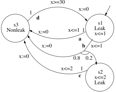
Fig. 1: A probabilistic timed automaton for a simple gas burner.
timed automaton does, except that it has to select a probability distribution at each discrete step.
We denote byZC(G) the set of all clock zones occurring inG,
ZC(G)= {inv(s)∈ZC| s∈ S}∪ {τs(p)∈ZC|s∈ Sand
p∈ prob(s)}.
Example 1. Fig. 1 shows a probabilistic timed automaton for a simple gas burner.
The system starts at the node s1, with the
gas valve is opened without flame being on,
hence gas is leaking. At this state, there are
two nondeterministic choices. The first choice denoted by transitionais that with the probability
1, the flame is turned on within one second (x ≤
1) and the system moves to node s3 for which
gas is not leaking. The second choice denoted by transitionbis as follows: with the probability 0.8, the flame is turned on within one second and
the system moves to nodes3 for which gas is not
leaking, and with probability 0.2 the flame fails to be on within one second, and the system moves to
node s2 for which gas is still leaking. In state
s2, with probability 1, the gas valve is closed
successfully within 2 seconds since the time the system entereds1 last time, and the system moves to node s3. At state s3, the gas burner will move to the state s! only after it has stayed there at least 30 seconds. Formally, in this example, the
function probis given as: prob(s1) = {p0,p1},
prob(s2) = {p2}, prob(s3) = {p3}, where
p0(s3,{x}) = 1, p1(s3,{x}) = 0.8, p1(s2,∅) = 0.2. p2(s3,{x}) = 1, p3(s1,{x}) = 1, and
τs1(p0) = τs1(p1) = {x ≤ 1}, τs2(p2) = {x ≤ 2}
and τs3(p3) = {x ≥ 30}. The function inv is
defined as inv(s1) = {x ≤ 1},inv(s2) = {x ≤ 2} andinv(s3)=true. The labels of states are given by functionLdefined asL(s1) = L(s2) = leak, andL(s3)=nonleak.
As in [12] we use probabilistic timed structures as underlying semantics model for PTA.
Definition 2. A probabilistic timed structure M
is a labeled Markov decision process(Q,Steps,L)
whereQis a set of states, Steps:Q → 2R≥0×µ(Q)
is a function which assigns to each state q ∈ Q
a set Steps(q) of pairs of the form (t,p), where t∈R≥0and p∈µ(Q), and L:Q →2APis a state labeling function.
Function Steps specifies the set of transitions
that Mcan choose nondeterministically at each
state. Therefore, if at state q ∈ Q, M chooses
(t,p) ∈ Steps(q), then after t time units have elapsed, a probabilistic transition is made to state
q0 with probability p(q0). A path of M is a
nonempty finite or infinite sequence:
ω = q0
t0,p0
−→q1
t1,p1
−→q2
t2,p2
−→. . .
whereqi∈ Q, (ti,pi)∈Steps(si), and pi(qi+1)>0 for all 0≤i≤ |ω|. For a given probabilistic timed structuresMwe denote byPathf in (Pathin f) the set of finite (infinite) paths, and by Pathf in(q) (Pathin f(q)) the set of paths in Pathf in (Pathin f)
that start from state q. Let ω be infinite. A
position of ω is a pair (i,t), where i ∈ N and
t ∈ R≥0 such that 0 ≤ t ≤ ti. The state at
position (i,t) is denoted by stateω(i,t). Given two positions (i,t) and (j,t0) of ω, we say (j,t0) precedes (i,t) (in ω, written by (j,t0) ≺ (i,t)) if
j<ior j=iandt0<t.
Definition 3. For any path ω of a probabilistic timed structure M and 0 ≤ i ≤ |ω| we define
Dω(i), the elapsed time until the ith transition, as follows:Dω(0)=0and for any1≤i≤ |ω|:
Dω(i) = Pi−1
An infinite path ω is said to be divergent iff
for any t ∈ R≥0, there exists j ∈ N such that
Dω(j) > t. Let ω be infinite. For each state
q ∈ Q, we define a {0,1}-valued function
qω :R≥0→ {0,1}as
qω(t)=
1 iffthere exists a position (i,t0) s.t.
t0 >0,stateω(i,t0)=qand
t=Dω(i)+t0,
0 otherwise.
Intuitively, qω(t) = 1 means that in the path ω, stateqis present in an interval (t−δ,t] for some
δ >0, and otherwiseqω(t)=0.
The concept of strategy was introduced in the literature (see, e.g. Kwiakowska [12]) as a schedule for resolving all the nondeterministic
choices of the model. Note that we have
restricted ourselves to discrete probability
distributions only.
Definition 4. A strategy (or scheduler) of a probabilistic timed structure M = (Q,Steps,L)
is a function A mapping every nonempty finite path ω of M to a pair (t,p) such that A(ω) ∈
Steps(last(ω)), and the empty path to a state in
Q. LetAbe the set of all strategies ofM.
Let us denote a prefix of lengthiofωbyω(i), and define for a given strategyA
PathAf in=
ω∈Pathf in
A()=ω(0), and
step(ω,i)=A(ω(i)) for 0≤i<|ω|
PathAin f =
ω∈Pathin f
A()=ω(0), and
step(ω,i)=A(ω(i)) for 0≤i
Recall that step(ω,i) returns the label of the
ith transition in ω. From Definition 4, all ω
in PathAf in and PathAin f start from the same state defined byA(), and intuitively they represent the
behaviors ofMaccording to the schedulerA,
A sequential Markov chain MCA =
(PathAf in,PA) is associated with a strategy A
in a natural way to express the executions of M
according toA, wherePAis defined as
PA(ω, ω0) =
p(q) ifA(ω)=(t,p) and
ω0=ω−→t,p q,
0 otherwise.
LetFPathA be the smallestσ-algebra onPathAin f
which for all ω0 ∈ PathAf in contains the sets
{ω | ω ∈ Pathin fA andω0is a prefix ofω}.
Let ProbAf in : PathAf in → [0,1] be the
mapping defined inductively on the length of paths in PathAf in as follows. If |ω| = 0 then
ProbAf in(ω)=1. Letω0 ∈PathAf inbe a finite path ofA. Ifω0 =ω−→t,p qfor someω∈PathAf in, then we let ProbAf in(ω0) = ProbAf in(ω)PA(ω, ω0).
The measure ProbA on FPathA is the
unique measure such that ProbA({ω | ω ∈
PathAin f andω0is a prefix ofω}) = ProbAf in(ω0). In this paper, we assume that the strategies under consideration are divergent in the probabilistic
sense, i.e. we assume that for any strategy A,
ProbA({ω|ω∈PathAin f andωis divergent})=1. We now define the behavior of probabilistic timed automata by associating every probabilistic timed automaton with a probabilistic timed structure. A state of the structure consists of a state of the automaton, and a valuation for the clock variables.
Definition 5. For any probabilistic timed automaton G as in Definition 1, define the probabilistic timed structure MG = (QG,StepsG,LG)as follows.
• QG ={hs, νi | s∈ S, ν∈(R≥0)C}
• The function StepsG : QG → 2R ≥0×µ(Q
G) assigns to each state in QG a set of
transitions, each of which takes the form
(t,p¯) where t ∈ R≥0 and p is a discrete¯ probabilistic distribution on Q, and is defined as:
– (t,p¯) ∈ StepsG(hs, νi) if there exists p∈ prob(s)such that (a) the valuation
ν+t satisfies τs(p) andν+t0 satisfies
inv(s) for all 0 ≤ t0 ≤ t, and (b) for any hs0, ν0i ∈ QG: p¯(hs0, ν0i) =
P
X⊆C∧(ν+t)[X:=0]=ν0 p(s0,X). For
convenience, we refer to p as having¯
type p, denoted bytype( ¯p)= p. – Let (t,p¯) ∈ StepsG(hs, νi) if (a) the
valuation ν+t0 satisfies inv(s) for all
QG: p¯(hs0, ν0i) = 1 if hs0, ν0i = hs, ν+ti, and p¯(hs0, ν0i =0otherwise. We refer to p as having type¯ >, i.e. type( ¯p)=>.
• The labeling function L:Q →2APis defined as: LG(hs, νi)=L(s)for allhs, νi ∈ QG.
The second item of the definition of the
functionStepsallows the automaton to stay in a
state forever from a time if the invariant for the state is never violated from that time, and the corresponding path is infinite.
Any strategy for the timed structure MG
is also called strategy for probabilistic timed
automatonG.
Example 2. The following path is a path of (a strategy of) the timed structure of the timed automaton in Fig. 1:
ω = hs1,0i−→ h.9,.8 s3,0i−→ h31,1 s1,0i−→.7,.2 hs2, .7i1−→ h.2,1 s3,0i−→ h30,1 s3,30i100−→,1 hs3,130i100−→,1. . . .
For a given infinite divergent path
ω of MG, for an atomic proposition
P ∈ AP, let us define a {0,1}-valued
function Pω : R≥0 → {0,1} by Pω(t) =
max{qω(t) | q=hs, νi ∈ QGandP∈ L(s)} (note that there can be several regions hs, νi in the
path ω for which P ∈ L(s)). So, Pω(t) = 1
means that there is an semi-interval (t− δ,t] in
which Pholds. Otherwise,Pω(t) = 0. Since we
have assumed that ω is divergent, Pω has the
finite variability, i.e. it has only finite number of discontinuity points within any finite interval.
3. Probabilistic Duration Calculus
In this section we introduce a simple form of Probabilistic Duration Calculus. A complete probabilistic interval logic (which DC is based on) with a proof system has been introduced in [5]. However the definition of the semantics in that paper for the calculus is rather complicated
and less intuitive. The calculus introduced
in this paper has an intuitive semantics based
on probabilistic timed automata, and has a simple grammar that allows to write formulas to reason about the probability of the satisfaction of a duration formula by a probabilistic timed automaton as well as to specify real-time properties of the system itself.
Definition 6. Let R stand for relations (e.g. ≤
,=), and F stand for functions (e.g. +, −). The syntax of Probabilistic Duration Calculus is defined as follows.
Φ ::= Ψ|[Ψ]wλ| ¬Φ|Φ∧Φ,
Ψ ::= R(η, . . . , η)| ¬Ψ|Ψ∧Ψ|Ψ;Ψ,
η ::= R S |F(η, . . . , η),
S ::= 1|P|¬S |S ∧S,
where Φ stands for Probabilistic Duration Calculus formulas, Ψ stands for Duration Calculus formulas, η stands for duration terms, S stands for state expressions, and P is a symbol in the set of atomic proposition AP.
We will use a probabilistic timed automaton
G as underlying model to define the semantics
for Probabilistic Duration Calculus formulas as
well as for Duration Calculus formulas. LetIntv
denote the set of all intervals onR≥0.
Given a path ω of MG according to a
strategyA. The interpretation of state expression
S is a {0,1}-valued function ISω : R≥0 →
{0,1} defined inductively as: Iω
1(t) = 1
for all t ∈ R≥0, IPω = Pω where Pω is
defined as in Section 2, I¬ωS = 1 − IωS, and
ISω1∧S2 = min{ISω1,ISω2}. (Note that the operations
on functions is defined point-wise.) The
interpretation of a termηis a functionIηω:Intv→
R≥0 defined as IRω
S([a,b]) =
Rb
a I
ω
S(t)dt, and
Iωf(η1,...,ηk)([a,b]) = f(Iηω1([a,b]), . . . ,Iηωk([a,b])) for any interval [a,b]∈Intv.
A model for DC formulas is a pair (ω,[a,b])
of a divergent path ω and an interval [a,b].
The semantics of Duration Calculus formulas is essentially the satisfaction relation |= between a
model (ω,[a,b]) and a DC formula Ψ which is
defined as follows.
• (ω,[a,b])|=R(η1, . . . , ηk) iff
• (ω,[a,b])|=¬Ψiff(ω,[a,b])6|= Ψ,
• (ω,[a,b])|= Ψ1∧Ψ2 iff(ω,[a,b])|= Ψ1 and (ω,[a,b])|= Ψ2,
• (ω,[a,b])|= Ψ1;Ψ2 iff(ω,[a,m])|= Ψ1 and (ω,[m,b])|= Ψ2 for somem∈[a,b].
The probability measure ProbA will come to
play role in the definition of semantics of PDC formulas. A model for a PDC formula consists
of a strategy AofMG and a time pointt(recall
thatA defines an “initial” state, not necessary to be hs¯,0i; to be meaningful, we may need the restriction that the “initial” state of A is hs¯,0i, we will assume this whenever necessary). The
satisfaction relation |=PDC between PDC models
(A,t) and PDC formulasΦis defined as:
• For a DC formulaΨ, (A,t)|=PDC Ψiff
ProbA({ω| ω ∈ PathAin f and ωis divergent and
(ω,[0,t])|= Ψ})=1,
• For a DC formulaΨ, (A,t)|=PDC [Ψ]wλ iff
ProbA({ω| ω ∈ PathAin f and ωis divergent and
(ω,[0,t])|= Ψ})≥λ,
• (A,t)|=PDC ¬Φiff(A,t)6|=PDC Φ
• (A,t)|=PDC Φ1∧Φ2 iff(A,t) |=PDC Φ1 and (A,t)|=PDC Φ2.
The reason for a using a strategy to define a model of PDC formulas is clear since the probability is defined just for subsets of paths induced byA, not for a single path. But the reason for selecting an interval of the form [0,t] instead of [a,b] is just for convenience. The computation
of ProbA(B) for a set B of paths satisfying a
DC formula Ψ in an interval [a,b] needs the
prefixes in the whole interval [0,b] of paths in
B. Intuitively, a strategyAof probabilistic timed
automaton G satisfies a DC formula Ψ in the
probabilistic setting at a timetiffthe set of infinite
divergent pathsωproduced byAthat satisfyΨin
the interval [0,t] has the probability 1.
A DC formula Φ is said to be valid iff
(ω,[a,b]) |= Φholds for any probabilistic timed
automaton G, any path ω of G, and any time
interval [a,b]. A PDC formula Φ is said to be
valid iff(A,t)|=PDCΦholds for any probabilistic timed automatonG, strategyAofG, andt∈R≥0. In [17, 2] a proof system for DC for deriving
valid formulas has been presented. It follows
directly from the definition of semantics that PDC is a conservative extension of DC. Besides, some obvious properties of the probabilities can be translated into valid formulas in PDC easily.
These observations are formulated in the following theorem.
Theorem 1. For any DC formulasΦ,Φ1andΦ2
• [Φ]w1⇔Φis a valid PDC formula,
• IfΦis a valid DC formula, then it is a valid PDC formula,
• ((Φ1⇒Φ2)∧[Φ1]wλ) ⇒[Φ2]wλ is a valid PDC formula
• ¬(Φ1∧Φ2)∧[Φ1]wλ1∧[Φ2]wλ2 ⇒[Φ1∨
Φ2]wλ1+λ2is a valid PDC formula.
Proof. Straightforward from the definition of
semantics of DC and PDC. 2
As usual in DC, we use the following
abbreviations: `b=
R
1, T rueb=` ≥ 0,
3Ψb=T rue;Ψ;T rue (there exists a subinterval
for which Ψ is satisfied), 2Ψb=¬3¬Ψ (for all
subintervalsΨis satisfied),dSeb=R S =`∧` >0. Note that PDC can express the safety and bounded liveness properties, but not unbounded liveness properties. For example, PDC formula
2(dPe;` >b⇒` ≤ b;dQe) says that it is almost
certain that whenever P becomes true for
non-zero time period, Q must become true for
non-zero time period withinbtime units.
Example 3. Let us consider the simple gas burner in Example 1 (see Fig. 1). Let one of the requirements for the gas burner is that for any observation interval the length of which is not shorter than 60 seconds, the accumulated leakage time is not longer than 4% of the length of the observation interval. This requirement is
formalized as a DC formula R b= 2(` ≥ 60 ⇒
R
(s3,60)
(s3,60) (s3,30) (s3,30) 30
1
30
1
(s3,60)
(s3,60) (s3,30) (s3,30) 30
1
30
1 (s2,1)
(s2,2) 1
1 (s1,1)
(s3,0) 0.8 0.2
(s3,0)
(s3,30)
(s1,0) 1 1 30
(s3,60)
(s3,60) (s3,30) (s3,30) 30
1
30
1
(s3,60)
(s3,60) (s3,30) (s3,30) 30
1
30
1 (s2,1)
(s2,2) 1
1 (s1,1)
(s3,0) 0.8 0.2
(s2,1)
(s2,2) 1
(s3,0)
(s3,0)
(s3,30)
(s1,0) 1 1 30 1 1
(s1,1) (s1,0)
0.2 0.8
(s3,0)
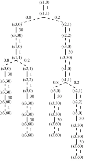
Fig. 2: A part of a strategyAfor the simple gas burner.
definition”). Let ω be given as in Example 2.
Then, (ω,[0,60])6|=(`≥60⇒R leak≤4%∗`). This is so because the accumulated time for the leakage in the interval [0,60] is.9+.7+1.2=2.8 which is longer than 4%∗60 (=2.4).
Let strategy A that schedules the system
producing the paths be as shown by the tree in Fig. 2 in which the dashed edges represent discrete transitions labeled with probability, and the non-dashed edges represent time advance transitions labeled with their corresponding amount of time units. Only those paths that have a prefix represented by the leftmost branch of the tree, satisfy the requirementRin the interval [0,60]. The set of these paths has the probability 0.8∗0.8 = 0.64. Hence, (A,60) |= [R]w.6 (note
that this example is for the sake of illustrating the concepts only).
4. Model checking probabilistic timed automata against PDC properties
Duration Calculus formulas are highly
undecidable, only a very small class of chop free
formulas is decidable (see [18]). In this section, we develop a technique to verify if a set of all PDC models generated by a probabilistic timed
automatonGsatisfies a PDC formula in discrete
time. Namely, we consider the problem to decide
A,t |=PDC [Ψ]wλ for all A ∈ Aand all t ∈ R≥0,
where A is the set af all integral strategies of a
timed automatonG. In the sequel, for simplicity
by saying “strategy” we actually mean “integral strategy” unless differently stated.
Depending on different forms of model sets we can have different model checking problems as:
1. Single strategy single time: given a strategy
A, given a timet, to decideA,t|=PDC [Ψ]wλ. This problem is decidable. It is so because the fact that a path ωsatisfies Ψin [0,t] or not depends only on the smallest prefixω(i) such that Dω(i) ≥ t. The set {ω0 | ω0 ∈
PathAf inandDω0(|ω0|) ≥ tandDω0(|ω0| −
1) < t} is finite, and computable if A
is computable. From the assumption, the
set {ω0 | ω0 ∈ PathA
f inandDω0(|ω 0|) ≥
tandDω0(|ω0|−1)<tand (ω0,[0,t])|= Ψ}is computable, and finite. Hence, ProbA({ω ∈
PathAf in|(ω,[0,t])|= Ψ}) is computable, and therefore,A,t|=PDC[Ψ]wλis decidable.
2. Multiple strategy single time: Given a
set of strategies A which have a finite
representation, given a time t, decide
A,t |=PDC [Ψ]wλ for all A ∈ A. If A is finite, the problem is decidable. Hence the decidability of the problem depends on the form of the computable setAof strategies. 3. Single strategy with arbitrary time: Given a
strategyAwhich has a finite representation,
decide if A,t |=PDC [Ψ]wλ for all t ∈
R≥0. This problem in general is undecidable
even for λ = 1 because DC is undecidable
in general.
4. Multiple strategy with arbitrary time: Given
a set of strategies A which have a finite
representation, decide A,t |=PDC [Ψ]wλ for all A ∈ Aand allt ∈R≥0. This problem is most general, and undecidable because DC is undecidable in general.
In this section, we will restrict ourselves to some instances of the problems mentioned in the items 3 and 4.
We are interested specially in the PDC formulas of the form [Ψ]wλ, whereΨhas the form
2(a ≤ ` ≤ b ⇒ Pk i=1ci
R
Pi ≤ M) called linear
duration invariants (LDI) [7], where M, a and
b are integers, b could be ∞. A dependability
requirement for the simple gas burner could be
expressed as [2(` ≥ 60 ⇒ R leak ≤ 4% ∗
`)]w.99 which says that with the probability .99,
the accumulated time for gas leaking is not more than 4% of the observation time whenever the observation time is longer than 60 seconds. So, the (A,[0,105]) |= [2(` ≥ 60 ⇒ R leak ≤
4% ∗ `)]w.99 for any strategy A says about the
reliability of the gas burner: its requirement is satisfied with the probability .99 whenever it is operated for less than 105seconds.
For simplicity and as motivated by the discretisability of LDI [9] (i.e. an LDI is satisfied by all models if and only if it is satisfied by all integral models), we restrict ourselves to those strategies in which each transition is of the form (t,p) wheret∈Nonly.
Now, we recall a very important technique from timed automata with some adaptations to probabilistic timed automata. Let, in the sequel,
Gbe a PTA.
Integral Region Graph. The key idea for reducing the state space of timed automata to a finite space is the clock equivalence relation introduced in [16]. In this subsection we recall this standard notions restricted to the set NC of
integral clock valuations. Let c be the max of
integers occurring in clock constraints inG.
Definition 7. The valuationsν, ν0∈NCare clock equivalent, denoted byνν0iff
1. ∀x ∈ C, eitherν(x)=ν0(x), or bothν(x)>c andν0(x)>c,
2. ∀x,x0∈ C, eitherν(x)−ν(x0)=ν0(x)−ν0(x0), or bothν(x)−ν(x0)>c andν0(x)−ν0(x0)>c
One important property of the clock
equivalence relation is that it has finite
index and the valuations from the same
equivalence class satisfy the same set of clock constraints as formulated as the following lemma (taken from [16, 9]):
Lemma 1. Letν, ν0 ∈ NC, X ∈ 2C, and ν ν0.
Then
1. ν[X:=0]ν0[X:=0]
2. for any zone ζ ∈ ZC(G) appearing in the
description of G, νsatisfiesζ if and only if
ν0satisfiesζ.
LetG be the set of all equivalence classes of
. An equivalence classα ∈ Gsatisfies a clock
constraint ζ ∈ ZC(G) iff ν satisfies ζ for some
ν ∈ α. From the item 2 of Lemma 1, it follows
thatαsatisfies a clock constraintζif and only ifν satisfiesζfor anyν∈α. An equivalence classβis said to be the successor of an equivalence classα, denoted bysucc(α) ifffor eachν∈α, there exists
t ∈ N such that ν+t ∈ β and ν+ t0 ∈ α∪β
for all t0 ≤ t and t0 ∈ N. Let dα = sup{t ∈
N | ν ∈ αandν + t ∈ succ(α) andν + t0 ∈
α∪βfor allt0 ≤tandt0∈N}. It follows from the definition ofsucc(α) that eitherdα =1 ordα =∞.
The latter happens only when succ(α) satisfies
x>cfor allx∈ C. The nondeterministic discrete
time behaviors of PTA G can now be described
by the region graphR(G) defined as follows.
Definition 8. The region graph R(G) is the Markov decision process(V∗,Steps∗,L∗), where
• the vertex set V∗b={hs, αi | s∈ Sandα∈ G
andαsatisfies inv(s)}, and
• the transition function Steps∗ : V∗ → 2N×µ(V∗) is defined as follows. For each vertexhs, αi ∈V∗:
1. If the invariant condition inv(s)
is satisfied by succ(α) then for any hs0, βi ∈ V∗, let psuccs,α (hs0, βi)
=
(
1 ifhs0, βi=hs,succ(α)i,
0 otherwise.
Then (t,pssucc,α ) ∈ Steps∗(s, α) for any
2. If there exists p0 ∈ prob(s) such that αsatisfies the enabling condition
τs(p0), then for any hs0, βi ∈ V∗ let
psp,α0 (hs0, βi) =
P
X⊆C,α[X:=0]=βp0(s0,X). Then,(0,psp,α0 ) ∈Steps∗(hs, αi). In this
case, we saytype(psp,α0 )= p0.
In the definition of Steps∗ the item (1)
represents the time transitions, and the item (2) represents the discrete transitions.
Definition 9. A strategy A∗on the region graph is a function mapping every nonempty finite pathω∗ of R(G)to a pair of integral time t and distribution p such that (t,p) ∈ Steps∗(last(ω∗)), and mappingtohs¯,0i.
By the definition of transition functionSteps∗,
the number of the (time) transitions of R(G)
between a node (s, α) and (s,succ(α)) is infinite
when dα = ∞. In the graph, those transitions
are combined into one transition which is labeled by (∗,1), where 1 is the probability distribution assigning probability 1 to the transition from (s, α) to (s,succ(α)). This transition expresses that we can choose nondeterministically an arbitrary integer for time step, and then with the probability 1, move to the region (s,succ(α)).
Therefore, a strategy A of R(G) will replace ∗
by an integer each time it travels through this transition. From the definition of the region graph
R(G) and the timed structure MG, the paths in
R(G) and the paths in MG are closely related.
Namely, if inMG there is a transitionhs, νi t,p¯
−→ hs0, ν0i, where type( ¯p) = p0 and t ∈ N then
in R(G) there is a path hs, α0i −→t1,p1 . . . t−→k,pk
hs, αki
0,ps,αk p0
−→ hs0, βi such that type(pi) = >,
αi = succ(αi−1) for 1 ≤ i ≤ k,type(p
s,αk
p0 ) = p0,
ν ∈ α0, ν0 ∈ β, inv(s) is satisfied by all αi, t =
t1+. . .+tk, andαksatisfiesτs(p0). Furthermore, if in MG there is a transition hs, νi
t,p¯
−→ hs, ν0i where type( ¯p) = > and t ∈ N then in R(G)
there is a path hs, α0i t−→1,p1 . . . −→ htk,pk s, αki such thattype(pi) =>, for 1≤ i≤k,αi = succ(αi−1)
and satisfiesinv(s),ν∈α0,ν0∈αk,t=t1+. . .+tk.
Conversely, for each transition inR(G) of the form hs, αi t,p
s,α
−→ hs0, βi, for any ν ∈ α there is a transition hs, νi −→ ht,p¯ s0, ν0i in MG with type( ¯p)=type(ps,α) andν0∈β.
From this observation each strategyA∗ofR(G) corresponds one-to-one with an integral strategy
A of MG in a sense that will be made precise
soon.
With each strategyA∗ofR(G) we can associate a Markov chain MCA∗ = (PathAf in∗,PA∗) where forω∗, ω0∗ ∈PathAf in∗ andhs, αi,hs0, α0isuch that
last(ω∗)=hs, αi,
PA∗(ω∗, ω0∗)=
ps,α ifA∗(ω∗)=(t,ps,α) and
ω0∗=ω∗(t,ps
,α)
−→ hs0, α0i,
0 otherwise.
Then, the probabilistic measure ProbA∗
on the smallest σ-algebra FA∗
Path on
PathAin f∗ containing the sets of the forms
{ω∗ | ω∗ ∈ Pathin fA∗ andω0∗is a prefix ofω∗} for any ω0∗ ∈ PathAf in∗ is defined as before for
a probabilistic timed structure. Recall that
from probabilistic timed automaton G, we have
defined a probabilistic timed structureMGwhich
generates the probabilistic measure ProbA on
the smallest σ-algebra FA
Path on Path
A
in f. From the relationship between strategies A∗ of R(G)
and strategies AofMG observed earlier we can
derive a relationship forProbA∗ andProbAwhich plays key role in model checking PDC formulas.
The relation betweenR(G) andMG is expressed
formally as:
Lemma 2. Let A be an integral strategy of probabilistic timed automaton G (i.e. an integral strategy ofMG). Then, there exists an strategy A∗
of the integral region graph R(G)and an one-to-one mappingsγ:PathAin f →PathAin f∗ such that:
1. ProbA(Ω)=ProbA∗(γ(Ω))for allΩ∈ FPathA ,
2. Pω(t) = Pγ(ω)(t) almost everywhere inR≥0 for allω∈Pathin fA
Proof. Letγbe the homomorphism defined from the relation between transitions inMG andR(G) observed as above. Given strategyA, strategyA∗
A by splitting one step (t,p) into several time steps (1,1), . . . ,(1,1),(0,p) as given by mapping
γ. Item 2 follows directly from the construction
ofA∗, and Item 1 follows from the fact that for all
ω ∈ PathAf in, ProbAf in(ω) = ProbAf in∗ (γ(ω)). The
detailed proof is omitted here. 2
Item 2 of Lemma 2 implies that (ω,[a,b])|= Ψ if and only if (γ(ω),[a,b]) |= Ψ for any DC
formula Ψ, for any ω ∈ PathAin f and interval
[a,b]. Combined with Item 1, this implies that
A,t|=PDC Φif and only if A∗,t |=PDC Φfor any PDC formulaΦandt∈R≥0.
Depending on how integral strategyA ofG is
given, the corresponding strategy A∗ofR(G) can be found easily based onA. For simplicity, firstly we consider the problem to decide ifA,t|=PDC Φ fort∈R≥0. Now consider the following case for
PDC formulaΦ:
Φ =[Ψ]wλ, Ψ =2Ψ1 (1)
where Ψ1 is a DC formula (to be more general
Ψ is not necessary to be LDI). We have that
(
ω
ω∈PathAin f∗ andωis divergent and (ω,[0,n])|= Ψfor alln∈N
)
= T
n≥0 (
ω
ω∈PathAin f∗ andωis
divergent and (ω,[0,n])|= Ψ
)
.
Because the set sequence
{ω | ω ∈ PathAin f∗ and ω is divergent and
(ω,[0,n]) |= Ψ} is decreasingly monotonic
(according to the set inclusion relation) when n
increases, we have that ProbA∗({ω |ω ∈ PathAin f∗
and ω is divergent and (ω,[0,n]) |= Ψ for all
n ∈ N}) = infn∈N{Prob A∗
({ω | ω ∈ PathAin f∗ and
ωis divergent and (ω,[0,n])|= Ψ}).
Hence, if we can compute ProbA∗({ω | ω ∈
PathAin f∗ andωis divergent and (ω,[0,n])|= Ψfor alln∈N}), we can solve the problem to decide if
A∗,t|= Φfor allt≥0.
LetPbe a path in the region graphR(G) that
generates a DC model not satisfyingΨ1. Assume
that a path in Pathin fA∗ that does not satisfy DC
formula Ψ in an interval if and only if it has
a prefix that includes P. Then all the paths in
PathAin f∗ that satisfy Ψ for any interval are those that do not includeP. From integral graphR(G),
we can find all such paths Pthat can generate a
DC model not satisfyingΨ1, and can construct a
graph that generate all the paths in PathAin f∗ that
do not include any such pathP(i.e. those paths
that satisfy Ψfor any interval). We assume that
any two paths in P are not nested (if for two
paths in P, one is nested in the other, we can
remove the later without changing the meaning of P). From the labels of the constructed graph, the probability of the set of paths can be calculated. To apply this procedure we need: (a) a technique to construct the finite set of paths PinR(G) that correspond to all DC models that do not satisfy
Ψ1, (b) the set of paths in Pathin fA∗ that do not include any such pathPare finitely representable by a graph, and (c) a technique to compute the probability of the set of infinite paths resulting from item (b).
Regarding Item (a), the following lemma is from [9, 10], which says that given a linear duration invariantΨ, the set of paths that do not satisfyΨis computable by searching inR(G).
Lemma 3.
1. Given a pathω∈PathAin f∗ . A linear duration invariant Ψ is satisfied by model (ω,[a,b])
for any interval [a,b] if and only if it is satisfied by model(ω,[m,n])for any integral interval[m,n].
2. The set of paths of integral region graph R(G)that correspond to a DC integral model that does not satisfyΨis constructable.
Regarding Item (b), we have to restrict
ourselves to the class of so-called finitely
representable strategies A∗ of the region graph
R(G). A strategy A∗ of R(G) is finitely
representable ifffor any pathω∗ofR(G) the value ofA∗(ω∗) depends only on the suffix of the length
k of ω∗ for a fixed k. An finitely representable strategy A∗ ofR(G) for the case k = 1 is called
simple strategy. Such a finitely representable
strategy will be represented by a graph with no nondeterminism, complete probabilistic choices, and fully embedded inR(G).
(VA∗,Steps
A∗,LA∗) which is embedded in the
region graph R(G) = (V∗,Steps∗,L∗) by a mapping ρ, where ρ : VA∗ → V∗, and the
following conditions are satisfied:
• There is an initial node called v0, and
ρ(v0)=hs¯,0i,.
• G(A∗) is deterministic, i.e. StepsA∗(v) has
only one element, denoted by StepsA∗(v)
itself,
• LA∗(v)=L∗(ρ(v))for all v∈VA∗
• Let StepsA∗(v) = (t,p), where p is a
distribution in µ(VA∗). The restriction ofρ
on {v0 ∈ VA∗ | p(v0) > 0} is an one-to-one
mapping, and the distributionρp defined by ∀s ∈V∗•ρp(s)= max{p(v0)|ρ(v0) = s}(by
our convention,max∅ =0) is a distribution inµ(V∗), and(t, ρp)∈Steps∗(ρ(v)).
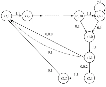
Figure 3 shows the integral region graph of Simple Gas Burner in Fig 1 and graph
representations for finitely representable
strategiesA∗1andA∗2. The embedding mappingρ maps a node in A∗1 and A∗2 to the node with the same label in the integral region graph.
Regarding Item (c) of the condition for applying the checking procedure, we have
Lemma 4. Given a graph representation of a finitely representable strategy A∗, G(A∗) = (VA∗,Steps
A∗,LA∗). Given a finite set Pof finite
paths of G(A∗). Let Ω be the set of all infinite paths of G(A∗) starting from v0 which do not include any path inP. The probability ProbA∗(Ω)
is computable.
Proof. Let ∆(v) be the set of all infinite paths
of G(A∗) starting from v which do not include
any path in P, A∗v be the strategy represented
by G(A∗) with v as initial node, and P(v) =
ProbA∗v(∆(v)). Let for each v, P(v) = {ω00|ω00 ∈
Pandω00starts fromv}. Letv+be the set of
one-step paths formed by outgoing edges ofv. Then,
∆(v) satisfies:∆(v)=
(∪e∈v+(e∆(last(e))))\(∪eω∈P(v)eω∆(last(ω))).
Although all paths inPare not nested in one
another, but some of them may overlap some suffixes of ω for a given finite path ω. Let Pω be the set of those such paths ofP,Pω = {ω0 ∈ P|ω0= xzandω=yxfor some pathsx,,y,z}.
Then
ω∆(last(ω))\∆(last(e))= ∪ω0∈P
ω(ω ω0)ω0∆(last(ω0)),
where for ω = yx (x , ) and ω0 = xz ∈ Pω
we define ω ω0 = y. From the definition
of the functions ProbA∗v, v ∈ VA∗ it follows
ProbA∗last(e)(∆(last(e))\ω∆(last(ω)))=
ProbA∗last(e)(∆(last(e)))−
ProbA
∗
last(e)(ω∆(last(ω)))+
ProbA∗last(e)(∪ω0∈P
ω(ω ω0)ω0∆(last(ω0)))
Because all paths in P are not nested in one
another, for eω,eω00 ∈ P(v) with ω , ω00, we
have ω∆(last(ω)) ∩ ω00∆(last(ω00)) = ∅. For simplicity, we assume that for ω01, ω02 ∈ Pω with ω01 , ω02, (e(ω ω10)ω01∆(last(ω01))) ∩
(e(ω ω02)ω02∆(last(ω02))) = ∅. (without this assumption, we have to modify the technique a little). Therefore, the definition of ProbA∗n, n∈VA∗ implies
ProbA∗v(∆(v))= P
e∈v+ProbA ∗
f in(e)Prob A∗
last(e)(∆(last(e)))− P
eω∈P(v)ProbA
∗
f in(eω)Prob A∗
last(ω)(∆(last(ω))))+ P
eω∈P(v)Pω0∈P
ω(Prob
A∗
f in(e(ω ω 0)ω0)×
ProbA
∗
last(ω0)
(∆(last(ω0)))) Let us denote
ProbA∗v(∆(v)) by P(v). This means that P(v), v∈VA∗ satisfy:
P(v)=
P
e∈v+ProbA ∗
f in(e)∗P(last(e))−
P
ω∈P(v)ProbA
∗
f in(ω)∗P(last(ω))+
P
eω∈P(v)Pω0∈P
ωProb
A∗ f in(e(ω
ω0)ω0)P(last(ω0)) and P(v) = 1 if no path inPis reachable fromv. These conditions form a linear equation system forP(v),v∈VA∗. Solving it, we can find the value of P(v0) which is the
value ofProbA∗(Ω). 2
The following theorem follows immediately from these lemmas.
integral strategy A of probabilistic timed automaton G satisfiesΦat any time point t.
Decision Procedure 1. Given a PTA G, given
a finitely representable strategy A of MG, our
procedure to decide ifA,t|=PDCΦfor allt∈R≥0,
whereΦ = [Ψ]wλ, Ψ = 2Ψ1 andΨ1 is an LDI,
consists of the following steps:
1. Construct the integral region graphR(G) for
G.
2. Construct the finitely representable strategy
A∗ofR(G) corresponding toAaccording to Lemma 2.
3. Construct the set P of all paths R(G) that corresponds to a a DC model that does not satisfyΨ1 (using the technique mentioned in Lemma 3.
4. Find a graph representation of A∗ as
mentioned in Definition 10.
5. Let Ω be the set of all infinite paths
of G(A∗) starting from v0 which do not
include any path in P. Compute the
probabilityProbA∗(Ω) using the technique in Lemma 4.If this probability is greater thanλ, then the answer is positive. Otherwise, give the negative answer.
Note that using the same techniques, the model checking problem mentioned in Item 3 at the beginning of this section is solvable for a PDC
formulaΦof the form (1) where Ψis a formula
expressing the bounded liveness2(dPe;` > b ⇒
` ≤ b;dQe). In general, the problem is solvable for the case that the set of paths of integral region
graph R(G) that correspond to a DC integral
model that does not satisfyΨis constructable. In [10] we proposed some form for such formulas.
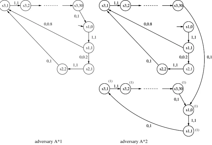
Example 4. Fig. 3 shows the integral region
graph R(G) of the simple gas burner in Fig. 1,
and Fig. 4 shows two strategies A∗1andA∗2of the region graph. We will decide which one among
A∗1andA∗2satisfies the requirementRin Example 2 with a probability not lower than 0.6 using the technique mentioned above.
Any infinite path ω of strategy A∗1 that goes through the path
P1 = (s1,0)(s1,1)(s2,1)(s2,2) contains a model
1,1 1,1
0,1 0,1
1,1 0,0.8
0,1
s3,1 s3,2 s3,30 s3,>30
s1,0
s1,1
0,0.2
s2,1 s2,2
0,1
1,1
*,1
Fig. 3: Integral Region Graph for Gas Burner.
that does not satisfy R. Indeed, ω containing
P1 should contain an interval with length 60 for
which the accumulated leakage time is at least
3 (3 > 2.4 = 4% ∗ 60). Any infinite path
ω of strategy A∗1 that does not contain P1 as a
sub path satisfies R in any interval. Using the
technique in the proof of Lemma 4, we have the following system of linear equationsP(hs1,0i)=
P(hs1,1i −1∗0.2∗1∗P(hs2,2i
P(hs1,1i)=0.8P(hs3,1i)+0.2P(hs2,1i)
P(hs2,1i)= P(hs2,2i)=P(hs3,1i)=. . .
= P(hs1,0i) Solving this system, we get
P(hs1,0i) = 0. Hence, we can conclude that A∗1
does not satisfies requirement [R]w0.6.
Now consider strategyA∗2. The linear equation system for this case is: P(hs1,0i) = P(hs1,1i − 1∗0.2∗1∗P(hs2,2i
P(hs1,1i)=0.8P(hs3,1i)+0.2P(hs2,1i)
P(hs2,1i)= P(hs2,2i)=P(hs3,1i)=. . .
= P(h(s1,0)(1)i)=1
Solving this equation system, we have
P(hs1,0i) = 0.8. Hence, (A2∗,t) |=PDC [R]w0.8 for
allt∈R≥0.
Now we return to our general problem mentioned at the beginning of this section. We will solve this problem by analyzing the graph
R(G). LetAbe the set of all strategies of R(G). For A ∈ Alet ∆A be the set of all infinite paths of Astarting from the initial vertex ofR(G) that
do not include any path in P. Recall that in
1,1
0,1
1,1 0,0.8
s3,1 s3,2 s3,30
s1,0
s1,1
0,0.2
s2,1 s2,2
0,1
1,1
s2,1
(1)
(1)
(1) (1) (1)
adversary A*1
1,1
0,0.2 1,1
0,0.8
s3,1 s3,2 s3,30
s1,0
s1,1
s2,2 0,1
1,1
1,1
0,1
1,1 0,1
s3,1 s3,2 s3,30
s1,0
s1,1 0,1 1,1
0,0.2 1,1
0,0.8
s3,1 s3,2 s3,30
s1,0
s1,1
s2,2 0,1
1,1
1,1
0,1
1,1 0,1
s3,1 s3,2 s3,30
s1,0
s1,1 0,1
adversary A*2
Fig. 4: StrategiesA∗ 1andA
∗ 2.
in Definition 10. Hence, we can identify a node and a path in A∗with a node and a path in R(G) respectively.
For any strategyA∗a nodevofA∗is said to be
k-similar to a nodev0ofA∗iffany outgoing path
with the lengthkofvis the same (when embedded
toR(G)) as an outgoing path with the lengthkof
v0 and vice-versa. Since R(G) is a finite graph, the number of subtrees representing probabilistic
choices with the height k is finite. Hence
the k-similarity relation between nodes of A∗
has finite index.
Let PA∗(v) be the probability of the set of all infinite paths ofA∗starting from the nodevof the tree representation ofA∗which do not include any path inP(with condition that the current node is
v). Let for each nodev in A∗, P(v) and Pω be defined as in the proof of Lemma 4. Let v+A∗ be the set of one-step paths ofA∗formed by outgoing edges ofvin the graphR(G). Similar to the proof of Lemma 4,PA∗(v) satisfies:
PA∗(v)=P e∈v+
A∗Prob
A∗
f in(e)∗PA∗(last(e))−
P
ω∈P(v)ProbA
∗
f in(ω)∗PA∗(last(ω))+
ProbA∗v(∪eω∈P(v)∪ω0∈Pω(e(ω ω0)ω0)∆(last(ω0)))
Let k = 1 + max{1,2|ω| |ω ∈ P}. From
these conditions, we have that if nodes v and
v0 are k-similar then PA∗(v) = PA∗(v0). Hence,
we can replace v by its equivalence class of the
k-similarity relation, and get a finite equation
system which is the same as the one for some
k-finitely representable strategy B∗. Therefore,
PA∗(v0) = PB∗(v0
0) where v0 and v
0
0 are the root
ofA∗andB∗respectively. Consequently, for any strategyA∗, there is ak-finitely representableB∗
such that PA∗(v0) = PB∗(v0
0). This ensures that
inf{ProbA(∆A)| A ∈ A} = min{ProbA(∆A)| A ∈ Ak} where Ak denotes the set of all k-finitely representable strategies inA.
Because Ak is a finite set, we can use the
technique in Lemma 4 to find ProbA(∆A) for all
A∈ Ak, and then compute min{ProbA(∆A)|A ∈
Ak}. We formulate this result as the
following theorem.
The decision procedure of this theorem is formulated as follows.
Decision Procedure 2. Given a PTA G, our procedure to decide ifA,t|=PDC Φfor all finitely representable strategiesAofMG, for allt∈R≥0,
whereΦ = [Ψ]wλ, Ψ = 2Ψ1 andΨ1 is an LDI,
consists of the following steps:
1. Construct the integral region graph R(G)
forG.
2. Construct the set P of all paths R(G) that corresponds to a a DC model that does not satisfyΨ1 (using the technique mentioned in Lemma 3. Letk=1+max{1,2|ω| |ω∈ P}. 3. Construct the finite set Ak of all k-finitely
representable strategies inA.
4. For each A ∈ Ak, find ProbA(∆A) using
Lemma 4, where∆Abe the set of all infinite paths ofAstarting from the initial vertex of
R(G) that do not include any path inP. 5. Compute min{ProbA(∆A) | A ∈ Ak}. If
this probability is greater than λ, then the
answer is positive. Otherwise, give the
negative answer.
This procedure also helps to solve the strategy
synthesis problem. Namely, if we can find a
strategy A ∈ Ak such that ProbA(∆A) is greater than λ, then such a strategy is a solution for the strategy synthesis problem. Therefore, we have:
Theorem 4. Given a PTA G and a PDC formula
Φ = [Ψ]wλ, where Ψ is an LDI, we can decide if there exists a finitely representable strategy A such that A,t |=PDC [Ψ]wλ for all t, and in the
case such a strategy exists, we can find it.
5. Conclusion
We have presented the problem of checking probabilistic timed automata against probabilistic
duration calculus formulas. The problem is
decidable for a class of PDC formulas of the form [Ψ]wλwhereΨis a linear duration invariant,
or a DC formula for bounded liveness. The
technique for model checking is an extension of our techniques for checking if a timed automaton satisfies a linear duration invariant using a
searching method in the integral region graph of the timed automaton. The complexity of the decision procedure is high in general. Since the problem possesses a potential high complexity, we have not implemented the technique yet. Hope that with the increasing computing power
in the future, we can develop an effective tool
for model-checking based on the technique. At the mean time, we are looking for some special cases of the problem which are simpler and still useful for which our technique can work well, and then implement it as a tool to assist checking the dependability for embedded systems.
References
[1] Z. Chaochen, C. Hoare, A. P. Ravn, A calculus of durations, Information Processing Letters 40 (5) (1992) 269–276.
[2] C. Zhou, M. R. Hansen, Duration Calculus: A Formal Approach to Real-Time Systems, Springer-Verlag, 2004.
[3] L. Zhiming, A. Ravn, E. Sorensen, Z. Chaochen, Towards a Calculus of Systems Dependability, Journal of High Integrity Systems 1 (1) (1994) 49–65. [4] D. V. Hung, Z. Chaochen, Probabilistic duration
calculus for continuous time, Formal Asp. Comput. 11 (1) (1999) 21–44.
[5] D. P. Guelev, Probabilistic interval temporal logic and duration calculus with infinite intervals: Complete proof systems, Logical Methods in Computer Science 3 (3).
[6] D. P. Guelev, D. V. Hung, Reasoning about qos contracts in the probabilistic duration calculus, Electr. Notes Theor. Comput. Sci. 238 (6) (2010) 41–62. [7] C. Zhou, Linear duration invariants, in: Formal
Techniques in Real-Time and Fault-Tolerant Systems, Third International Symposium Organized Jointly with the Working Group Provably Correct Systems - ProCoS, L¨ubeck, Germany, September 19-23, Proceedings, 1994, pp. 86–109.
[8] M. Zhang, D. V. Hung, Z. Liu, Verification of linear duration invariants by model checking CTL properties, in: J. S. Fitzgerald, A. E. Haxthausen, H. Yenig¨un (Eds.), Theoretical Aspects of Computing - ICTAC 2008, 5th International Colloquium, Istanbul, Turkey, September 1-3, 2008. Proceedings, Vol. 5160 of Lecture Notes in Computer Science, Springer, 2008, pp. 395–409.
3407 of Lecture Notes in Computer Science, Springer, 2004, pp. 295–309.
[10] J. Zhao, D. V. Hung, Checking timed automata for linear duration properties, J. Comput. Sci. Technol. 15 (5) (2000) 423–429.
[11] C. Changil, D. V. Hung, On verification of linear occurrence properties of real-time systems, Electr. Notes Theor. Comput. Sci. 207 (2008) 107–120. [12] M. Kwiatkowska, G. Norman, R. Segala, J. Sproston,
Automatic verification of real-time systems with discrete probability distributions, Theoretical Computer Science 282 (1) (2002) 101–150.
[13] M. Kwiatkowska, D. Parker, Automated verification and strategy synthesis for probabilistic systems, in: D. V. Hung, M. Ogawa (Eds.), Automated Technology for Verification and Analysis, 11th International Symposium, ATVA 2013, Vol. 8172 of LNCS, Springer, 2013, pp. 5–22.
[14] D. V. Hung, M. Zhang, On verification of probabilistic
timed automata against probabilistic duration properties, in: 13th IEEE International Conference on Embedded and Real-Time Computing Systems and Applications (RTCSA 2007), 21-24 August 2007, Daegu, Korea, 2007, pp. 165–172.
[15] C. Baier, M. Kwiatkowska, Model Checking for a Probabilistic Branching Time Logic with Fairness, Distributed Computing 11 (3) (1998) 125–155. [16] R. Alur, D. Dill, A Theory of Timed Automata,
Theoretical Computer Science (1994) 183–235. [17] M. R. Hansen, C. Zhou, Duration calculus: Logical
foundations, Formal Aspects of Computing 9 (1997) 283–330.