Vol. 2, No.2, 2012, 164-176
ISSN: 2279-087X (P), 2279-0888(online) Published on 27 December 2012
www.researchmathsci.org
164
Annals of
Two Dimensional Hénon Map with the Parameter
Values 1
< a <
2
, |b| <
1 in Dynamical Systems
Md. Jahurul Islam1, Md. Shahidul Islam2 and M. A. Rahman3
1Department of Mathematics, Bangladesh Institute of Science and Technology, Bangladesh, E-mail: [email protected],
2Department of Mathematics, University of Dhaka, Dhaka, Bangladesh, E-mail: [email protected],
3Department of Mathematics, National University, Bangladesh, E-mail: [email protected]
Received 17 December 2012; accepted 26 December 2012
Abstract. We discuss the dynamical behavior of two dimensional Hénon map. We studied four one-pieces attractors other than Hénon attractor and it’s dynamical behavior. Also we studied the dynamical behavior of Hénon map for the different values of a for each fixed values of b as well as we find the range of parameter a
that is 1<a<2 with the given range
|
b
|
<
1
.
Keyword: Hénon map, attractor, sink, saddle, saddle-node bifurcation, period-doubling bifurcation.
AMS Mathematics Subject Classification (2010):37C25, 37C27, 37C70 1. Introduction
In 1963, the meteorologist Lorenz [03] published a numerical study of the ordinary differential equations
.
,
),
(
z
xy
dt
dz
xz
y
x
dt
dy
x
y
dt
dx
=
σ
−
=
ρ
−
−
=
−
β
+
where
σ
,
ρ
,
β
>
0
are parameters, obtained from the Oberbeck-Boussinesq equations for fluid convection in a two-dimensional layer heated from below and cooled from above. He used the parametersσ
=
10
,
ρ
=
28
andβ
=
8
/
3
, and found a “strange attractor”, later called the Lorenz attractor, where the solutions seemed to be attracted to a branched manifold and orbits were sensitive to initial conditions.In 1976, Hénon [05] tried to understand the structure of the Lorenz attractor by a Poincaré map. As a model he used the polynomial map in the plane given by
),
,
1
(
)
,
(
x
y
+
y
−
ax
2bx
He found numerically a “strange attractor” with
a
=
1
.
4
andb
=
0
.
3
, later called the Hénon attractor. The mathematical nature of this attractor is still not known, but some progress has been made by Benedicks and Carleson [06].Hénon observed that the attractor is very complicated dynamics. Many numerical studies were carried out in the late 1970s and early 1980s. The Hénon map has been the source of many numerical experiments and theoretical works.
Fig. 1. Hénon attractor for (1 2, )
, y ax bx
Hab = + − with a=1.4 and b=0.3.
We observed that there is no attractor other than Hénon attractor. So, we try to find another attractor of Hénon map and find some attractors of Hénon map with the parameter values
a
=
1
.
07
,
b
=
0
.
5
;
a
=
1
.
24
,
b
=
0
.
4
;
a
=
1
.
61
,
b
=
0
.
2
;
and.
1
.
0
,
80
.
1
=
=
b
a
Also we study the dynamical behavior of those attractors. We consider equivalent formulation of Hénon map, ,
:
2
, 2 2
,
+ −
= →
x x by a y x H
Hab R R ab where a and bare real parameters.
2. Preliminaries
Definition 2.1. Let
f
=
(
f
1,
f
2,
L
,
f
m)
be a map onR
m,
and letp
∈
R
m.
TheJacobian matrix of
f
atp
,
denotedDf
(
p
)
is the matrix)
(
p
Df
=
∂
∂
∂
∂
∂
∂
∂
∂
)
(
)
(
)
(
)
(
1
1
1 1
p
x
f
p
x
f
p
x
f
p
x
f
m m m
m
L
M
M
L
of partial derivatives evaluated at
p
.
Definition 2.2. Let
f
be a map onR
m,
m
≥
1
.
Assume thatf
(
p
)
=
p
.
Then the fixed pointp
is called hyperbolic if none of the eigenvalue ofDf
(
p
)
has magnitude 1. Ifp
is hyperbolic and if at least one eigenvalue ofDf
(
p
)
has magnitude greater than 1 and at least one eigenvalue has magnitude less than 1, thenMd. Jahurul Islam, Md. Shahidul Islam and M. A. Rahman
166
Theorem 2.3. Let
f
be a map onR
m,
and assumef
(
p
)
=
p
.
1. If the magnitude of each eigenvalue of
Df
(
p
)
is less than1
,
thenp
is a sink or attracting.2. If the magnitude of each eigenvalue of
Df
(
p
)
is greater than1
,
thenp
is a source or repelling.Proof: The proof of the theorem can be found in [01].
Definition 2.4. Given
x
0∈
R
,
we define the orbit ofx
0 underf
to be thesequence of points
,
(
),
2(
0),
,
(
0).
2 0 1
0
x
f
x
x
f
x
x
f
x
x
nn
=
=
=
L
The startingpoint
x
0 is called the seed or initial value of the orbit.Definition 2.5. Let
f
be a smooth map of the real line R. The Lyapunov number )(x1
L of the orbit
{
x
1,
x
2,
x
3,
L
}
is defined as , |) ) ( | | ) ( (| lim )( 1/
1 1
n n
n f x f x
x
L = ′ ′
∞
→ L if this limit exists.
The Lyapunov exponent h(x1) is defined as
,
|
)
(
|
ln
|
)
(
|
ln
lim
)
(
11
′
+
+
′
=
∞
→
n
x
f
x
f
x
h
nn
L
if this limit exists.Notice that h exists if and only if
L
exists, and h=lnL.It follows from the definition that the Lyapunov number of a fixed point x1 for a one-dimensional map
f
is | f′(x1)|, or equivalently, the Lyapunov exponent of the orbit is. | ) ( | ln f x1
h= ′
Definition 2.6. Let
f
be a smooth map. An orbit{
x
1,
x
2,
x
3,
L
,
x
n,
L
}
is called asymptotically periodic if it converges to a periodic orbit asn
→
∞
;
this means thatthere exists a periodic orbit
{
y
1,
y
2,
y
3,
L
,
y
k,
y
1,
y
2,
L
}
such that.
0
|
|
lim
−
=
∞
→ n n
n
x
y
Any orbit that is attracted to a sink is asymptotically periodic.
Definition 2.7. Let
f
be a map ofR
m,
m
≥
1
,
and let{
v
0,
v
1,
v
2,
L
}
be a bounded orbit off
.
The orbit is chaotic if1. it is not asymptotically periodic,
2. no Lyapunov number is exactly one, and
Definition 2.8. Let
f
:
D
→
D
andg
:
E
→
E
be functions. Thenf
is topologically conjugate tog
if there is a homeomorphismτ
:D→E such that.
τ
τ
o
f
=
g
o
In this case,τ
is called a topologically conjugacy.3. Dynamical behaviors of the Hénon map
Theorem 3.1. For
|
b
|
<
1
,
and 0(
1
)
24
1
)
(
b
=
−
b
−
a
(a) if
a
<
a
0(
b
),
H
a,b has no fixed point,(b) if
a
=
a
0(
b
),
H
a,b has exactly one fixed point, (c) ifa
>
a
0(
b
),
H
a,b has exactly two fixed points,Proof: Suppose
∈
R
2
y
x
is a fixed point of
H
a,b.
Then
=
y
x
y
x
H
a,b2
x
by
a
x
=
+
−
⇔
andy
=
x
0
)
1
(
2
−
−
−
=
⇔
x
b
x
a
} , { + −
∈
⇔x x x with
.
2
4
)
1
(
)
1
(
)
,
(
2a
b
b
b
a
x
x
±=
±=
−
±
−
+
We obtain the equation
(
b
−
1
)
2+
4
a
=
0
,
which implies that).
(
4
)
1
(
0 2b
a
b
a
=
−
−
=
(a) For
(
),
(
,
)
2,
0
∉
R
<
a
b
x
±a
b
a
so in this case there is no fixed point for).
(
0
b
a
a
<
(b) For
a
=
a
0(
b
),
we obtain.
2
)
1
(
)
,
(
)
,
(
=
−=
−
+b
b
a
x
b
a
x
In this case, we have exactly one fixed point
−
−
=
2
)
1
(
2
)
1
(
)
,
(
0b
b
b
a
p
(c) For
a
>
a
0(
b
),
we have x+(a,b)and x−(a,b)inR
2 and x+(a,b)≠x−(a,b). So in this case, we have two fixed points of the form = + + + ( , ) ) , ( ) , ( b a x b a x b a
p and ,
) , ( ) , ( ) , ( = − −
− x a b
b a x b a
p where x±(a,b) are as in above
Md. Jahurul Islam, Md. Shahidul Islam and M. A. Rahman
168
Let F∈C1(
R
2,R
2) be a bijective map and x0∈R2. Let us denote theeigenvalues of
DF
(
x
0)
byλ
i(
F
,
x
0),
i
=
1
,
2
andF
n(
x
0)
=
x
0(
n
∈
Z
).
Then bythe Theorem 2.3,
x
0 is(i) Attracting n-periodic point of
F
if
∀
i
∈
{
1
,
2
},
(
F
n,
x
0)
<
1
.
iλ
(ii) Repelling n-periodic point of
F
if
∀
i
∈
{
1
,
2
},
(
F
n,
x
0)
>
1
.
iλ
(iii) Saddle n-periodic point of
F
if
∃
i
∈
{
1
,
2
}
such that
(
F
n,
x
0)
<
1
iλ
and.
1
)
,
(
F
nx
0>
i
λ
Fig. 2. Fixed points and period-2 points for
H
a b, with b=0.4 anda
=
−
0
.
09
,
0
.
27
,
0
.
43
,
1
.
6
.
Points along red line are fixed points and also points along blue line are period-2 points.
3.2.
Chaotic behavior of the Hénon mapIn the following, we use
f
instead ofH
for our convenience.Let ( , ) ( 2, ),
, x y a by x x
fab = + − where a and b are parameter.
(i) For the parameter values
a
=
1
.
4
,
b
=
0
.
3
,
f
a,b has the two fixed points(
−
2
,
−
2
)
and
(
0
.
7
,
0
.
7
).
The Jacobian matrixDf
is.
0
1
2
)
,
(
−
=
x
b
y
x
Df
Evaluated at)
7
.
0
,
7
.
0
(
the Jacobian matrixDf
is,
0
1
3
.
0
4
.
1
)
7
.
0
,
7
.
0
(
−
=
Df
with eigenvaluesapproximately equal to
−
1
.
59
,
and 0.19.[01]The Lyapunov numbers of Hénon map are L1 =1.59 and L2 =0.19. The Lyapunov exponents of Hénon map are h1 =ln1.59≈0.46 and
. 66 . 1 19 . 0 ln
2 = ≈−
(ii) For the parameter values
a
=
1
.
24
,
b
=
0
.
4
,
f
a,b has the two fixed points)
45
.
1
,
45
.
1
(
−
−
and(
0
.
85
,
0
.
85
).
The Jacobian matrixDf
is.
0
1
2
)
,
(
−
=
x
b
y
x
Df
Evaluated at(
0
.
85
,
0
.
85
)
the Jacobian matrixDf
is,
0
1
4
.
0
7
.
1
)
7
.
0
,
7
.
0
(
−
=
Df
with eigenvalues approximately equal to−
1
.
91
,
and. 21 .
0 The Lyapunov numbers of Hénon map are L1 =1.91and L2 =0.21. The Lyapunov exponents of Hénon map are h1 =ln1.91≈0.64 and
. 56 . 1 21 . 0 ln
2 = ≈−
h Since every orbit of the Hénon map has a positive Lyapunov exponent and every orbit that is not asymptotically periodic, it will be chaotic. Therefore, the Hénon map is chaotic on the square whose side length is 2.
4. Attractors of the Hénon map for the parameters values
−
1
<
a
<
2
,
|
b
|
<
1
.
4.1. For the parameter value
b
=
0
.
7
,
we can show the following results for the different values of parameter a from the calculations made in the following table by using Mathematica.(i) If the parameters value
a
=
0
.
18
,
b
=
0
.
7
,
the Hénon mapf
a,b will have only saddle fixed points and the period-two orbits are sink.(ii) If the parameters value
a
=
0
.
95
,
b
=
0
.
7
,
the Hénon mapf
a,b will have only saddle fixed points and the period-two orbits are saddle.The value of
aand b=0.7
Fixed points Eigenvalues Nature of fixed points
Nature of period two orbits 18
.
0
(
−
0
.
6
,
−
0
.
6
)
{
1
.
63
,
−
0
.
43
}
Saddle Sink)
3
.
0
,
3
.
0
(
{
−
1
.
19
,
0
.
59
}
Saddle95 .
0
(
−
1
.
14
,
−
1
.
14
)
{
2
.
55
,
−
0
.
27
}
Saddle Saddle)
84
.
0
,
84
.
0
(
{
−
2
.
03
,
0
.
35
}
Saddle
Md. Jahurul Islam, Md. Shahidul Islam and M. A. Rahman
170
Above Fig. 3 have period-two orbits which are sink and the Fig. 4 has four pieces attractor which has saddle fixed points and period-two orbits are also saddle.
4.2. For the parameter value
b
=
0
.
6
,
we can show the following results for the different values of parameter a from the calculations made in the following table by using Mathematica.(i) If the parameter values
0
.
04
<
a
<
0
.
12
,
b
=
0
.
6
,
the Hénon mapf
a,b will have one sink fixed point and one saddle fixed point.(ii) If the parameters value
a
=
−
0
.
04
,
b
=
0
.
6
,
the Hénon mapf
a,b will occur a saddle-node bifurcation.(iii) If the parameters value
a
=
0
.
12
,
b
=
0
.
6
,
a period-doubling bifurcation occurs when the fixed point loses stability and a period-two orbit is born.(iv) If the parameter values
a
>
0
.
12
,
b
=
0
.
6
,
the Hénon mapf
a,b will have saddle fixed points and period-two orbits are saddle.The value of a and
6 . 0
= b
Fixed points Eigenvalues Nature of fixed points
Nature of period two orbit
Bifurcation analysis
04 . 0
−
(
−
0
.
2
,
−
0
.
2
)
{
1
,
−
0
.
6
}
Saddle-node 50
.
0
(
−
0
.
5
,
−
0
.
5
)
{
1
.
42
,
−
0
.
42
}
[ Saddle)
1
.
0
,
1
.
0
(
{
−
0
.
88
,
0
.
68
}
Sink12 .
0
(
−
0
.
6
,
−
0
.
6
)
{
1
.
58
,
0
.
38
}
Saddle)
2
.
0
,
2
.
0
(
{
−
1
,
0
.
6
}
Period-doubling 13
.
0
(
−
0
.
61
,
−
0
.
61
)
{
1
.
60
,
0
.
38
}
Saddle Saddle)
21
.
0
,
21
.
0
(
{
−
1
.
01
,
0
.
59
}
SaddleFig. 5. Attractor for
a
=
0
.
80
,
b
=
0
.
6
.
Fig. 6. Attractor fora
=
0
.
95
,
b
=
0
.
6
.
4.3. For the parameter value
b
=
0
.
5
,
we can show the following results for the different values of parameter a from the calculations made in the following table by using Mathematica.(i) If the parameter values
0
.
06
<
a
<
0
.
19
,
b
=
0
.
5
,
the Hénon mapf
a,b has one sink fixed point and one saddle fixed point.(ii) If the parameters value
a
=
−
0
.
0625
,
b
=
0
.
5
,
a saddle-node bifurcation will occur. (iii) If the parameters valuea
=
0
.
19
,
b
=
0
.
5
,
a period-doubling bifurcation occurs when the fixed point loses stability and a period-two orbit is born.(iv) If the parameter values
0
.
19
<
a
<
0
.
59
,
b
=
0
.
5
,
the Hénon mapf
a,b will have saddle fixed points and a period-two orbit is sink.(v) If the parameter values
0
.
98
<
a
<
1
.
08
,
b
=
0
.
5
,
the Hénon mapf
a,b will have saddle fixed points and a period-two orbit is also a saddle.The value of
aand
5 . 0
= b
Fixed points Eigenvalues Nature of fixed points
Nature of period
two orbit
Bifurcation analysis
0625 . 0
−
(
−
0
.
25
,
−
0
.
25
)
{
1
,
−
0
.
5
}
Saddle-node 07
.
0
(
−
0
.
61
,
−
0
.
61
)
{
1
.
54
,
−
0
.
32
}
Saddle)
11
.
0
,
11
.
0
(
{
−
0
.
83
,
0
.
61
}
Sink0.19
(
0
.
25
,
0
.
25
)
{
−
1
,
0
.
5
}
Period-doubling 20.
0
(
−
0
.
76
,
−
0
.
76
)
{
1
.
80
,
−
0
.
27
}
Saddle Sink)
26
.
0
,
26
.
0
(
{
−
1
.
013
,
0
.
49
}
Saddle99 .
0
(
−
1
.
27
,
−
1
.
27
)
{
2
.
72
,
−
0
.
183
}
Saddle)
77
.
0
,
77
.
0
(
{
−
1
.
82
,
0
.
28
}
Saddle Saddle
Md. Jahurul Islam, Md. Shahidul Islam and M. A. Rahman
172
Above Fig. 7 has two-pieces attractor for
a
=
1
.
03
,
b
=
0
.
5
.
The points of an orbit alternate between the pieces. In the Fig. 8, two-pieces have merged to form one-piece attractor fora
=
1
.
07
,
b
=
0
.
5
.
4.4. For the parameter value
b
=
0
.
4
,
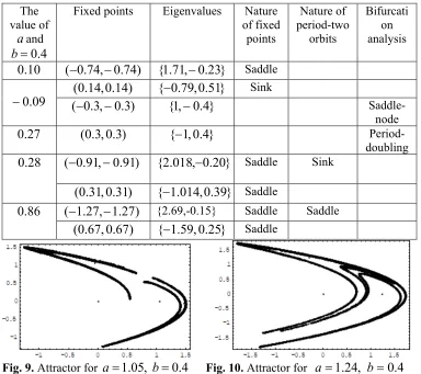
we can show the following results for the different values of parameter a from the calculations made in the following table by using Mathematica.(i) If the parameter values
0
.
09
<
a
<
0
.
27
,
b
=
0
.
4
,
the Hénon mapf
a,b will have one sink fixed point and one saddle fixed point.(ii) If the parameters value
a
=
−
0
.
09
,
b
=
0
.
4
,
a saddle-node bifurcation will occur. (iii) If the parameters valuea
=
0
.
27
,
b
=
0
.
4
,
a period-doubling bifurcation occurs when the fixed point loses stability and a period-two orbit is born.(iv) If the parameter values
0
.
27
<
a
<
0
.
85
,
b
=
0
.
4
,
the Hénon mapf
a,b will have saddle fixed points and period-two orbits are sink.(v) If the parameter values
0
.
85
<
a
<
1
.
25
,
b
=
0
.
4
,
the Hénon mapf
a,b will have saddle fixed points and period-two orbits are also saddle.The value of
aand
4 . 0
= b
Fixed points Eigenvalues Nature of fixed
points
Nature of period-two
orbits
Bifurcati on analysis
10 .
0
(
−
0
.
74
,
−
0
.
74
)
{
1
.
71
,
−
0
.
23
}
Saddle09 . 0
−
(
(
−
0
0
.
14
.
3
,
,
−
0
.
0
14
.
3
)
)
{
−
{
0
1
.
,
79
−
0
,
0
.
4
.
51
}
}
SinkSaddle-node 27
.
0
(
0
.
3
,
0
.
3
)
{
−
1
,
0
.
4
}
Period-doubling 28
.
0
(
−
0
.
91
,
−
0
.
91
)
{
2
.
018
,
−
0
.
20
}
Saddle Sink)
31
.
0
,
31
.
0
(
{
−
1
.
014
,
0
.
39
}
Saddle86 .
0
(
−
1
.
27
,
−
1
.
27
)
{2.69,-0.15} Saddle Saddle)
67
.
0
,
67
.
0
(
{
−
1
.
59
,
0
.
25
}
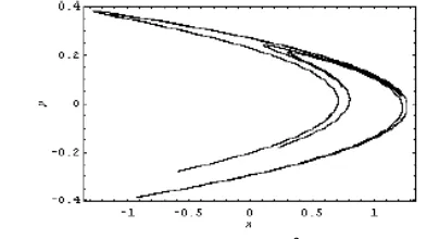
SaddleAbove Fig. 9 has two-pieces attractor for
a
=
1
.
045
,
b
=
0
.
4
.
The points of an orbit alternate between the pieces. In the Fig. 10, two-pieces have merged to form one-piece attractor fora
=
1
.
24
,
b
=
0
.
4
.
4.5. For the parameter value
b
=
0
.
3
,
we can show the following results for the different values of parameter a from the calculations made in the following table by using Mathematica.(i) If the parameter values
0
.
12
<
a
<
0
.
37
,
b
=
0
.
3
,
the Hénon mapf
a,b will have one sink fixed point and one saddle fixed point.(ii) If the parameters value
a
=
0
.
37
,
b
=
0
.
3
a period-doubling bifurcation occurs when the fixed point loses stability and a period-two orbit is born.(iii) If the parameter values
0
.
37
<
a
<
0
.
92
,
b
=
0
.
3
,
the Hénon mapf
a,b will have saddle fixed points and a period-two orbit is sink.(iv) If the parameter values
0
.
91
<
a
<
1
.
41
,
b
=
0
.
3
,
the Hénon mapf
a,b will have saddle fixed points and period-two orbits are also saddle.The value of
a and 3 . 0
= b
Fixed points Eigenvalues Nature of fixed points
Nature of
period-two orbits
Bifurcation analysis
13 .
0
(
−
0
.
85
,
−
0
.
85
)
{
1
.
86
,
−
0
.
16
}
Saddle)
15
.
0
,
15
.
0
(
{
−
0
.
72
,
0
.
42
}
Sink37 .
0
(
0
.
35
,
0
.
35
)
{
−
1
,
0
.
3
}
Period-doubling 91
.
0
(
−
1
.
37
,
−
1
.
37
)
{
2
.
85
,
−
0
.
11
}
Saddle Sink)
66
.
0
,
66
.
0
(
{
−
1
.
52
,
0
.
20
}
Saddle40 .
1
(
−
1
.
58
,
−
1
.
58
)
{
3
.
25
,
−
0
.
09
}
Saddle Saddle)
88
.
0
,
88
.
0
(
{
−
1
.
91
,
0
.
15
}
Saddle
Md. Jahurul Islam, Md. Shahidul Islam and M. A. Rahman
174
Above Fig. 11 has two-pieces attractor for
a
=
1
.
14
,
b
=
0
.
3
.
The points of an orbit alternate between the pieces. In the Fig. 12, two-pieces have merged to form one-piece attractor fora
=
1
.
4
,
b
=
0
.
3
.
4.6. For the parameter value
b
=
0
.
2
,
we can show the following results for the different values of parameter a from the calculations made in the following table by using Mathematica.(i) If the parameter values
0
.
16
<
a
<
0
.
48
,
b
=
0
.
2
,
the Hénon mapf
a,b will have one sink fixed point and one saddle fixed point.(ii) If the parameters value
a
=
−
0
.
16
,
b
=
0
.
2
,
a saddle-node bifurcation will occur. (iii) If the parameters valuea
=
0
.
48
,
b
=
0
.
2
,
a period-doubling bifurcation occurs when the fixed point loses stability and a period-two orbit is born.(iv) If the parameter values
0
.
48
<
a
<
1
.
01
,
b
=
0
.
2
,
the Hénon mapf
a,b will have a saddle fixed point and a period-two orbit sinks.(v) If the parameter values
1
.
00
<
a
<
1
.
62
,
b
=
0
.
2
,
the Hénon mapf
a,b will have saddle fixed points and a period-two orbit is also a saddle.The value of
a and 2 . 0
= b
Fixed points Eigenvalues Nature of fixed points
Nature of
period-two orbits
Bifurcation analysis
16 . 0
−
(
−
0
.
4
,
−
0
.
4
)
{
1
,
−
0
.
2
}
Saddle-node 17
.
0
(
−
0
.
97
,
−
0
.
97
)
{
2
.
04
,
−
0
.
09
}
Saddle)
17
.
0
,
17
.
0
(
{
−
0
.
65
,
0
.
31
}
Sink48 .
0
(
0
.
4
,
0
.
4
)
{
−
1
,
0
.
2
}
Period-doubling 99
.
0
(
−
1
.
47
,
−
1
.
47
)
{
3
.
01
,
−
0
.
07
}
Saddle Sink)
67
.
0
,
67
.
0
(
{
−
1
.
47
,
0
.
14
}
Saddle61 .
1
(
−
1
.
73
,
−
1
.
73
)
{
3
.
52
,
−
0
.
06
}
Saddle Saddle)
93
.
0
,
93
.
0
(
{
−
1
.
96
,
0
.
10
}
SaddleAbove Fig. 13 has two-pieces attractor for
a
=
1
.
26
,
b
=
0
.
2
.
The points of an orbit alternate between the pieces. In the Fig. 14, two-pieces have merged to form one-piece attractor fora
=
1
.
61
,
b
=
0
.
2
.
4.7. For the parameter value
b
=
0
.
1
,
we can show the following results for the different values of parameter a from the calculations made in the following table by using Mathematica.(i) If the parameter values
0
.
20
<
a
<
0
.
61
,
b
=
0
.
1
,
the Hénon mapf
a,b will have one sink fixed point and one saddle fixed point.(ii) If the parameters value
a
=
0
.
61
,
b
=
0
.
1
,
a period-doubling bifurcation occurs when the fixed point loses stability and a period-two orbit is born.(iii) If the parameter values
0
.
61
<
a
<
1
.
44
,
b
=
0
.
1
,
the Hénon mapf
a,b will have saddle fixed points and a period-two orbit is sink.(iv) If the parameter values
1
.
13
<
a
<
1
.
81
,
b
=
0
.
1
,
the Hénon mapf
a,b will have saddle fixed points and a period-two orbit is also a saddle.The value of
a and 1 . 0
= b
Fixed points Eigenvalues Nature of fixed points
Nature of
period-two orbits
Bifurcation analysis
60 .
0
(
−
1
.
34
,
−
1
.
34
)
{
2
.
72
,
−
0
.
04
}
Saddle)
44
.
0
,
44
.
0
(
{
−
0
.
98
,
0
.
10
}
Sink61 .
0
(
0
.
45
,
0
.
45
)
{
−
1
,
0
.
1
}
Period-doubling 12
.
1
(
−
1
.
47
,
−
1
.
47
)
{
3
.
01
,
−
0
.
07
}
Saddle Sink)
7
.
0
,
7
.
0
(
{
−
1
.
47
,
0
.
07
}
Saddle80 .
1
(
−
1
.
86
,
−
1
.
86
)
{
3
.
74
,
−
0
.
03
}
Saddle Saddle)
96
.
0
,
96
.
0
(
{
−
1
.
97
,
0
.
05
}
Saddle
Md. Jahurul Islam, Md. Shahidul Islam and M. A. Rahman
176
Above Fig. 15 has two-pieces attractor for
a
=
1
.
40
,
b
=
0
.
1
.
The points of an orbit alternate between the pieces. In the Fig. 16, two-pieces have merged to form one-piece attractor fora
=
1
.
80
,
b
=
0
.
1
.
5. Conclusion
From the above study we can conclude our result as follows:
(i) The Henon map
f
a,b has attractors with the parameter values.
1
|
|
and
2
1
<
<
<
−
a
b
In those attractor, four one-pieces attractors are found with the parameter values1
<
a
<
2
and
|
b
|
<
1
.
(ii) The Hénon map
f
a,b has two fixed points and period-two orbits which arecalled saddle with the parameter values
0
.
85
<
a
<
2
and
|
b
|
<
1
.
(iii) For the parameters values
a
=
0
.
12
,
b
=
0
.
6
;
a
=
0
.
19
,
b
=
0
.
5
;
;
4
.
0
,
27
.
0
=
=
b
a
a
=
0
.
37
,
b
=
0
.
3
;
a
=
0
.
48
,
b
=
0
.
2
;
anda
=
0
.
61
,
b
=
0
.
1
,
a period-doubling bifurcation occurs when the fixed point loses stability and a period-two orbit is born.(iv) The Hénon map is chaotic on the square whose side length 2 for the parameter values
a
>
0
and
|
b
|
<
1
.
REFERENCES
1. K. T. Alligood, Tim D. Sauer and James A. Yorke, Chaos. An Introduction to Dynamical Systems. New York, 1996.
2. R. L. Devaney, An Introduction to Chaotic Dynamical Systems, (2nd edn.). Addison-Wesley, Redwood City, 1989.
3. E. N. Lorenz, Deterministic Nonperiodic Flow, Journal of the Atmospheric Sciences, 20 (1963), 130 – 141.
4. Grassberger, P. and I. Procaccia, Measuring the Strangeness of Strange Attractors, Physica 9D, (1983), 189 – 208.
5. M. Hénon, A Two-dimensional Mapping with a Strange Attractor, Comm. Math. Phys., 50 (1976), 69 – 77.