Graph Coloring Using Linear Algebra
Tommy Rene Jensen
Kyungpook National University, Daegu, South Korea
Date Submitted: May 22, 2014 Originality: 95%
Date Revised: December 19, 2015 Plagiarism Detection: Passed
ABSTRACT
The classical problem in Combinatorics and Graph Theory of coloring the vertices of a given graph properly using a prescribed number of colors, is considered. This paper describes an application of elementary linear algebra over a finite field of order q to this problem, where q is the number of available colors.
INTRODUCTION
When a set of objects is required to become partitioned into classes, while imposing certain restrictions on which elements may or may not be allowed together in a class, the situation is commonly described formally as a problem of coloring the vertices (or edges) of a graph. With the vertices of a graph representing elements to be partitioned, and the colors representing the partition classes, an edge joining two vertices represents a prohibition against including the corresponding elements into the same class.
Both topics of coloring and edge-coloring are main research areas in Graph Theory, and each features a wealth of unsolved questions (Jensen and Toft, 1995 ;Jensen and Toft 2015).
Inspired by classical works of Tutte [5, 6], this paper studies the application of algebraic methods to graph coloring. The approach is more algorithmic than in Tutte’s papers, and applies matrices and elementary linear algebra in a novel way. Notation and Terminology
Let 𝐺 = (𝑉, 𝐸) be a finite graph with vertex set 𝑉and edge set 𝐸, possibly
containing multiple edges. A
function 𝜑 = 𝑉 → 𝐶 is a (proper) coloring
of 𝐺 if 𝜑(𝑢) ≠ 𝜑(𝑣) holds for every edge 𝑒 ∈ 𝐸 having 𝑢 and 𝑣 as its endvertices. In other words, any two adjacent vertices are required to be colored differently. If 𝑘 is the number of elements in 𝐶, then such a 𝜑 is a 𝑘-coloring.
Similarly a function 𝜓 ∶ 𝐸 → 𝐶 is a (proper) edge-coloring of 𝐺 if 𝜓(𝑒) ≠ 𝜓(𝑒′) holds for all distinct edges 𝑒 and 𝑒′
of 𝐺 that share a common end vertex , and 𝜓 is a 𝑘-egde-coloring 𝑘 = |𝐶|.
The finite field of order q is referred to as 𝔽𝑞. The set of all functions from a set 𝑋
to 𝔽𝑞 is denoted by 𝔽𝑞𝑋. If A and B are any
sets, and 𝑚 ∈ 𝔽𝑞𝐴×𝐵 is any function from
𝐴 × 𝐵 to 𝔽𝑞, we identify 𝑚 with a
Matrix 𝑀 is identified as having entries in 𝔽𝑞, so that the rows of 𝑀 are indexed by
the elements of 𝐴, and the columns are indexed by the elements of 𝐵. In particular the row of 𝑀 indexed by 𝑎 ∈ 𝐴 may be
identified with the function 𝑚𝑎∈ 𝔽𝑞𝐵
which maps 𝑏 to 𝑚(𝑎, 𝑏), for all ∈ 𝐵 , and similarly the column indexed by 𝑏 ∈ 𝐵corresponds to the function 𝑚𝑏 ∈ 𝔽𝑞𝐴
such that 𝑚𝑏(𝑎) = 𝑚(𝑎, 𝑏), for all 𝑎 ∈ 𝐴.
𝐴.
Let 𝐺 be any graph and assume that the
vertices of 𝐺 are numbered 𝑉 =
{𝑣1, 𝑣2, … , 𝑣𝑚}. Let 𝑀(𝐺) be the matrix
with entries in 𝔽𝑞 such that its rows are
indexed by 𝑉 and its columns by 𝐸, and such that if the ends of any edge 𝑒 are 𝑣𝑖
and 𝑣𝑗 with 𝑖 < 𝑗, then the column indexed
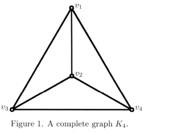
by 𝑒contains the entry 1 in row 𝑖, the entry −1 in row 𝑗 and zeroes in the entries of all other rows. For 𝐾4with the numbering of its
vertices shown in figure 1, the
corresponding matrix is
The row space 𝑅𝑆(𝑀) of 𝑀 is the vector space over 𝔽𝑞 generated by the set
of rows. That is,
𝑅𝑆(𝑀) = {∑ 𝛼(𝑎)𝑚𝑎∶ 𝛼 ∈ 𝑎∈𝐴
𝔽𝑞𝐴}.
Graph Coloring Explained in Matrix l Language
For positive integer 𝑛, a graph is a
complete graph 𝐾𝑛 if its vertex set has 𝑛
elements, and any two vertices are joined by precisely one edge. Thus the graph in figure 1 is a 𝐾4.
𝑀(𝐾4) =
[
1 1
−1 0
0 0
−1 0
1 0
0 1
0 −1
−1 0
0 0
1 0
0 −1
1 −1
] ,
when its rows are ordered according to the indices of the vertices, and its columns are
arranged from left to right
lexicographically.
The following observation is easily made. Observation. Let 𝐺 = (𝑉, 𝐸) be any graph and let 𝑐 ∶ 𝑉 → 𝔽𝑞 be any
function. Then 𝑐 is a coloring of 𝐺 if and
only if the element 𝑐𝑀(𝐺) =
∑𝑣∈ 𝑉𝑐(𝑣)𝑚𝑣 of the row space of 𝑀(𝐺)
Indeed, if 𝑒 is any edge of 𝐺, say, with endvertices 𝑣𝑖 and 𝑣𝑗, where 𝑖 < 𝑗,
then the coordinate entry of 𝑐𝑀(𝐺) corresponding to 𝑒 is ∑𝑣∈ 𝑉𝑐(𝑣)𝑚𝑣(𝑒) =
𝑐(𝑣𝑖) − 𝑐(𝑣𝑗), which is nonzero if and only
if 𝑐 assigns different values to 𝑣𝑖and 𝑣𝑗.
It is convenient to use the concept of weight for any vector 𝑥⃗ = (𝑥1, 𝑥2, … , 𝑥𝑛), defined by
𝑤(𝑣⃗) = |{𝑖 ∶ 𝑥𝑖 ≠ 0, 1 ≤ 𝑖 ≤ 𝑛}|,
so that the weight of 𝑥⃗ is equal to the number of nonzero coordinate values for 𝑥⃗. Call a vector heavy if its weight is the same as its dimension, that is, it contains no zero entries. A matrix is called heavy if its row space is empty or contains a heavy vector.
We deduce the following
equivalence.
Proposition 1. There exist a q-coloring of 𝐺 if and only if 𝑀(𝐺) is heavy.
The row space of a matrix does not change when applying elementary row operations:
(a) interchange of rows,
(b) multiplication of a row by a nonzero scalar,
(c) addition of a row to a different row, and
(d) removal of a row which consists entirely of zeroes.
In addition, the property of being heavy clearly does not change when applying
(e) interchange of columns,
(f) multiplication of a column by a nonzero scalar, and
(g) removal of a column which is identical to another column.
By combining (f) and (g) any column which is parallel to another column is simply deleted. From Proposition 1 we then get the following.
Proposition 2. There exists a q-coloring of 𝐺 if and only if it is possible to obtain a heavy matrix from 𝑀(𝐺) by repeated application of operations (a) – (g).
In the example of the graph 𝐾4, the
addition to the first row of the sum of all rows below it, followed by discarding the resulting all-zero row, multiplication of the resulting new first row by −1, and finally multiplication of each of the columns except the first and last by −1, produces a matrix in reduced row echelon form, that is, a matrix for which its initial columns form an identity submatrix of full row rank.
𝑀 = [ 1 0 0 1 0 0
0 1 0 1 1 0
1 0
0 1
1 −1 ] .
We note that this expression for 𝑀 is independent of the value of 𝑞, though if 𝑞 is even, then the −1 of the last column can be changed to positive 1.
Suppose that the row space of 𝑀 contains a heavy element, obtained as a linear combination of the three rows of 𝑀 by scalars 𝑎1, 𝑎2, 𝑎3 ∈ 𝔽𝑞, so that the 𝑖th
row from above is multiplied by
𝑎𝑖 and the resulting row vectors are added
𝑎1, 𝑎2, 𝑎3≠ 0
The fourth column imposes the condition
𝑎1+ 𝑎2≠ 0
Then 𝑞 = 2 results in a
contradiction, since 𝑎1, 𝑎2≠ 0 implies
𝑎1= 𝑎2= 1, and then 𝑎1+ 𝑎2= 1 +
1 = 0 follows by addition in 𝔽2. Thus we
deduce in passing that the graph 𝐾4does not
allow a 2-coloring. In fact the first, second and the fourth columns of 𝑀 arise from the triangle of vertices 𝑣1, 𝑣2, 𝑣3 in 𝐾4, and it is
clear that no 2-coloring of a triangle is possible.
Assume 𝑞 = 3. Then the condition that all of 𝑎1, 𝑎2, 𝑎1+ 𝑎2 are nonzero
implies that 𝑎1 and 𝑎2are both nonzero and
not the negatives of each other. Since the distinct elements of 𝔽3 are 0, −1, +1, it
follows that 𝑎1 and 𝑎2are either both −1 or
+1. In particular 𝑎1 = 𝑎2 holds. Then the
linear combination of the initial two rows of 𝑀 with coefficients 𝑎1, 𝑎2 is obtained
from the sum of the two rows by multiplying it by the scalar 𝑎1= 𝑎2.
Hence in the place of 𝑀 a matrix can be considered in which the first row is the sum of the two top rows of 𝑀. Applying operations (f, g) to remove redundant columns, we obtain the matrix, can be obtained.
𝑀′ = [1 0 0 1
1 1
1 −1] ,
which has the property that 𝑀 is heavy if and only if the same is true for 𝑀′. Repeating this argument for the two rows 𝑀′, using the conditions on their coefficients imposed by the three initial columns in order to produce a heavy
element of the row space, we consider the matrix obtained by adding the two rows: 𝑀′′= [1 1 −1 0] .Since every
element of the row space 𝑀′′ has its fourth entry equal to zero, it can be concluded that 𝑀′′is not heavy, and therefore no 3-coloring of 𝐾4 exists.
Assuming 𝑞 = 4, the desired linear combination of the rows of 𝑀 obtained by choosing as coefficients the three nonzero elements of 𝔽4, and we obtain the
conclusion is obtained that a 4-coloring of 𝐾4 does exist.
Instead of evoking an ad hoc argument as in the case of 𝑞 = 4, an additional operation to deal with this case more elegantly is introduced. Call a vector
light if its weight is strictly less than q. then the operation is considered by deleting (h) the columns that correspond to the nonzero entries of a light element of the row space.
Theorem 3. There exists a q-coloring of 𝐺 if and only if a heavy matrix can be obtained from 𝑀(𝐺) by applying a sequence of operations (a) – (h).
Proof. It is clear that the deletion of any columns from a heavy matrix produces another heavy matrix. In particular, if all columns are deleted, this follows from the fact that a matrix with empty row space is heavy, by definition. Hence by Proposition 2, it is enough to prove that
operation (h) preserves the property of not being a heavy matrix.
columns of 𝑋 in which the entries of 𝑥⃗ are nonzero, and let 𝑌 be the matrix obtained from 𝑋 by deleting these columns from 𝑋. It is assumed that 𝑌 is heavy, and that 𝑋 is also heavy. Have to be shown if the row space of 𝑌 is empty, then 𝑥⃗ is already a heavy element of the row space of X, so it is done. Now it can be assumed that the row space of 𝑌 contains a heavy element 𝑦⃗.
Let 𝑟1, 𝑟2, … , 𝑟𝑛 be the rows of 𝑋
and 𝑠1, 𝑠2, … , 𝑠𝑛 be the rows of 𝑌 in the
corresponding order. Assume that 𝑦⃗ is the linear combination 𝑦⃗ = ∑𝑛𝑖=1𝑎𝑖𝑠𝑖 of the
rows of 𝑌, and let 𝓏⃗ be the corresponding element 𝓏⃗ = ∑𝑛𝑖=1𝑎𝑖𝑟𝑖 of the row space of
𝑋. Then the 𝑛 − 𝑤 coordinate values of the entries of 𝓏⃗ which correspond to columns of 𝑌 are identical to the corresponding values in 𝑦⃗, hence they are also nonzero, since 𝑦⃗ is heavy. But in columns of 𝓏⃗ indexed by 𝑊 there will possibly appear zeroes.
For each 𝜆 ∈ 𝔽𝑞, let 𝓏⃗𝜆= 𝓏⃗ +
𝜆𝑥⃗. Then 𝓏⃗𝜆is an element of the row space
of 𝑋 which has the same coordinate values as 𝓏⃗ in the entries that correspond to column of 𝑌, hence these are nonzeroes. There remain the 𝑤 coordinate places in the columns 𝑊 for which the entries of 𝓏⃗𝜆can
possibly be zero. For any fixed column 𝑗 ∈ 𝑊, the q vectors 𝓏⃗𝜆(𝜆 ∈ 𝔽𝑞) have values
in entry 𝑗 that are obtained by adding all different multiples of the nonzero entry 𝑗 of 𝑥⃗ to the entry 𝑗 of 𝓏⃗. Hence these values are all different. It follows that for each fixed column in 𝑊, there is precisely one of the 𝓏⃗𝜆 which has a zero in entry 𝑗. Using the
pigeonhole principle, there exists λ0∈ 𝔽𝑞
such that 𝓏⃗𝜆0 has no zero value in any
column 𝑊. Hence 𝓏⃗𝜆0 is heavy, and it
follows that 𝑋 is heavy.
We observe that to determine whether a matrix with 𝑛 rows which is given in reduced row echelon form contains a light element in its roe space, and to find one if it exists, it is enough to inspect only the fewer than (𝑛𝑞)𝑞−1 row space elements that are linear combinations of 𝑞 − 1rows. This is since an element that cannot be obtained in this way clearly has weight at least q.
Now, since all rows of the matrix 𝑀(𝐾4) are light for 𝑞 = 4, we readily
deduce from Theorem 3 that the graph, unsurprisingly, is 4-colorable.
An Approach to 3-Coloring
In this section we concentrate on the special case 𝑞 = 3. We already observed that if matrix is in reduced row echelon form, then the following operation may be performed, making the new matrix heavy if and only if this is the cease for the original.
(h) (𝑞 = 3) if a column contains precisely two nonzero entries, and these are
equal, then delete the two
corresponding rows and replace them by their sum.
More generally, if any three columns of a matrix are linearly dependent, and no two of them are parallel, then the matrix is brought into
We observed that three linearly independent and mutually non-parallel columns of the matrix 𝑀(𝐺) of a graph 𝐺 correspond to the three edges of a triangle in 𝐺, that is, three pairwise adjacent vertices.
To answer the question of whether a given matrix 𝑀 with entries in 𝔽3 is
heavy, we can attempt the following stepwise procedure.
STEP 0 Let the current matrix be the input matrix 𝑀.
STEP 1 If the current matrix has a column with all its entries equal to zero, then STOP and output ‘NO’.
STEP 2 (i) apply (f) and (g) to obtain a matrix without parallel columns.
(ii) If the current matrix has three linearly dependent columns, then apply (b) and (c) to obtain a matrix in which two of these columns have exactly one nonzero entry, and the nonzero entries of the third are equal. Apply (i) to this matrix, then go to STEP 1.
STEP 3 (i) Apply (a) – (d) to obtain a matrix in reduced row echelon form. (ii) If the row space of the current matrix
has a light element, apply (h).
(iii) If the current matrix has no columns, then STOP and output ‘YES’.
(iv) Repeat STEP 3.
This procedure is not ensured to halt. In STEP 3 it is possible that there are no light elements in the row space of the current matrix, in which case STEP 3 gets repeated indefinitely. In view of the fact that the decision problem of 3-colorability of a graph is NP-complete, see [4], this is no surprise. Each step is executable in polynomial time, hence if the procedure always produces a modified matrix having fewer rows or columns in every step, then it would be describe a polynomial algorithm for an NP-complete problem, thus showing P = NP, which is generally considered unlikely to hold true.
However, on a positive note, the question of 3-edge-coloring of 3-regular graphs is briefly considered. The Petersen graph𝑃10 shown in Figure 2 is the smallest
example of s snark, a 3-regular graph that nontrivially does not allow such a coloring.
The appropriate matrix for
reformulating this question into a linear algebra setting is the line graph matrix
𝑀𝐿(𝐺) over the field 𝔽3. Its rows are
distinct edges that share a common end vertex, with nonzero entries of the column only in the two rows labeled by 𝑒1 and 𝑒2,
one entry a +1, the other a −1. In the case of the Petersen graph, such a matrix has 15 rows and 30 columns.
It is noteworthy that in literature there are few if any proofs given of the fact that the Petersen graph does not allow a 3-edge-coloring which does not apply symmetry considerations or case checking. The reader is invited to apply the above procedure to the matrix 𝑀 = 𝑀𝐿(𝑃10) to
obtain a proof which uses only
straightforward calculations, and neither
symmetry considerations nor case
checking.
CONCLUSION
The stepwise procedure described in the previous section is easily modified to give a backtracking algorithm, which for any input graph will produce the correct answer to the question of whether a 3-coloring exists. Whenever STEP 3(ii) fails to reduce the current matrix, the algorithm could branch into two possibilities; for some two rows either to replace them both by their sum, or to replace then both by their difference. Then STEP 1 would be replaced by a backtracking step in case no coloring can be found, unless no further backtracking is possible and the algorithm halts with a negative answer.
It is also straightforward with a little more bookkeeping to produce an actual coloring of the graph in the case when the procedure is able to decide that one exists.
A more detailed analysis of a generalized method of applying matrices to graph coloring, from a perspective of Matroid Theory, may be found in the unpublished manuscript (Jensen, 2001).
REFERENCES
Jensen, T.R., application of linear
matroids to deciding graph
colorability, Hamburger Beitäge zur
Mathematik, #123, 2001.
Preprint.math.umihamburg.de/publi c//papers/hbm/hbm2001123.ps.gz
Jensen, T.R., and Toft, B., Graph Coloring Problems, Wiley 1995.
Jensen, T.R., and Toft, B., Unsolved Graph Colouring Problems, in
Topics in Chromatic Graph Theory, eds. L. Beineke and R. Wilson, Cambridge University Press, 2015.
Garey, M.R., and Johnson, D.S.,
Computers and Intractability: A guide to the theory of NP-Completeness. W. H. Freeman 1979.
W.T Tutte, A contribution to the theory of chromatic polynomials, Canad. J. Math. 6 (1954), 80-91