R E S E A R C H
Open Access
Estimation of exposure to toxic releases using
spatial interaction modeling
Jamison F Conley
Abstract
Background:The United States Environmental Protection Agency’s Toxic Release Inventory (TRI) data are frequently used to estimate a community’s exposure to pollution. However, this estimation process often uses underdeveloped geographic theory. Spatial interaction modeling provides a more realistic approach to this estimation process. This paper uses four sets of data: lung cancer age-adjusted mortality rates from the years 1990 through 2006 inclusive from the National Cancer Institute’s Surveillance Epidemiology and End Results (SEER) database, TRI releases of carcinogens from 1987 to 1996, covariates associated with lung cancer, and the EPA’s Risk-Screening Environmental Indicators (RSEI) model.
Results:The impact of the volume of carcinogenic TRI releases on each county’s lung cancer mortality rates was calculated using six spatial interaction functions (containment, buffer, power decay, exponential decay, quadratic decay, and RSEI estimates) and evaluated with four multivariate regression methods (linear, generalized linear, spatial lag, and spatial error). Akaike Information Criterion values andPvalues of spatial interaction terms were computed. The impacts calculated from the interaction models were also mapped. Buffer and quadratic interaction functions had the lowest AIC values (22298 and 22525 respectively), although the gains from including the spatial interaction terms were diminished with spatial error and spatial lag regression.
Conclusions:The use of different methods for estimating the spatial risk posed by pollution from TRI sites can give different results about the impact of those sites on health outcomes. The most reliable estimates did not always come from the most complex methods.
Background
Environmental pollution data such as that collected by
the United States Environmental Protection Agency’s
Toxic Release Inventory (TRI) have been used exten-sively for studies in environmental justice and medical geography [1]. These studies involved estimating an individual’s or a community’s exposure to pollution using the spatial information contained in the TRI data-base. Despite the use of this spatial information, the geographical theory used to guide the estimation of location-based exposure to pollution has frequently been limited to basic containment and buffer analysis, espe-cially at the national scale. The aim of this research is to improve the spatial analysis of TRI data by incorporat-ing distance decay effects derived from spatial interac-tion modeling in order to provide a more realistic
approach to the estimation of location-based exposure to pollution, particularly airborne pollution. This is achieved by using several different functions for calcu-lating this exposure and comparing the results when they are used in multivariate regression analyses with lung cancer mortality rates.
The different methods for estimating the risk at a location are evaluated because, while many studies have explored and demonstrated a link between environmen-tal pollution and a variety of adverse socieenvironmen-tal and medi-cal effects [1], understanding the nature of this relationship is equally important. As the variety of meth-ods used to estimate these impacts attests, the nature of this relationship is not as well understood as the exis-tence of the relationship. The form of this relationship greatly impacts the answers to questions that may arise from the discovery of a relationship, such as the extent to which rural counties experience adverse impacts from urban polluters. A visual cartographic comparison of
Correspondence: [email protected]
Department of Geology and Geography, West Virginia University, 330 Brooks Hall, 98 Beechurst Ave., Morgantown, WV, USA, 26506
some approaches has been explored by McMaster et al [2], although they do not make the statistical compari-son carried out here.
Prior work
Spatial analyses of toxic pollution data, whether for environmental justice or for medical geography, have typically used a simple spatial estimate of exposure. The exposure has been recorded as a binary variable (exposed or not exposed) either through spatial contain-ment such that a person is exposed if they live in the same census tract or county as an industrial site [1,3-8], or a spatial buffer such that a person is exposed if they live within a threshold distance (e.g., 1 mile) of an industrial site [5,9-12]. Variations on the latter use mul-tiple buffers to approximate decreasing risk with increased distance, or select a small number of neigh-borhoods at increasing distances which can be treated as samples from multiple buffers. This enables the study to reflect decreased exposure as the distance increases [1,9,13-15]. To provide a better measure of the impact of sites on a census tract, four studies [16-19] use a ras-ter grid that can account for whether a site is in the center of the tract, or near an edge, and whether any sites are just over the border in neighboring tracts. These raster grids reflect the density of TRI sites around each raster cell, although the density is calculated using a small buffer, such as the density of sites within a one mile radius of the cell. A gradual decay of impact as dis-tance increases is still lacking.
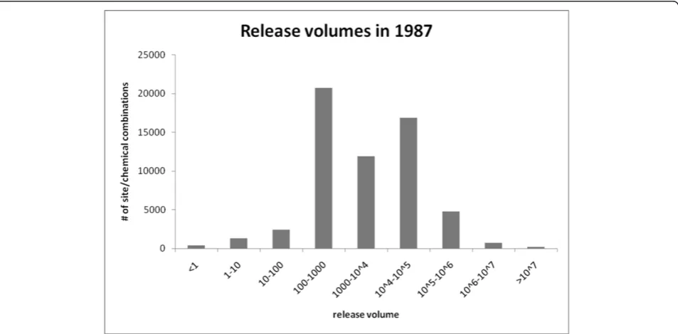
Accounting for the volume of the release is another important factor missed by some TRI studies [6,10,16,18]. A binary approach that considers all TRI sites equally does not allow for gradients of risk, treats exposure to one site as equivalent to exposure to many sites, and does not account for the volume and toxicity of releases at each site. The release volumes vary by orders of magnitude (figure 1). Recognizing this, many researchers do account for varying release volumes from each site [7,9,12,20-27]. They often use variations of the spatial containment and buffer models described above which can incorporate the release volume (equations 1 and 2 respectively). Here,kijis the impact of siteion countyj,tiis the volume of releases at sitei,dijis the distance between siteiand countyj, and
Tis the threshold distance. As a result of this, most studies that use these techniques to account for the release volume still reflect a simple treatment of geography by not including distance decay effects. The toxic impacts of the different chemicals on human health vary as well [3,9,12,22-25,27], although this variation is not addressed in the current study.
kij=
ti:i⊂j
0 : o.w. (1)
kij=
ti:dijT
0 : o.w. (2)
To address these simplifying assumptions, Dent et al [26] have proposed using a GIS to combine atmospheric
modeling with the release data and health outcomes and provide a detailed analysis of the potential effects and risks associated with TRI releases. Morello-Frosch et al [23,24] and Fisher et al [21] similarly incorporate atmo-spheric modeling in their analysis. These models are typically used for local, rather than national-scale analy-sis. The United States Environmental Protection Agency’s Risk-Screening Environmental Indicators (RSEI) Model uses principles of atmospheric modeling to derive a level of risk across the entire United States [28]. This has been used by Abel [9] and Downey and Hawkins [27], and is used in this resesarch.
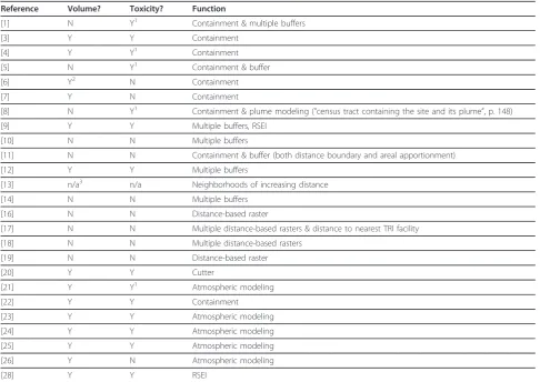
This background discussion is summarized by table 1, which shows that while distance decay approaches have been used, e.g. [20], containment and buffers are the most common with atmospheric modeling becoming more prevalent in local studies. Exponential and power-based distance decay approaches as found in spatial
interaction modeling have, to the author’s knowledge, not been used at all.
Spatial interaction modeling
In this research, I use a spatial interaction modeling approach that is more flexible than the binary approaches commonly used in spatial analysis of TRI data, yet is fast enough and generic enough to apply to the thousands or millions of release sites involved in a national scale study. Spatial interaction modeling was developed in economic geography to estimate the level of economic interaction between two towns [29-32]. The underlying assumptions are analogous to the phy-sics theory of gravity. Just as two objects in space exert a stronger gravitational pull on each other as they increase in size and move closer to each other, two towns are expected to have a stronger level of eco-nomic interaction as the towns increase in size and as Table 1 Prior work summary
Reference Volume? Toxicity? Function
[1] N Y1 Containment & multiple buffers
[3] Y Y Containment
[4] Y Y1 Containment
[5] N Y1 Containment & buffer
[6] Y2 N Containment
[7] Y N Containment
[8] N Y1 Containment & plume modeling ("census tract containing the site and its plume”, p. 148)
[9] Y Y Multiple buffers, RSEI
[10] N N Multiple buffers
[11] N N Containment & buffer (both distance boundary and areal apportionment)
[12] Y Y Multiple buffers
[13] n/a3 n/a Neighborhoods of increasing distance
[14] N N Multiple buffers
[16] N N Distance-based raster
[17] N N Multiple distance-based rasters & distance to nearest TRI facility
[18] N N Multiple distance-based rasters
[19] N N Distance-based raster
[20] Y Y Cutter
[21] Y Y1 Atmospheric modeling
[22] Y Y Containment
[23] Y Y Atmospheric modeling
[24] Y Y Atmospheric modeling
[25] Y Y Atmospheric modeling
[26] Y N Atmospheric modeling
[28] Y Y RSEI
Papers summarized by the type of spatial interaction method applied and whether toxicity and the release volume are accounted for in the analysis.
1
Analyzes one or more classes of chemicals separately.
2
Incorporates number of releases, but not volume.
3
the distance between them decreases. These broad trends are applicable in many fields within geography, even though the specific functional form from physics (equation 3), may not be as useful as other functional forms.
These models are used to estimate the effect of each TRI site on each county. As the toxic release volume increases, the impact of that site on the county increases. Likewise, the impact of nearby sites is assumed to be greater than the impact of more distant sites, as from Tobler’s First Law of Geography [33].
There are two common distance decay functions used to model spatial interaction, which control the rate at which the impact of a site decreases with distance. The first, taken from the physics model of gravity, is the power equation, in which the impact of a site is tional to the size of the release and inversely propor-tional to the distance raised to a parameterized exponent (equation 3). Here,a andθare positive con-stant parameters. The location of a county is given by its centroid. Because other functional forms may be more applicable than the gravitational form, exponential decay functions (equation 4) have also been developed and used.
kij=tiαd−θij (3)
kij=tiαexp
−θdij
(4)
The models in economic geography, such as those in Sen and Smith [31], give equations with a third term which in this work corresponds to the population of the county and a related positive constant b, such that the power model becomes kij=tiαpiβd−θij and the exponen-tial model becomes kij=tiapbiexp(-θdij). Because I use age-adjusted rates of lung cancer rather than unadjusted counts for the dependent variable, these population terms are set to 1 and effectively removed from the equations.
The only application of a distance decay function to TRI data is a comparison of toxic releases and federally assisted housing which uses a quadratic distance decay function [20] (equation 5). This is referred to here as the Cutter function after the lead author of the publica-tion in which it was first proposed. It uses a constant parameter, θ, controlling the rate of decrease, and a threshold distance beyond which the impact is zero. The equation given here modifies equation 1 from Cut-ter et al [18] to incorporate the volume of the release. As in the other equations,kij is the impact of sitei on countyj, ti is the volume of releases at sitei, dij is the
distance between site i and county j, and T is the
threshold distance.
kij=tiα
1.0− dij
θ
Tθ
(5)
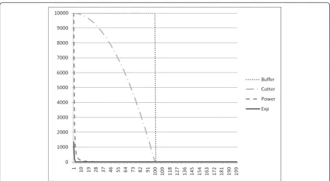
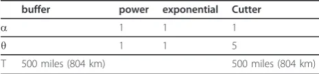
Figure 2 shows the effect of increasing distance on all the models except the containment model. The para-meters of the models shown are 1.0 fora, 2.0 forθ, and 100 for T, with a release volume of 10,000. More com-plex atmospheric models, which can incorporate dis-tance decay concepts, have been used predominantly in studies at a local scale [21,23,24,26], with only the RSEI dataset used at the national scale [27].
Methods Data used
Four sets of data are used in this paper. The first are lung cancer age-adjusted mortality rates from the National Cancer Institute’s Surveillance Epidemiology and End Results (SEER) database [34]. These rates are from the years 1990 through 2006 inclusive. The sec-ond are TRI releases from 1987 to 1996. The years chosen for the TRI databases reflect a lag time between chronic exposure to toxic chemicals and the development of lung cancer. All data are temporally aggregated to the entire time series, rather than evalu-ating year-by-year temporal lags. The third are risk
estimates computed by the EPA’s RSEI program to be
used as a basis for comparison against the spatial interaction estimates The RSEI data are the risk-related results calculated from airborne releases of che-micals that are flagged as carcinogenic and have a non-zero Inhalation Unit Risk.
designation from the Appalachian Regional commission which overlaps parts of the northeast, Midwest and southern regions. Due to a lack of data, information regarding personal movements is not included, although analysis comparing place of birth with place of death may partially account for this [39].
The Modifiable Areal Unit Problem [40] introduces difficulties into the interpretation at the county scale, especially in the larger counties in the western United States where the county centroid may be tens of miles away from the county’s population center. Additionally, in these larger counties, the risk may vary within the county, and this variance is masked by calculating the risk at the county scale. However, some of the covariate data (e.g., the BRFSS-derived smoking rate) is not avail-able at a finer scale, necessitating a county-level analysis. In the research presented here, the impacts of the Modi-fiable Areal Unit Problem and large county sizes are expected to have a similar impact across all models because all tests use the same spatial scale.
An examination using a synthetic dataset was consid-ered, but the results of such a test would minimize the AIC in the situation reflecting the way the dataset is constructed (e.g., the impact falls off according to an exponential distance decay function), which may or may not correspond to a real world situation. Therefore,
actual, rather than synthetic, data are used in this research.
Methods Applied
Three sets of releases from 1987 to 1996 in the TRI database are used. The first is all releases flagged as car-cinogenic. The second is all releases of chemicals identi-fied as inducing lung cancer. These chemicals are those from a parallel study [41] plus beryllium and lead, which were identified as related to lung cancer by the lead author of [41] in a private communication. The total list of chemicals is arsenic, beryllium, 1,3-buta-diene, cadmium, chromium, formaldehyde, lead and nickel. The third set of releases adds to the second set those releases identified as generic compound categories of elements in the first set. An example of this is a release of“arsenic compounds”in addition to releases of plain arsenic. The impacts of these three sets of releases on all counties in the contiguous United States were cal-culated using the containment, buffer, power, exponen-tial and Cutter models given above. These release impacts are summed to create the cumulative impact on a county (equation 6), where kij is the impact of site i on countyjand Kjis the cumulative impact on county
j. Because the release amounts vary by several orders of magnitude and have an approximately lognormal
distribution, as shown in figure 1, both the log10 -trans-formed and the untrans-trans-formed release volumes were tested.
Kj=
i
kij (6)
The calculated impacts and covariates are then used in multivariate regression models calculated with the R software package [42]: ordinary least squares (OLS) lin-ear regression, general linlin-ear model regression (GLM), spatial lag regression, and spatial error regression. The latter two incorporate spatial dependence in the regres-sion model and are detailed below. There is spatial auto-correlation in the response variable (Moran’s I = 0.69, p < 0.01), demonstrating the existence of spatial depen-dence and suggesting the applicability of the spatial regression techniques. Geographically Weighted Regres-sion [40], which can vary the regresRegres-sion coefficients across the study area was not applied because it is unli-kely that the nature of the relationship between toxic releases and mortality changes across the country.
This situation is not strictly one of evaluating a single function against a null hypothesis of zero impact from toxic emissions, but is rather evaluating many different functions against both each other and the null hypoth-esis. This makes the task more akin to model parameter optimization than traditional statistical hypothesis test-ing. It is considered here that, of the different functions and their parameterizations, the most appropriate repre-sentation is the one that minimizes the Akaike Informa-tion Criterion (AIC) of a regression test in which the modeled risk is one of the independent variables. In all the regression tests used in this comparison, the remain-der of the independent variables are the demographic, behavioral and regional covariates, and the dependent variable is lung cancer mortality.
Experiments testing many parameterizations of the buffer, Cutter, power, and exponential functions were used to guide the results given here. These parameteri-zations are for the contiguous United States, and were evaluated on which parameterizations gave the lowest AIC values when combined with the covariate data in an OLS regression using the lung cancer mortality rate as the dependent variable. The same tests are conducted for the containment and RSEI approaches to risk esti-mation for comparison. AIC values were also computed for generalized linear model regressions, although none of the generalized linear model regressions produced lower AIC values than linear regression. As a result, the generalized linear model regressions are not further dis-cussed. Preliminary experiments (not presented) demon-strated that the parameterizations that perform well for OLS regression also typically perform well for the spatial
lag and spatial error regressions. The tests presented here evaluateaand θvalues of 1.0, 1.5, 2.0, 2.5, 3.0, 3.5, 4.0, 4.5, and 5.0, and distance thresholds of 5, 10, 15, ... 500 miles (8, 16, 24, ... 805 km) for the buffer and Cut-ter functions. AfCut-ter the parameCut-terizations were found, spatial lag regression and spatial error regression models were computed. Also, linear regression models for each of the rural-urban continuum codes from the United States Department of Agriculture. Lastly, maps of pro-portion of the TRI impact for each county that origi-nated in release sites located in urban areas were produced. This allows an examination of whether the impact of sites in urban areas is limited to those cities, or whether it extends far into the surrounding rural areas, and demonstrates that some environmental justice questions are not robust to the choice of risk model.
Spatial Regression Methods
The two spatial regression methods, spatial lag and spa-tial error regression, both account for the spaspa-tial auto-correlation that is almost always present in geographic data by adding a term to the regression equation. This spatial autocorrelation can be the result of diffusion effects of the dependent variable, which is unlikely in this situation, or the result of risk factors which have not been accounted for elsewhere in the regression model inducing spatial autocorrelation of the dependent variable [43]. The standard OLS regression (equation 7) estimates the dependent variable, which is the lung can-cer mortality rate, as a linear combination of the inde-pendent variables, here the TRI interaction term and the demographic covariates. The county is j, the dependent variable at county jisYj, the independent variables at county j are Xj,a,εjis the error term, andb0 ... bnare the regression coefficients.
Yj=β0+ n
a=1
βaXj,a+εj (7)
Spatial lag regression incorporates the autocorrelation directly into the model by including a term where the dependent variable at countyjis dependent not only on the independent variables at county j, but also on the dependent variable values of countyj’s neighbors [44].
The neighbors are defined by a weights matrix typically using one of the following three options: (1) all counties which share a border with countyjas its neighbors, (2) all counties within a threshold distance of countyjas its
neighbors, or (3) the nearest neighbors of county j.
and Utah) as neighbors, which is called“queen contigu-ity”to assess the sensitivity of the results to the choice of weights matrix. Thus spatial lag regression uses the dependent variable values of the neighbor counties to calculate a new independent variable for countyj, giving
equation 8, where r is a coefficient describing the
strength of the spatial autocorrelation,wj,k is the spatial weight between countiesj andk(typically 1 for neigh-bors and 0 for non-neighneigh-bors, but a distance decay form for the weights is possible), and Njis the neighborhood of counties around county j. The r coefficient can be
estimated in the same way that the b coefficients are
estimated. A computationally efficient approach is given in Smirnov and Anselin [45].
Yj=β0+ n
a=1
βaXj,a+ρ
k∈Nj
wj,kYk+εj (8)
Spatial error regression (equation 9) works similarly to spatial lag regression, except the autocorrelation term applies to the error terms of the neighboring counties rather than their dependent variable values [46]. Because of the circular dependence of the error terms (ie, if county jis in county k’s neighborhood and vice versa,
the value of εj is affected by the value of εk while the value ofεk is affected by the value of εj), standard esti-mation techniques will not work. An estiesti-mation proce-dure for this is also given by Smirnov and Anselin [45].
Yj=β0+ n
a=1
βaXj,a+λ
k∈Nj
wj,kεk+εj (9)
Results
Table 2 presents the parameterizations that gave the lowest AIC values and thus are used for further analysis. The results shown use the lung carcinogens with com-pounds dataset. All three TRI release sets described above (all carcinogens, lung carcinogens, lung carcino-gens with compounds) were evaluated as were the log10 transformed release values, and the lung carcinogens and related compounds gave the lowest overall AIC values. While the containment approach was best fit with the log-transformed releases of lung carcinogens and related compounds, and the exponential and power
functions had the best fits with releases of all carcino-gens, the improvements were minimal; the differences in AIC are less than 2.0 for containment and the exponen-tial function and approximately 10.0 for the power func-tion. Therefore, to ensure consistency in the later tables, the untransformed releases of lung compounds with car-cinogens are used.
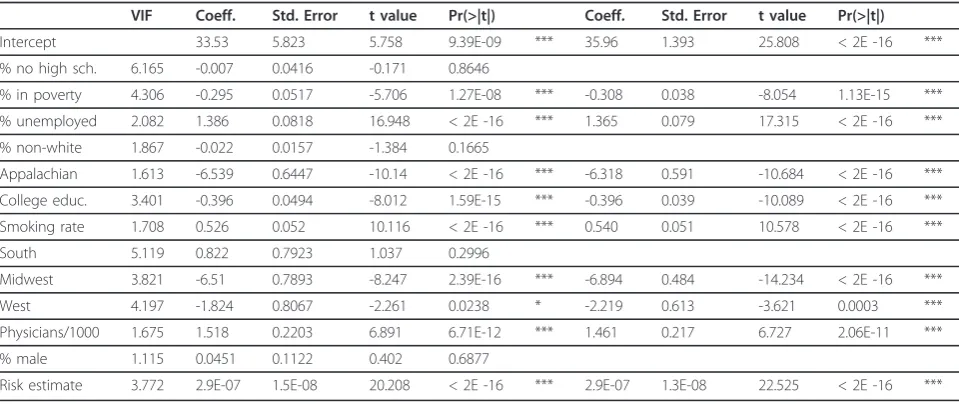
Table 3 shows the R-squared values, the Akaike Infor-mation Criterion, and the probabilities that the spatial interaction terms are non-zero. For each regression model (OLS, spatial lag, or spatial error), the best-per-forming distance decay function is highlighted in bold. In all cases, this was the buffer model. Table S1 in Addi-tional file 1 shows the equivalent table for the queen contiguity weights matrix. The choice of weights matrix did not alter the results for most decay functions, only substantially increasing the AIC of the buffer model, but not enough to make another decay function better. As such, the change in weights matrix did not alter conclu-sions about which decay function performed best. Table 4 gives the full regression results for the overall best parameterization: the buffer model at 500 miles (804 km). This table also gives values of each indepen-dent variable’s variance inflation factor (VIF). Since all the VIFs are less than 10, collinearity is not problematic in this model. As some of the covariates did not have significant coefficients in the best-performing model, the least significant covariate was iteratively removed from the model until all independent variables were signifi-cant, producing the model in the right side of table 4. Similarly, non-linear functions of each of the indepen-dent variables were also applied to each of the six para-meterizations in Table 3, following [47]. While the fits are improved (minimized AIC = 22126.54 with the buf-fer function), the more complex regression models do not alter the conclusions about which spatial interaction models perform well and which perform poorly. Table S2 in Additional file 2 gives the best performing model results. Table 5 gives the R-squared values of the OLS regressions by urban-rural code. The values of these codes are in table 6.
Maps of the percent of TRI impact in each county that is due to source locations in urban counties according to each of the distance decay functions are given in figure 3. The buffer, Cutter, exponential and power functions using the parameterizations in table 2 are shown. The darker counties have a greater percent of their impact from releases in urban counties, whether the total impact is high or low.
Discussion
The buffer and Cutter functions outperform the con-tainment, power and exponential functions (Table 3). This improvement is notable both for the R-squared Table 2 Model parameterizations
buffer power exponential Cutter
a 1 1 1
θ 1 1 5
T 500 miles (804 km) 500 miles (804 km)
values of the OLS regressions and the Akaike Infor-mation Criterion (AIC) for all regressions. Because the AIC penalizes regression models with more para-meters, lower values are preferred. These functions also outperformed the RSEI risk-related results values, which was not the expected outcome. Other RSEI pro-ducts, the hazard, modeled hazard, and modeled hazard*population product were also tested, but all performed worse than the buffer and Cutter functions. However, the power and exponential functions from the spatial interaction literature did not perform much better than leaving out the toxicity term, and occa-sionally even increased the AIC value, which may result from the coarse resolution of the county-level dataset. These two functions may yet be useful at a finer scale.
The improvement of the buffer and Cutter functions over the RSEI data demonstrates that despite the diffi-culties posed by the Modifiable Areal Unit Problem and the size of large western counties obscuring variation of risk within the county, these spatial interaction approaches may still be an accurate reflection of the risks posed by TRI facilities. It should be cautioned that while this work demonstrates a relationship between TRI facilities and lung cancer, it does not yet indicate a causal link, nor does it indicate that the best-fitting risk estimation method, a large buffer around the TRI site, has the strongest causal relationship with lung cancer mortality.
Additionally, AIC values are better for the spatial regression techniques compared to the OLS regression values. However, including the TRI term in the spatial
Table 4 OLS Regression results
VIF Coeff. Std. Error t value Pr(>|t|) Coeff. Std. Error t value Pr(>|t|)
Intercept 33.53 5.823 5.758 9.39E-09 *** 35.96 1.393 25.808 < 2E -16 ***
% no high sch. 6.165 -0.007 0.0416 -0.171 0.8646
% in poverty 4.306 -0.295 0.0517 -5.706 1.27E-08 *** -0.308 0.038 -8.054 1.13E-15 ***
% unemployed 2.082 1.386 0.0818 16.948 < 2E -16 *** 1.365 0.079 17.315 < 2E -16 ***
% non-white 1.867 -0.022 0.0157 -1.384 0.1665
Appalachian 1.613 -6.539 0.6447 -10.14 < 2E -16 *** -6.318 0.591 -10.684 < 2E -16 ***
College educ. 3.401 -0.396 0.0494 -8.012 1.59E-15 *** -0.396 0.039 -10.089 < 2E -16 ***
Smoking rate 1.708 0.526 0.052 10.116 < 2E -16 *** 0.540 0.051 10.578 < 2E -16 ***
South 5.119 0.822 0.7923 1.037 0.2996
Midwest 3.821 -6.51 0.7893 -8.247 2.39E-16 *** -6.894 0.484 -14.234 < 2E -16 ***
West 4.197 -1.824 0.8067 -2.261 0.0238 * -2.219 0.613 -3.621 0.0003 ***
Physicians/1000 1.675 1.518 0.2203 6.891 6.71E-12 *** 1.461 0.217 6.727 2.06E-11 ***
% male 1.115 0.0451 0.1122 0.402 0.6877
Risk estimate 3.772 2.9E-07 1.5E-08 20.208 < 2E -16 *** 2.9E-07 1.3E-08 22.525 < 2E -16 ***
Results for the multivariate ordinary least squares regression of age-adjusted lung cancer mortality versus covariates and risk estimates from lung carcinogens and related compounds calculated with the buffer model. This is shown as it minimizes the AIC across all decay functions (Table 3).
Significance codes: 0.0001‘***’0.001‘**’0.01‘*’. n = 3057.
Table 3 Regression results
OLS no term contain. buffer power exp. Cutter RSEI
R-squared 0.4596 0.46 0.5224 0.4623 0.4596 0.5178 0.4599
Akaike Info. Criterion 22873.61 22873.22 22498.13 22860.47 22875.59 22527.45 22874.03 probability of TRI term n/a 0.122677 <.000001 0.000104 0.877151 <.000001 0.209438 Spatial Lag
Akaike Info. Criterion 22875.6 22875.21 22350.12 22852.86 22876.37 22529.4 22876.02 probability of TRI term n/a 0.91113 <.000001 0.96198 0.91903 0.83221 0.9158 Spatial Error
Akaike Info. Criterion 22873.95 22873.51 22298.14 22850.64 22874.72 22525.14 22874.57 probability of TRI term n/a 0.19085 <.000001 0.13587 0.19759 0.038097 0.22659
regression techniques does not lead to as much improvement over the base case of no interaction term. Even so, the improvement in the buffer model gives the spatial error regression of the buffer model the lowest AIC value. Both the Moran’s I spatial autocorrelation statistic given above and the lower AIC values for the spatial regression techniques indicate that there is spa-tial dependence in lung cancer mortality. Moreover, this spatial dependence is not accounted for by the
independent variables. This dependence is most likely the result of one or more additional spatial processes affecting lung cancer that are not accounted for in these data, rather than a simple diffusion or contagion process of lung cancer itself. The limited improvement from adding the TRI impacts strengthens the suggestion that there remain geographic processes affecting lung cancer that are not accounted for in these datasets. While it is not executed in this study, GWR may also reveal further evidence of confounding processes by revealing interac-tions with modeled covariates via non-stationary regres-sion coefficients.
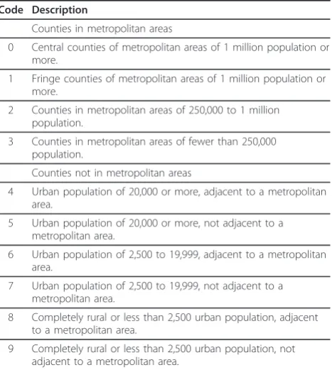
As with the different regression methods, the buffer and Cutter functions have the best R-squared values across the entire range of rural-urban continuum codes (Table 5). Also, category 5, defined as counties contain-ing a larger town (more than 20,000 residents) but which are not adjacent to a metropolitan area, has much higher R-squared values than the other rural-urban codes across all models. It is not yet clear why this would be the case.
These results suggest that changing the method used to estimate risk will change the representation of the spatial impacts of the TRI sites on public health. As others have noted, the scope and scale of analysis can substantially impact the results [48], so researchers should be cautious when generalizing these findings at a county scale and national scope to more local scales and scopes. Nonetheless, researchers using the TRI dataset to estimate the health risks from pollution should care-fully consider the method used to estimate the risk, as the most sophisticated model used here, the RSEI data, did not provide the lowest AIC values.
The maps in figure 3 display the percent of the TRI impact on each county from sources in urban areas cal-culated using the functions that performed best in the earlier results. As estimated by these models, the poten-tial effects of pollution from urban TRI releases extend far beyond the limits of the urban areas. However, the extent varies depending on which function is used and how it is parameterized, highlighting the importance of using an appropriate function. In the power and expo-nential maps (figure 3a and 3b), the impacts from urban release sites are more limited to urban areas and the nearby rural communities. In both the buffer and Cutter maps (figure 3c and 3d), rural areas in the northeastern and southwestern United States, have between 75 and 100% of their estimated TRI impact from release sites in urban areas. These extended effects of urban areas are related to the large radii used in the distance decay functions. Additional work is needed to examine the environmental toxicology to determine whether the che-micals being released could travel such large distances or whether these models are simply capturing spatial Table 6 Definition of each rural-urban code
Code Description
Counties in metropolitan areas
0 Central counties of metropolitan areas of 1 million population or more.
1 Fringe counties of metropolitan areas of 1 million population or more.
2 Counties in metropolitan areas of 250,000 to 1 million population.
3 Counties in metropolitan areas of fewer than 250,000 population.
Counties not in metropolitan areas
4 Urban population of 20,000 or more, adjacent to a metropolitan area.
5 Urban population of 20,000 or more, not adjacent to a metropolitan area.
6 Urban population of 2,500 to 19,999, adjacent to a metropolitan area.
7 Urban population of 2,500 to 19,999, not adjacent to a metropolitan area.
8 Completely rural or less than 2,500 urban population, adjacent to a metropolitan area.
9 Completely rural or less than 2,500 urban population, not adjacent to a metropolitan area.
The interpretation of each 1993 rural-urban continuum code used in Table 5. Table 5 OLS regression R-squared values by rural-urban code
Code no term contain. buffer Cutter exp. power
0 0.4971 0.4971 0.5682 0.5493 0.5100 0.4978 1 0.4113 0.4318 0.4795 0.4840 0.4119 0.4345 2 0.4654 0.4655 0.5143 0.5065 0.4655 0.4690 3 0.4618 0.4678 0.5216 0.5089 0.4621 0.4660 4 0.4815 0.4818 0.5514 0.5210 0.4828 0.4841 5 0.5886 0.5905 0.6753 0.6425 0.5899 0.5939 6 0.3990 0.3992 0.4562 0.4436 0.3997 0.3990 7 0.5231 0.5231 0.5882 0.5862 0.5234 0.5232 8 0.5555 0.5628 0.5829 0.5749 0.5560 0.5578 9 0.5741 0.5746 0.5892 0.5909 0.5748 0.5764
dependence of the outcome that is induced by a con-founding spatial process.
Future work will investigate the parameterization choices of the functions. This ad hoc approach to para-meterization-examining different possibilities of thea,θ and threshold parameters-is not the ideal approach. Sta-tistical approaches to finding the optimala andθ para-meters can be incorporated to improve the spatial interaction models that are generated [29,30,32]. A geos-tatistical approach can be applied to determine the decay function form and parameters. A correlogram plot comparing the distance between two counties and the difference between their mortality rates or their resi-duals from a regression function could be used to para-meterize the function. Additionally, subsets of the
correlogram could be examined separately to investigate anisotropy and non-stationarity. However, with both the ad hoc approach in this paper and a statistical model-fit-ting approach, using the data to optimize the parameters and then using those parameters to analyze the same data introduces circularity into the model-fitting process that would best be avoided.
A more theoretically sound approach would be to vary
theaand θparameters based on the properties of the
toxic chemicals that are released. Varyingais similar to methods used somewhat frequently to account for the dif-ferent toxicity of the chemicals released [2,8,11,20-22], although the studies cited here use multiplicative rather than exponential modifiers (atiinstead oftia). In each
case, higher values of a correspond to more toxic
chemicals. Different studies have made this adjustment using different references, including American Conference of Governmental Industrial Hygienists Threshold Limit Values [3,22], a chronic toxicity index [12], an inhalation unit risk [23], a lifetime cancer risk [24], and the RSEI model [9,27]. Similarly,θandTcan be varied to reflect differences in airborne transport of the chemicals. If a che-mical travels more easily and farther, lower values ofθand higher values ofTcan be used. These parameters can also be varied based on the direction from the release site to the affected community, thus incorporating anisotropy.
Ongoing work includes the refinement of at-risk population estimates using the LandScan USA popula-tion dataset [49] which can explore variapopula-tion missed by county-level populations unable to capture fine-scale risks. For example, if a chemical is only present in the atmosphere within a mile of the release site, any county-by-county analysis will be problematic because the spatial resolution of county-level data are coarser than a square mile. The LandScan dataset provides population estimates at a 3 arc-second resolution (roughly 90 meters). This can then provide improved estimates of the number of people within one mile of the release site instead of assigning the impact of a release site on the county as if everybody lived at the centroid of the county. This approach will have stronger effects on the power and exponential models because they have more rapid decreases in the impact as one travels farther from the release site (figure 2). This ongoing work also incorporates the adjustments given above varying the parameters to account for properties of the chemicals released and local climatic conditions to account for prevailing wind directions.
Conclusions
The research in this paper demonstrates that the use of simple containment techniques for estimating the spatial risk posed by pollution from TRI sites as well as the RSEI risk-related results can give misleading results about the impact of those sites on health outcomes. This is done through a comparison of multivariate regression results using inputs of six different functions for estimating the impact of a release site on a county: containment, buffering, the quadratic distance decay function proposed by Cutter et al [20], an inverse power distance decay function, an exponential distance decay function, and the RSEI risk-related results. The buffer and Cutter approaches consistently performed the best among these methods. The effects of this function choice are also demonstrated through mapping the per-cent of the overall impact that comes from urban TRI sites for all models except containment. As refinements to the parameterization process are made, the utility of
more theoretically sound spatial interaction models will improve further.
Additional material
Additional file 1: Table S1 - Results for the multivariate ordinary least squares, spatial lag, and spatial error regressions of age-adjusted lung cancer mortality versus covariates and risk estimates from releases of lung carcinogens and related compounds calculated with each spatial interaction model. Spatial regressions here use queen contiguity matrix to determine whether two counties are neighbors. Bold entries indicate which spatial interaction model performed best. Note that lower values for the Akaike Information Criterion are preferred.
Additional file 2: Table S2 - Results for the multivariate ordinary least squares regression of age-adjusted lung cancer mortality versus nonlinear functions of both covariates and risk estimates from lung carcinogens and related compounds calculated with the buffer model. This is shown as it minimizes the AIC across all decay functions (Table 3). This is equivalent to Table 4 in the main document, but includes natural logarithms (e.g., log(pov)), squared values (e.g., pov2) and cubed values (e.g., pov3).
Acknowledgements
Support for this report was provided by the Office of Rural Health Policy, Health Resources and Services Administration, PHS Grant No. 1 U1CRH10664-01-00. The author also acknowledges Dr. Michael Hendryx for support and comments on an earlier draft of this manuscript. Lastly, the author thanks two anonymous referees for their valuable comments and suggestions.
Competing interests
The author declares that he has no competing interests.
Received: 14 September 2010 Accepted: 21 March 2011 Published: 21 March 2011
References
1. Pastor M Jr, Sadd JL, Morello-Frosch R:Waiting to Inhale: The Demographics of Toxic Air Release Facilities in 21st-Century California.
Soc Sci Quart2004,85:420-440.
2. McMaster RB, Leitner H, Sheppard E:GIS-based Environmental Equity and Risk Assessment: Methodological Problems and Prospects.Cart and Geog Info Sys1997,24:172-189.
3. Bowen WM, Salling MJ, Haynes KE, Cyran EJ:Toward Environmental Justice: Spatial Equity in Ohio and Cleveland.Annals of the Assn of Am Geog1995,85:641-663.
4. Cohen MJ:The spatial distribution of toxic chemical emissions: Implications for nonmetropolitan areas.Soc & Nat Res1997, 10:17-39.
5. Croen LA, Shaw GM, Sanbonmatsu L, Selvin S, Buffler PA:Maternal Residential Proximity to Hazardous Waste Sites and Risk for Selected Congenital Malformations.Epidemiology1997,8:347-354.
6. Cutter SL, Solecki WD:Setting environmental justice in space and place: Acute and chronic airborne toxic releases in the southeastern United States.Urb Geog1996,17:380-399.
7. Daniels G, Friedman S:Spatial Inequality and the Distribution of Industrial Toxic Releases: Evidence from the 1990 TRI.Soc Sci Quart1999, 80:244-262.
8. Shaw GM, Schulman J, Frisch JD, Cummins SK, Harris JA:Congenital Malformations and Birthweight in Areas with Potential Environmental Contamination.Arch of Env Health1992,47:147-154.
9. Abel TD:Skewed Riskscapes and Environmental Injustice: A Case Study of Metropolitan St. Louis.Env Mgmt2008,42:232-248.
11. Kearney G, Kiros GE:A spatial evaluation of socio demographics surrounding National Priorities List sites in Florida using a distance-based approach.Int J Health Geog2009,8:33.
12. Neumann CM, Forman DL, Rothlein JE:Hazard Screening of Chemical Releases and Environmental Equity Analysis of Populations Proximate to Toxic Release Inventory Facilities in Oregon.Env Health Persp1998, 106:217-226.
13. Berry M, Bove F:Birth Weight Reduction Associated with Residence near a Hazardous Waste Landfill.Env Health Persp1997,105:856-861. 14. Knox EG, Gilman EA:Hazard proximities of childhood cancers in Great
Britain from 1953-80.J Epid Comm Health1997,51:151-159.
15. Nordström S, Beckman L, Nordenson I:Occupational and environmental risks in and around a smelter in northern Sweden: I. Variations in birth weight.Hereditas1978,88:43-46.
16. Downey L:Spatial Measurement, Geography, and Urban Racial Inequality.Social Forces2003,81:937-952.
17. Mennis J:Using Geographic Information Systems to Create and Analyze Statistical Surfaces of Population and Risk for Environmental Justice Analysis.Soc Sci Quart2002,83:281-297.
18. Mohai P, Saha R:Reassessing racial and socioeconomic disparities in environmental justice research.Demography2006,43:383-399. 19. Mennis JL, Jordan L:The Distribution of Environmental Equity: Exploring
Spatial Nonstationarity in Multivariate Models of Air Toxic Releases.
Annals of the Assn of Am Geog2005,95:249-268.
20. Cutter SL, Hodgson ME, Dow K:Subsidized Inequities: The Spatial Patterning of Environmental Risks and Federally Assisted Housing.Urb Geog2001,22:29-53.
21. Fisher JB, Kelly M, Romm J:Scales of environmental justice: Combining GIS and spatial analysis for air toxics in West Oakland, California.Health & Place2006,12:701-714.
22. Horvath A, Hendrickson CT, Lave LB, McMichael FC, Wu TS:Toxic Emissions Indices for Green Design and Inventory.Env Sci & Tech1996,29:86A-90A. 23. Morello-Frosch R, Pastor M Jr, Sadd J:Environmental justice and Southern
California’s‘riskscape’.Urb Affairs Rev2001,36:551-578.
24. Morello-Frosch R, Pastor M Jr, Porras C, Sadd J:Environmental Justice and Regional Inequality in Southern California: Implications for Future Research.Env Health Persp2002,110:149-154.
25. Pastor M Jr, Morello-Frosch R, Sadd JL:Breathless: Schools, Air Toxics, and Environmental Justice in California.The Policy Studies J2006,34:337-362. 26. Dent AL, Fowler DA, Kaplan BM, Zarus GM, Henriques WD:Using GIS to
Study the Health Impact of Air Emissions.Drug and Chem Toxic2000, 23:161-178.
27. Downey L, Hawkins B:Single-Mother Families and Air Pollution: A National Study.Soc Sci Quart2008,89:523-536.
28. United States Environmental Protection Agency:Risk-Screening Environmental Indicators (RSEI) Model.[http://www.epa.gov/opptintr/rsei/]. 29. Batty M, Mackie S:The calibration of gravity, entropy, and related models
of spatial interaction.Env and Planning1972,4:205-233.
30. Baxter M:Estimation and inference in spatial interaction models.Prog Human Geog1983,7:40-59.
31. Sen A, Smith TE:Gravity Models of Spatial Interaction BehaviorNew York, NY: Springer; 1995.
32. Sheppard ES:The distance-decay gravity model debate.InSpatial Statistics and Models.Edited by: Gaile GL, Willmott CJ. Boston, MA: D. Reidel Publishing Company; 1984:367-388.
33. Tobler WR:A computer movie simulating urban growth in the Detroit region.Econ Geog1970,46:234-240.
34. SEER. Surveillance, Epidemiology, and End Results (SEER) Program: SEER*Stat Database: Incidence - SEER 13 Regs Limited-Use. Nov 2009 Sub (1992-2007) <Katrina/Rita Population Adjustment>.National Cancer Institute, Cancer Statistics Branch, released April 2010, based on the November 2009 submission; [http://www.seer.cancer.gov].
35. ARF:Area Resource FileRockville, MD: 2006 U.S. Department of Health and Human Services, Health Resources and Services Administration, Bureau of Health Professions; 2005.
36. Thun MJ, Henley SJ, Burns D, Jemal A, Shanks TG, Calle EE:Lung Cancer Death Rates in Lifelong Nonsmokers.J of Natl Cancer Inst2006, 98:691-699.
37. Blot WJ, Fraumeni JF Jr:Geographic Patterns of Lung Cancer: Industrial Correlations.Am J Epidem1976,103:539-550.
38. Hendryx M, O’Donnell K, Horn K:Lung Cancer Mortality Is Elevated in Coal-Mining Areas of Appalachia.Lung Cancer2008,62:1-7. 39. Sabel CE, Boyle PJ, Löytönen M, Gatrell AC, Jokelainen M, Flowerdew R,
Maasilta P:Spatial Clustering of Amyotrophic Lateral Sclerosis in Finland at Place of Birth and Place of Death.Am J Epidem2003,157:898-905. 40. O’Sullivan D, Unwin DJ:Geographic Information Analysis.2 edition. Hoboken,
NJ, USA: John Wiley & Sons, Inc; 2010.
41. Luo J, Hendryx M, Ducataman A:Association between Six Environmental Chemicals and Lung Cancer Incidence in the United States.J Rural Health, in review.
42. The R Project:The R Project for Statistical Computing. [http://www.r-project.org/].
43. Ward MD, Gleditsch KS:Spatial Regression ModelsLos Angeles, CA, USA: Sage Publications; 2008.
44. Robert Haining:Spatial Data Analysis: Theory and PracticeCambridge, UK: Cambridge University Press; 2003.
45. Smirnov O, Anselin L:Fast maximum likelihood estimation of very large spatial autoregressive models: a characteristic polynomial approach.
Comput Stat & Data Anal2001,35:301-319.
46. Rogerson PA:Statistical Methods for Geography: A Student’s Guide.2 edition. Los Angeles, CA, USA: Sage Publications; 2006.
47. Austin MP, Belbin L, Meyers JA, Doherty MD, Luoto M:Evaluation of statistical models used for predicting plant species distributions: Role of artificial data and theory.Ecol Model2006,199:197-216.
48. Baden BM, Noonan DS, Turaga RMR:Scales of Justice: Is there a Geographic Bias in Environmental Equity Analysis?J Env Plan Mgmt2007, 50:163-185.
49. Bhaduri B, Bright E, Coleman P, Urban M:LandScan USA: A High Resolution Geospatial and Temporal Modeling Approach for Population Distribution and Dynamics.GeoJournal2007,69:103-117.
doi:10.1186/1476-072X-10-20
Cite this article as:Conley:Estimation of exposure to toxic releases
using spatial interaction modeling.International Journal of Health Geographics201110:20.
Submit your next manuscript to BioMed Central and take full advantage of:
• Convenient online submission
• Thorough peer review
• No space constraints or color figure charges
• Immediate publication on acceptance
• Inclusion in PubMed, CAS, Scopus and Google Scholar
• Research which is freely available for redistribution