The Thirty-Third AAAI Conference on Artificial Intelligence (AAAI-19)
The Utility of Sparse Representations for Control in Reinforcement Learning
Vincent Liu,
1Raksha Kumaraswamy,
1Lei Le,
2Martha White
1 1Department of Computing Science, University of Alberta, Edmonton, Canada{vliu1, kumarasw, whitem}@ualberta.ca
2Department of Computer Science, Indiana University Bloomington, Indiana, USA [email protected]
Abstract
We investigate sparse representations for control in reinforce-ment learning. While these representations are widely used in computer vision, their prevalence in reinforcement learning is limited to sparse coding where extracting representations for new data can be computationally intensive. Here, we begin by demonstrating that learning a control policy incrementally with a representation from a standard neural network fails in classic control domains, whereas learning with a repre-sentation obtained from a neural network that has sparsity properties enforced is effective. We provide evidence that the reason for this is that the sparse representation provides local-ity, and so avoids catastrophic interference, and particularly keeps consistent, stable values for bootstrapping. We then dis-cuss how to learn such sparse representations. We explore the idea of Distributional Regularizers, where the activation of hidden nodes is encouraged to match a particular distribution that results in sparse activation across time. We identify a simple but effective way to obtain sparse representations, not afforded by previously proposed strategies, making it more practical for further investigation into sparse representations for reinforcement learning.
Introduction
Learning performance in artificial intelligence systems is highly dependent on the data representation—the features. An effective representation captures important attributes of the state (or instance), as well as simplifies the estimation of predictors. Consider a reinforcement learning agent. A local representation enables the agent to more feasibly make accurate predictions for that local region, because the local dy-namics are likely to be a simpler function than learning global dynamics. Additionally, such a representation can help pre-vent forgetting or interference (McCloskey and Cohen 1989; French 1991), by only updating local weights, as opposed to dense representations where any update would modify many weights. At the same time, it is important to have a distributed representation (Bengio 2009; Bengio, Courville, and Vincent 2013), where the representation for an input is distributed across multiple features or attributes, promoting generalization and a more compact representation.
Such properties can be well captured by sparse represen-tations: those for which only a few features are active for a
Copyright c2019, Association for the Advancement of Artificial
Intelligence (www.aaai.org). All rights reserved.
fully connected fully
connected x1
: x2
xn
fully
connected connectedfully y
SPARSE REPRESENTATION SUPERVISION
SIGNAL SPARSE REPRESENTATION NEURAL NETWORK
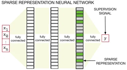
Figure 1: A neural network with dense connections produc-ing a sparse representation: Sparse Representation Neural Network (SR-NN). The green squares indicate active (non-zero) units, making a sparse last hidden layer where only a small percentage of units are active. This contrasts a network with sparse connections—which is often also called sparse. Sparse connections remove connections between nodes, but are likely to still produce a dense representation.
given input (Figure 1). Enforcing sparsity promotes identi-fying key attributes, because it encourages the input to be well-described by a small subset of attributes. Sparsity, then, promotes locality, because local inputs are likely to share sim-ilar attributes (simsim-ilar activation patterns) with less overlap to non-local inputs. In fact, many hand-crafted features are sparse representations, including tile coding (Sutton 1996; Sutton and Barto 1998), radial basis functions and sparse dis-tributed memory (Kanerva 1988; Ratitch and Precup 2004). Other useful properties of sparse representations—which can be seen as projecting data into a higher-dimensional space—include invariance (Goodfellow et al. 2009; Rifai et al. 2011); decorrelated features per instance (F¨oldi´ak 1990); improved computational efficiency for updating weights in the predictor, as only weights corresponding to active features need to be updates; and enabling linear separability in the high-dimensional space (Cover 1965), which facilitates the learning of a simple linear predictor. Further, such sparse, dis-tributed representations have been observed in the brain (Ol-shausen and Field 1997; Quian Quiroga and Kreiman 2010; Ahmad and Hawkins 2015).
and radial basis functions (Sutton and Barto 1998). They are effective for incremental learning, but can be difficult to scale to high-dimensional inputs because they grow expo-nentially with input dimension. Neural networks much more feasibly enable scaling to high-dimensional inputs, such as images, but can be problematic when used with incremental training. Instead, techniques like target networks, inspired by batch methods such as fitted Q-iteration (Riedmiller 2005), have been necessary for many of the successes of control with neural networks. We provide some evidence in this pa-per that this modification is necessary with dense, but not sparse, networks because the reinforcement learning agent bootstraps off its own estimates. If the value in other states are overwritten, the agent will bootstrap off inaccurate esti-mate. Local representations, however, are much less likely to suffer from interference and these issues with bootstrap-ping. Learned sparse representations, then, are a promising strategy to obtain the benefits of previously common, fixed sparse representations with the scaling of neural networks.
Learning sparse representations, however, does remain a challenge. There have been some approaches developed to learning sparse representations incrementally, particu-larly through factorization approaches for dictionary learn-ing (Mairal et al. 2009; 2010; Le, Kumaraswamy, and White 2017) or for general sparse distributions (Olshausen and Field 1997; Olshausen 2002; Teh et al. 2003; Ranzato et al. 2006; Ranzato, Boureau, and LeCun 2007; Lee et al. 2008), like Boltzmann machines. In sparse coding, for example, the sparse representation learning problem is formulated as a matrix factorization, where input instances are reconstructed using a sparse, or small subset, of a large dictionary. Many of the methods for general sparse distribution, however, are expensive or complex to train and those based on sparse coding have been found to have serious out-of-sample is-sues (Mairal et al. 2009; Lemme, Reinhart, and Steil 2012; Le, Kumaraswamy, and White 2017).
There are fewer methods using feedforward neural net-work architectures. Certain activation functions—such as linear threshold units (LTU) (McCulloch and Pitts 1943) and rectified linear units (ReLU) (Glorot, Bordes, and Ben-gio 2011)—naturally provide some level of sparsity, but of course provide no such guarantees. Early work on catas-trophic interference investigated some simple heuristics for encouraging sparsity, such as node sharpening (French 1991). Though catastrophic interference was reduced, the resulting networks were still quite dense.1 k-sparse auto-encoders (Makhzani and Frey 2013) use a top-k constraint per instance: only the topknodes with largest activations are kept, and the rest are zeroed. Winnner-Take-All auto-encoders (Makhzani and Frey 2015) use a k% response
con-1There have been strategies developed for catastrophic
interfer-ence that rely on rehearsal or dedicating subparts of the network to particular tasks. This work is a complementary direction for un-derstanding catastrophic interference for a sequential multi-task setting. We explore specifically the utility of sparse representations for alleviating interference for RL agents learning incrementally on one task, but do not necessarily imply that it is the only strategy to alleviate such interference. The comparisons in this work, therefore, focus on other strategies to learn sparse representations.
straint per node across instances, during training, to pro-mote sparse activations of the node over time. These ap-proaches, however, can be problematic—as we reaffirm in this work—because they tend to truncate non-negligible values or produce insufficiently sparse representations. An-other line of work has investigated learning or specifying sparse activation functions for neural networks (Triesch 2005; Ranzato et al. 2006; Lemme, Reinhart, and Steil 2012; Arpit et al. 2015), but used a sigmoid activation which is unlikely to result in sparse representations. They define spar-sity based on norms of the vector, rather than activation level. In this work, we first highlight that learned sparse represen-tations can significantly improve control performance, under an incremental learning setting, compared to dense neural networks. We visualize the activation of the hidden nodes for the sparse representation as well as the action-values for particular states. These provide evidence that locality helps avoid catastrophic interference and improves accuracy of action-values for bootstrapping. We then investigate a simple strategy for encouraging sparsity in neural networks: Dis-tributional Regularizers. This approach flexibly enables any desired architecture, simply with the addition of a KL diver-gence on the activation level for a node. We show that direct use of such a regularizer can cause dead filters or collapse— activation concentrating on a few nodes—potentially explain-ing why this simple strategy has not yet found wide-spread use. We show that a simple clipping is sufficient to obtain effective sparse representations, and conclude with a compar-ison to several other strategies for obtaining a sparse repre-sentation on the same benchmark domains.
Background
In reinforcement learning (RL), an agent interacts with its environment, receiving observations and selecting actions to maximize a reward signal. The environment is formalized by a Markov decision process (MDP), with statesS, actions
A, transition probabilities Pr:S × A × S →[0,1], rewards
R:S × A × S →Rand discount functionγ:S × A × S →
[0,1](White 2017).
One algorithm for on-policy control is Sarsa, where the agent updates its action-values for its current policy and acts near-greedily according to these values. The action-values for a policyπ:S × A →[0,1]are the expected return for that policy, starting from statesand actiona:
Qπ(s, a) =E[Gt|St=s, At=a] (1)
where,Gt=Rt+1+γt+1Gt+1
These action-values can be estimated with function approx-imation, such as with neural network. Because the expected return is a real-value target, such a neural network typically uses a linear activation on the last layer:
Qπ(s, a)≈Qˆw,θ(s, a) :=φθ(s, a)
>w (2)
wherew∈Rdis the weights in the last layer andφθ:S ×
A →Rdis therepresentationlearned by the network with
of the action-value approximation, therefore, relies on this representationφθ(s, a).
The Utility of Sparsity for Control
We begin by highlighting the utility of sparsity for control before discussing how to learn sparse representations. We show that two sparse representations—tile coding and sparse representation learned by a neural network (referred to as
SR-NNfrom hereon)—both significantly improve stability
in control. We choose tile coding, a static representation, as a baseline to compare to, as it known to perform very well in the benchmark RL domains we experiment with (Sutton and Barto 1998). We hypothesize that the main reason is due to catastrophic interference, which is much less problematic for the local representations typically provided by a sparse representations. We show both that SR-NN does appear to have more stable action-values for bootstrapping, and that the learned sparse representation is local, providing some evidence for this hypothesis.
We evaluate control performance on four benchmark do-mains: Mountain Car, Puddle World, Acrobot and Catcher. All domains are episodic, with discount set to 1 until ter-mination. We choose these domains because they are well-understood, and typically considered relatively simple. A pri-ori, it would be expected that a standard action-value method, like Sarsa, with a two-layer neural network, should be capable of learning a near-optimal policy in all four of these domains. We provide details about the domains in the Appendix.
The experimental set-up is as follows. To extract a repre-sentation with a neural network, to be used for control, we pre-train the neural network on a batch of data with a mean-squared temporal difference error (MSTDE) objective and the applicable regularization strategies. The training data con-sists of trajectories generated by a fixed policy that explores much of the space in the various domains. For the SR-NN, we use our distributional regularization strategy, described in a later section. This learned representation is then fixed, and used by a (fully incremental) Sarsa(0) agent for learn-ing a control policy, where only the weightswon the last layer are updated. The meta-parameters for the batch-trained neural network producing the representation and the Sarsa agent were swept in a wide range, and chosen based on con-trol performance. The aim is to provide the best opportunity for a regular feed-forward network (NN) to learn on these problems, as it is more sensitive to its meta-parameters than the SR-NN. Additional details on ranges and objectives are provided in the Appendix.
We choose this two-stage training regime to remove con-founding factors in difficulties of training neural networks incrementally. Our goal here is to identify if a sparse represen-tation can improve control performance, and if so, why. The networks are trained with an objective for learning values, on a large batch of data generated by a policy that covers the space; the learned representations are capable of represent-ing the optimal policy. We investigate their utility for fully incremental learning. Outside of this carefully controlled experiment, we advocate for learning the representation in-crementally, for the task faced by the agent.
Cumulative r
ewar
d
per episode
Mountain Car Puddle World Acrobot Catcher
-200
-600
50
100
50 50 100 50 100
-500
-1500
1000 500
Episode number
-100
-300 SR-NN
SR-NN
SR-NN
SR-NN TC
NN
TC
NN
TC
NN
TC
NN
Figure 2: Learning curves for Sarsa(0) comparing SR-NN, Tile Coding and vanilla NN in the four domains.
Cumulative r
ewar
d per episode
-100
-200
-300
0
-200
-400
0
-200
-400
-600
50
0 100
50 50 100
100
50 500 1000
SR-NN SR-NN
SR-NN
SR-NN Dropout NN
l1-NN
l2-NN
Dropout-NN
l2-NN
Dropout-NN l1-NN
l2-NN
Dropout-NN l1-NN
l2-NN
Mountain Car Puddle World
Acrobot Catcher
Episode number
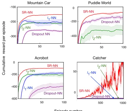
Figure 3: Learning curves for Sarsa(0) comparing SR-NN to the regularized representations. All representations except
`1-NN in Puddle World could reach goals more than 70 times
out of 100.`1does poorly in Puddle World, and is not visible.
The learning curves for the four domains, with Tile-Coding (TC), SR-NN and NN, are shown in Figure 2. Both SR-NN and NN used two-layers, of size[32,256], with ReLU activa-tions. The NNs performs surprisingly poorly, in some case increasing and then decreasing in performance (Mountain Car), and in others failing altogether (Catcher). In all the benchmark RL domains, the baseline sparse representation, TC, performs well, as expected. Specifically in Catcher, TC learns a close-to-optimal policy as the representation is pow-erful. The learned SR-NN performs as well in all domains, and is effective for learning in Catcher, whereas NN performs really poorly in all domains, and does not learn anything in Catcher. Both SR-NN and NN representations were trained in the same regime, with similar representational capabilities. Yet, the sparsity of SR-NN enables the Sarsa(0) agent to learn, where the regular feed-forward NN does not. We investigate this effect further in the next sets of experiments, to better understand the phenomenon.
To determine if the main impact of the sparse representa-tion is simply from regularizarepresenta-tion, preventing overfitting, we tested several regularization strategies for the neural network. These include`2and`1on the weights of the network (`2
-NN and`1-NN respectively) and Dropout on the activation
SR-NN l2-NN l1-NN Dropout-NN NN
Number of steps (x*103)
1 7 2 12 20 100 1 5 20 100
0
-15
-30
-50
-150
-250
0
-150
-300
0
-20
-40
0
-200
-600 Estimated
(s,a) value
0.0 0.32 0.135 0.139 0.0 0.12 0.0 1.25 0.0 1.6
True (s,a) value
0
-20
-40 : : : : :
c
b
d a
Figure 4: A study in Puddle World to investigate the effect of locality during on-policy control. (a) The activation maps for 20 randomly chosen neurons for different representations - each cell in the heatmap corresponds to the complete Puddle World state-space. The activation maps, and magnitude of activation of SR-NN are visibly sparser, and lower, when compared to Dropout and NN.`1and`2are quite dense in terms of activation area, whereas the magnitudes are really low - due to regularization of
the network weights. (b) A visualization of the domain, denoting the selected state-action pairs used in the analysis. (c) The estimated state-action values for the selected configurations during on-policy control with Sarsa(0) (= 0.1), while utilizing the specific representation of interest. (Sarsa(0) budget - 100 episodes with 1k episode cut-off for all representations). (d) The true state-action values for the selected configurations with an= 0.1-optimal policy, estimated from 100k Monte Carlo rollouts.
actually encourages weights to go to zero, reducing the num-ber of connections, but does not necessarily provide a sparse representation. In Figure 3, we can see that regularization is unlikely to account for the improvements in control. SR-NN performs well across all domains, whereas none of the regularization strategies consistently perform well.`1-NN
and`2-NN perform well in Mountain Car during early
learn-ing, but fail in other domains. Dropout-NN performs poorly in all domains except Puddle World. Interestingly, in this one domain, Dropout-NN appears to have learned a sparse representation, based on the heatmap shown in Figure 4. It has been observed that Dropout can at times learn sparse representations (Banino et al. 2018), but not consistently, as corroborated by our experiments.
We next investigate the hypothesis that locality is prevent-ing catastrophic interference. We first investigate the locality of the representations, as well as examining the bootstrap values over time. We show results for Puddle World here, as it is an interpretable two-dimensional domain; similar exper-iments for other domains are in the Appendix. Figure 4(a) shows the activation map of randomly selected hidden neu-rons with the different networks. We can see that each hidden neuron in SR-NN only responds to a local region of the input space, while some hidden neurons in NN respond to a large part of the space. Consequently, when one state is updated in a part of the space with the NN representation, it is more likely to significantly shift the values in other parts of the space, as compared to the more local SR-NN. The`2-NN,
and`1-NN representations do not exhibit any discernible
lo-cality properties. Dropout-NN does achieve some degree of locality in this domain, as mentioned earlier.
To show the stability (or lack of stability) of bootstrap targets used during control, we select five states and evaluate their action-values for the optimal action over the course of learning. These states are distributed across the observation
6
2
15
5
100 50 0 6
2
100 50
0 0 50 100
SR-NN l2-NN l1-NN Dropout-NN NN
Number of instances
(x*10
3 )
Percentage of hidden units used 8
4
100 50 0
Mountain Car Puddle World Acrobot Catcher
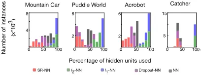
Figure 5: Instance sparsity comparing SR-NN to the regu-larized variants and vanilla NN. The percentage evaluation is designed to disregard units that are never active across all samples in the batch (dead units).
space, depicted in Figure 4(b). The bootstrap estimates, that correspond to the algorithm settings for the learning curves, are plotted in Figure 4(c). We can see that the relative or-dering of the value estimates is maintained with SR-NN and Dropout-NN, which were the two NNs effective for on-policy control, and that their values converge to near the true values (given in Figure 4(d)). The other representations, on the other hand, have very poor estimates. Moreover, these estimates seem to decrease together, suggesting interference is causing overgeneralization to reduce values in other states.
SR-NN `2-NN `1-NN Dropout-NN NN
8.8 111.5 142.5 31.2 54.0
Table 1: Activation overlap in Puddle World. The numbers are the average overlap over all pairs of selected states. For example, SR-NN has an average of 8.8 shared activation over all pais of 5 selected states defined in Figure 4 (a).
sparse on Puddle World, but less so on other domains. The NN representation, which has no regularization, has some instance sparsity, likely due to simply using ReLU activa-tion. Interestingly,`1-NN and`2-NN actually produced less
instance sparsity.
Activation overlap, introduced by French(1991), reflects the amount of shared activation between any two inputs. We consider a variant of activation overlap that measures the number of shared activation between two representations,
φ(x1)andφ(x2), for two samples,x1, andx2:
overlap(φ(x1),φ(x2))
=X
j
1[(φj(x1)>0)∧(φj(x2)>0)].
We measure the activation overlap of the five chosen states, distributed across Puddle World. If the overlap between two representations is zero, the interference would be zero. Up-dating the value function with respect to one state, therefore, would not affect the other state’s value. Table 1 shows the average overlap, and once again, a similar trend emerges where, SR-NN has significantly less overlap (about 8), with Dropout-NN showing the next least overlap (with about 30).
Overall, these results provide some evidence that (a) sparse representations can improve control performance in an in-cremental learning setting, (b) these sparse representations appear to provide locality and (c) this locality reduces interfer-ence and improves accuracy of bootstrap values in Sarsa(0). These results are a first step, and warrant further investi-gation. They do nonetheless motivate that learning sparse representations could be a promising direction for control in reinforcement learning. In the next section, we discuss how we actually obtain such sparse representations (SR-NN).
Distributional Regularizers for Sparsity
In this section, we describe how to use Distributional Regu-larizers to learn sparse representations with neural networks.2 We introduce a Set Distributional Regularizer, which when paired with ReLU activations enables sparse representations to be learned, as we demonstrate in the next section. We first describe how to define Distributional Regularizers on neural networks, and then discuss the extension to a Set Distribu-tional Regularizer, and motivation for doing so.2The idea was originally introduced for neural networks with
Sigmoid activations in an unpublished set of notes (Ng 2011), and as yet has not been systematically explored. When used out-of-the-box, we found important limitations in the learned representations, including from using Sigmoid activations instead of ReLU and from using the KL to a specific distribution. We explore the idea in-depth here, to make it a practical option for learning sparse representations.
The goal of using Distributional Regularizers is to encour-age the distribution of each hidden node—across samples—to match a desired target distribution. In a neural network, we can view the hidden nodes,Y1, . . . , Yd, as random variables,
with randomness due to random inputs. Each of these random variablesYjhas a distributionpβˆj(θ), where the parameters
ˆ
βj(θ)of this distribution are induced by the weightsθof the
neural network:
pβˆj(θ)(y) = Z
s∈S
p(s)p(φj,θ(s) =y)ds.
This provides a distribution over the values for the feature
φj,θ(s), across inputss. A Distributional Regularizer is a KL divergenceKL(pβ||pβˆ
j(θ))that encourages this distribution to match a desired target distributionpβwith parameterβ.
Such a regularizer can be used to encourage sparsity, by se-lecting a target distribution that has high mass or density at zero. Consider a Bernoulli distribution for activations, withYj ∈ {0,1}. Using a Bernoulli target distribution with β = 0.1, givingpβ(Y = 1) = 0.1, encodes a desired
activa-tion of 10%. As another example, for continuous nonnegative
Yj, the target distribution can be set to an exponential
distribu-tionpβ(y) =β
−1exp(
−y/β), which has highest density at zero with expected valueβ. Settingβ = 0.1encourages the average activation to be0.1and increases density ony= 0. The efficacy of this regularizer, however, is tied to the pa-rameterization of the network, which should match the target distribution. For a ReLU activation, for example, which has a range[0,∞), a Bernoulli target distribution is not appropri-ate. Rather, for the range[0,∞), an exponential distribution is more suitable. For a Sigmoid activation, giving values between[0,1], a Bernoulli is reasonably appropriate. Addi-tionally, the parametrization should be able to set activations to zero. The ReLU activation naturally enables zero values (Glorot, Bordes, and Bengio 2011), by pushing activations to negative values. The addition of a Distributional Regularizer simply encourages this natural tendency, and is more likely to provide sparse representations. Activations under Sigmoid and tanh, on the other hand, are more difficult to encourage to zero, because they require highly negative input values or input values exactly equal to 0.5, respectively, to set the hid-den node to zero. For these reasons, we advocate for ReLU for the sparse layer, with an exponential target distribution.
Finally, we modify this regularizer to provide a Set Distri-butional Regularizer, which does not require an exact level of sparsity to be achieved. It can be difficult to choose a precise level of sparsity, making the Distributional Regularizer prone to misspecification. Rather, the actual goal is typically to ob-tainat leastsome level of sparsity, where some nodes can be even more sparse. For this modification, we specify that the distribution should match any of a set of target distributions
Qβ, giving a Set KL: minp∈QβKL(p||pβˆj(θ)). Generally, this Set KL can be hard to evaluate. However, as we show below, it corresponds to a simple clipped KL-divergence for certain choices ofQβ, importantly including for exponential
distributions whereQβ ={pβ˜|β˜≤β}.
Theorem 1(Set KL as a Clipped-KL). Let pη be a
parameterη,B = [η1, η2]be a convex set in the natural
parameter space andQB={pη:η∈B}. Then the Set KL
divergence
SKL(QB||pη) := min
p∈QB
KL(p||pη) (3)
is (a) non-negative (b) convex inηand (c) corresponds to a simple clipped form
SKL(QB||pη) =
KL(pη2||pη) ifη > η2 KL(pη1||pη) ifη < η1
0 else
(4)
Proof. For exponential families, the KL divergence
corre-spond to a Bregman divergence (Banerjee et al. 2005):
KL(pη1||pη) =DF(η||η1)
for a convex potential functionF that depends on the expo-nential family. Hence, we have
SKL(QB||pη) = arg min
˜
η∈BDF(η||η˜)
Ifη∈B, this minimum over Bregman divergences is clearly zero. Ifη < η1andη > η2, we have to consider the
mini-mization. The Bregman divergence is not necessarily convex in the second argument. Instead, we can rely on convexity of the setB. Taking the derivative ofDF(η||η˜)wrtη˜, we get
d
dη˜DF(η||η˜) = d dη˜
F(η)−F(˜η)−(η−η˜) d dη˜F(˜η)
=− d
dη˜F(˜η) + d
dη˜F(˜η)−(η−η˜) d2 dη˜2F(˜η)
=− d
2
dη˜2F(˜η)(η−η˜)
Now becauseFis convex,−d2
d˜η2F(˜η)is always negative. The
derivative, then, is negative whenη < η˜ , indicatingη˜should be increased to decreaseDF(η||η˜). Similarly, whenη > η˜ ,
the derivative is positive, indicatingη˜should be decreased to decreaseDF(η||η˜). This derivative, then, pointsη˜to the
boundaries whenη /∈B, respectively to the boundary points closest toη.
Corollary 1(SKL for Exponential Distributions). Forpβan
exponential distribution, with natural parameterη=−β−1 ,
andB= (0, β], then
SKL(QB||pβˆ) =
(
log ˆβ+βˆ
β−logβ−1 if
ˆ β > β
0 else (5)
We use the SKL in Corollary 1, to encode a sparsity level of at leastβ—rather than exactlyβ—for the last layer in a two-layer neural network with ReLU activations. This regularizer was used to encourage sparse activations for SR-NN in the preceding section. We include pseudocode for optimizing the regularized objective with the SKL, in Algorithm 1 in the Appendix.
6
2
100 50 0
Number of instances
(x*10
3 )
3
1
100 50 0
Mountain Car
6
2
100 50 0
Puddle World
6
2
100 50 0
Acrobot Catcher
Percentage of hidden units used
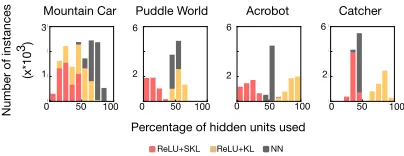
ReLU+SKL ReLU+KL NN
Figure 6: Instance sparsity as evaluated on a batch of test data comparing ReLU+KL and ReLU+SKL to NN. While ReLU+KL can make representations denser than just NN, ReLU+SKL always results in sparser representations.
Evaluation of Distributional Regularizers
In this section, we investigate the efficacy of Distributional Regularizers for obtaining sparsity. There are a variety of possible choices with Distributional Regularizers, including activation function and corresponding target distribution and using a KL versus a Set KL. In this section, we investigate some of these combinations, particularly focusing on the difference in sparsity and performance when using (a) KL versus SKL; (b) Sigmoid (with a Bernoulli target distribution) versus ReLU (with an Exponential target distribution); and (c) previous strategies to obtain sparse representations versus the proposed variant of the Distributional Regularizer.
In the first set of experiments, we compare the instance sparsity of KL to Set KL, with ReLU activations and Expo-nential Distributions (ReLU+KL and ReLU+SKL). Figure 6 shows the instance sparsity for these, and for the NN with-out regularization. Interestingly, ReLU+KL actually reduces sparsity in several domains, because the optimization encour-aging an exact level of sparsity is quite finicky. ReLU+SKL, on the other hand, significantly improves instance sparsity over the NN. This instance sparsity again translates into con-trol performance, where ReLU+KL does noticeably worse than ReLU+SKL across the four domains in Figure 7. Despite the poor instance sparsity, ReLU+KL does actually seem to provide some useful regularity, that does allow some learning across all four domains. This contrasts the previous regular-ization strategies,`2,`1and Dropout, which all failed to learn
on at least one domain, particularly Catcher.
SIG+SKL use all the hidden nodes for all the samples across domains, resulting in no instance sparsity.
Cumulative r
ewar
d per episode
-200
-400
-600
-100
-300
-600
-200
-600
-1000
50
0 100
50 50 100
100
50 500 1000
ReLU+SKL ReLU+SKL
ReLU+SKL
ReLU+SKL ReLU+KL
SIG+KLSIG+SKL
Mountain Car Puddle World
Acrobot Catcher
ReLU+KL
ReLU+KL
ReLU+KL
SIG+SKL
SIG+SKL
SIG+SKL
SIG+KL SIG+KL
SIG+KL
Episode number
Figure 7: Learning curves for Sarsa(0) with different Distri-butional Regularizers.
0.0 0.1 0.0 0.18 0.1 0.25 0.18 0.22
ReLU+SKL ReLU+KL SIG+SKL SIG+KL
Figure 8: Heatmaps of activations with different Distribu-tional Regularizers in Puddle World.
Next, we compare to previously proposed strategies for learning sparse representations with neural networks. These include using`1and`2regularization on the activation
(de-noted by`1R-NN and`2R-NN respectively); k-sparse NNs,
where all but the topkactivations are zeroed (Makhzani and Frey 2013) (k-sparse-NN); and Winner-Take-All NNs that keep the top k% of the activations per node across instances, to promote sparse activations of nodes over time (Makhzani and Frey 2015) (WTA-NN).3
We include learning curves and instance sparsity for these methods, for a ReLU activation, in Figures 9 and 10. Results for the Sigmoid activation are included in the Appendix. Nei-ther WTA-NN nor k-sparse-NN are effective. We found the k-sparse-NN was prone to dead units, and often truncates non-negligible value. Surprisingly,`2R-NN performs
compa-rably to SR-NN in all domains but Catcher, whereas`1R-NN
is effective only during early learning in Mountain Car. From the instance sparsity plots in Catcher, we see that`1R-NN and
3
Both k-sparse-NNs and WTA-NNs were introduced for auto-encoders, though the idea can be applied more generally to NNs. We additionally tested these methods with autoencoders, but perfor-mance was significantly worse.
Cumulative r
ewar
d per episode
-200
-400
100 50
SR-NN
k-sparse-NN
l1R-NN
l2R-NN
WTA-NN
Mountain Car
0
-500
-1000
100 50
Puddle World
SR-NN
k-sparse-NN
l1R-NN
l2R-NN
WTA-NN
-100
-300
100 50
Acrobot
SR-NN
k-sparse-NN
l1R-NN
l2R-NN
WTA-NN 50
0
1000 500
Catcher
SR-NN
k-sparse-NN
l1R-NN l2R-NN
WTA-NN
Episode number
Figure 9: Learning curves for Sarsa(0) comparing SR-NN to previous proposed sparse representations learning strategies.
10
5
10
5
100 50 0 15
10
100 50
0 0 50 100
SR-NN l2R-NN l1R-NN k-sparse-NN WTA-NN
10
5
Number of instances
(x*10
3 )
Percentage of hidden units used
Mountain Car Puddle World Acrobot Catcher
100 50 0
Figure 10: Instance sparsity comparing SR-NN to previous proposed sparse representations learning strategies.
`2R-NN produce highly sparse (2%-3% instance sparsity),
potentially explaining its poor performance. While similar in-stance sparsity was effective in Puddle World, this is unlikely to be true in general. This was with considerable parameter optimization for the regularization parameter.
Conclusion
In this work, we investigate using and learning sparse repre-sentations with neural networks for control in reinforcement learning. We show that sparse representations can signifi-cantly improve control performance when used in an incre-mental learning setting, and provide some evidence that this is because the locality of the representation reduces catas-trophic interference which would otherwise overwrite boot-strap values. We formalize Distributional Regularizers, with a practically important extension to a Set KL, for learning a Sparse Representation Neural Network (SR-NN). We provide an empirical investigation into the sparsity properties and con-trol performance under different Distributional Regularizers, as well as compared to other algorithms to obtain sparse rep-resentations with neural networks. We conclude that SR-NN performs consistently well across domains, with the next best method—which only fails in one domain—being a simple methods that uses an`2regularizer on activations.
inter-ference. Interference is typically considered for sequential multi-task learning, where previous functions are forgotten by training on a new task. Interference could occur even in a single-task setting, if an agent remains in a particular area of the space for a long time. In reinforcement learning, however, this problem is magnified by the fact that the agent uses its own estimates as targets. If estimates change incorrectly due to interference, there could be a cascading effect. This work provides some first empirical steps, in a carefully controlled set of experiments, to identify that this could be an issue, and that sparse representations could be a promising direction to alleviate the problem. We hope for this work to spur fur-ther empirical investigation into how widespread this issue is, and further algorithmic development into learning sparse representations for reinforcement learning.
References
Ahmad, S., and Hawkins, J. 2015. Properties of Sparse Distributed Representations and their Application to Hierarchical Temporal Memory.
Arpit, D.; Zhou, Y.; Ngo, H.; and Govindaraju, V. 2015. Why
regu-larized auto-encoders learn sparse representation? InInternational
Conference on Machine Learning.
Banerjee, A.; Merugu, S.; Dhillon, I. S.; and Ghosh, J. 2005.
Clus-tering with bregman divergences. Journal of Machine Learning
Research6(Oct):1705–1749.
Banino, A.; Barry, C.; Uria, B.; Blundell, C.; Lillicrap, T.; Mirowski, P.; Pritzel, A.; Chadwick, M. J.; Degris, T.; Modayil, J.; et al. 2018. Vector-based navigation using grid-like representations in artificial
agents.Nature.
Bengio, Y.; Courville, A.; and Vincent, P. 2013. Representation
learning: A review and new perspectives. IEEE Transactions on
Pattern Analysis and Machine Intelligence.
Bengio, Y. 2009. Learning deep architectures for AI.Foundations
and Trends in Machine Learning.
Cover, T. M. 1965. Geometrical and Statistical Properties of Sys-tems of Linear Inequalities with Applications in Pattern Recognition.
IEEE Trans. Electronic Computers.
F¨oldi´ak, P. 1990. Forming sparse representations by local
anti-Hebbian learning.Biological Cybernetics.
French, R. M. 1991. Using semi-distributed representations to overcome catastrophic forgetting in connectionist networks. In
Annual Cognitive Science Society Conference.
Glorot, X.; Bordes, A.; and Bengio, Y. 2011. Deep sparse
rec-tifier neural networks. InInternational Conference on Artificial
Intelligence and Statistics.
Goodfellow, I.; Lee, H.; Le, Q. V.; Saxe, A.; and Ng, A. Y. 2009.
Measuring invariances in deep networks. InAdvances in Neural
Information Processing Systems.
Kanerva, P. 1988.Sparse Distributed Memory. MIT Press.
Le, L.; Kumaraswamy, R.; and White, M. 2017. Learning
sparse representations in reinforcement learning with sparse coding.
arXiv:1707.08316.
Lee, H.; Ekanadham, C.; information, A. N. A. i. n.; and 2008. 2008.
Sparse deep belief net model for visual area V2. InAdvances in
Neural Information Processing Systems.
Lemme, A.; Reinhart, R. F.; and Steil, J. J. 2012. Online learning and generalization of parts-based image representations by non-negative
sparse autoencoders.Neural Networks.
Mairal, J.; Bach, F.; Ponce, J.; Sapiro, G.; and Zisserman, A. 2009.
Supervised dictionary learning. InAdvances in Neural Information
Processing Systems.
Mairal, J.; Bach, F.; Ponce, J.; and Sapiro, G. 2010. Online learning
for matrix factorization and sparse coding. Journal of Machine
Learning Research.
Makhzani, A., and Frey, B. 2013. k-sparse autoencoders. arXiv
preprint arXiv:1312.5663.
Makhzani, A., and Frey, B. 2015. Winner-take-all autoencoders. In
Adv. in Neural Information Processing Systems.
McCloskey, M., and Cohen, N. J. 1989. Catastrophic Interfer-ence in Connectionist Networks: The Sequential Learning Problem.
Psychology of Learning and Motivation.
McCulloch, W. S., and Pitts, W. 1943. A logical calculus of the
ideas immanent in nervous activity.The Bulletin of Mathematical
Biophysics.
Ng, A. 2011. Sparse autoencoder. CS294A Lecture notes.
Olshausen, B. A., and Field, D. J. 1997. Sparse coding with
an overcomplete basis set: A strategy employed by V1? Vision
Research.
Olshausen, B. A. 2002. Sparse Codes and Spikes. InProbabilistic
Models of the Brain.
Quian Quiroga, R., and Kreiman, G. 2010. Measuring sparseness in the brain: Comment on bowers (2009).
Ranzato, M.; Poultney, C. S.; Chopra, S.; and LeCun, Y. 2006. Efficient Learning of Sparse Representations with an Energy-Based
Model. InAdv. in Neural Info. Process. Sys.
Ranzato, M.; Boureau, Y.-L.; and LeCun, Y. 2007. Sparse
Fea-ture Learning for Deep Belief Networks. InAdvances in Neural
Information Processing Systems.
Ratitch, B., and Precup, D. 2004. Sparse distributed memories for
on-line value-based reinforcement learning. InMachine Learning:
ECML PKDD.
Riedmiller, M. 2005. Neural fitted Q iteration–first experiences with
a data efficient neural reinforcement learning method. InEuropean
Conference on Machine Learning.
Rifai, S.; Vincent, P.; Muller, X.; Glorot, X.; and Bengio, Y. 2011. Contractive auto-encoders: Explicit invariance during feature
extrac-tion. InInter. Conf. on Machine Learning.
Srivastava, N.; Hinton, G.; Krizhevsky, A.; Sutskever, I.; and Salakhutdinov, R. 2014. Dropout: a simple way to prevent
neu-ral networks from overfitting. The Journal of Machine Learning
Research15(1):1929–1958.
Sutton, R. S., and Barto, A. G. 1998.Reinforcement learning: An
introduction. MIT press Cambridge.
Sutton, R. S. 1996. Generalization in reinforcement learning:
Successful examples using sparse coarse coding. InAdvances in
Neural Information Processing Systems.
Teh, Y. W.; Welling, M.; Osindero, S.; and Hinton, G. E. 2003. Energy-Based Models for Sparse Overcomplete Representations.
Journal of Machine Learning Research.
Triesch, J. 2005. A Gradient Rule for the Plasticity of a Neuron’s
Intrinsic Excitability. InICANN.
White, M. 2017. Unifying Task Specification in Reinforcement