Training Temporal Word Embeddings with a Compass

The Thirty-Third AAAI Conference on Artificial Intelligence (AAAI-19)

Training Temporal Word Embeddings with a Compass

Valerio Di Carlo,

Federico Bianchi,

Matteo Palmonari

[email protected], [email protected], [email protected]

Abstract

Temporal word embeddings have been proposed to support the analysis of word meaning shifts during time and to study the evolution of languages. Different approaches have been proposed to generate vector representations of words that embed their meaning during a specific time interval. How-ever, the training process used in these approaches is com-plex, may be inefficient or it may require large text corpora. As a consequence, these approaches may be difficult to ap-ply in resource-scarce domains or by scientists with limited in-depth knowledge of embedding models. In this paper, we propose a new heuristic to train temporal word embeddings based on the Word2vec model. The heuristic consists in us-ing atemporal vectors as a reference, i.e., as acompass, when training the representations specific to a given time interval. The use of thecompass simplifies the training process and makes it more efficient. Experiments conducted using state-of-the-art datasets and methodologies suggest that our ap-proach outperforms or equals comparable apap-proaches while being more robust in terms of the required corpus size.

Introduction

Language is constantly evolving, reflecting the continuous changes in the world and the needs of the speakers. While new words are introduced to refer to new concepts and ex-periences (e.g., Internet, hashtag, microaggression), some words are subject to semantic shifts, i.e., their meanings change over time (Basile et al. 2016). For example, in the English language, the word gay originally meant joyful, happy; only during the20th century the word began to be used in association with sexual orientation (Kulkarni et al. 2015).

Finding methods to represent and analyze word evolution over time is a key task to understand the dynamics of hu-man language, revealing statistical laws of sehu-mantic evolu-tion (Hamilton, Leskovec, and Jurafsky 2016). In addievolu-tion, time-dependent word representations may be useful when natural language processing algorithms that use these repre-sentations, e.g., an entity linking algorithm (Yamada et al. 2017), are applied to texts written in a specific time period.

Distributional semanticsadvocates a “usage-based” per-spective on word meaning representation: this approach is

Copyright c2019, Association for the Advancement of Artificial Intelligence (www.aaai.org). All rights reserved.

based on thedistributional hypothesis (Firth 1957), which states that the meaning of a word can be defined by the word’scontext.

Word embedding models based on this hypothesis have received great attention over the last few years, driven by the success of the neural network-based model Word2vec (Mikolov et al. 2013a). These models represent word mean-ings as vectors, i.e.,word embeddings. Most state-of-the-art approaches, including Word2vec, are formulated as static models. Since they assume that the meaning of each word is fixed in time, they do not account for the semantic shifts of words. Thus, recent approaches have tried to capture the dynamics of language (Hamilton, Leskovec, and Ju-rafsky 2016; Bamler and Mandt 2018; Szymanski 2017; Yao et al. 2018; Rudolph and Blei 2018).

A Temporal Word Embedding Model (TWEM) is a model that learnstemporal word embeddings, i.e., vectors that rep-resent the meaning of words during a specific temporal in-terval. For example, a TWEM is expected to associate dif-ferent vectors to the wordgayat different times: its vector in1900is expected to be more similar to the vector ofjoyful than its vector in 2005. By building a sequence of tempo-ral embeddings of a word over consecutive time intervals, one can track the semantic shift occurred in the word usage. Moreover, temporal word embeddings make it possible to find distinct words that share a similar meaning in different periods of time, e.g., by retrieving temporal embeddings that occupy similar regions in the vector spaces that correspond to distinct time periods.

have to be aligned.

Most of the proposed TWEMs align multiple vector spaces by enforcing word embeddings in different time periods to be similar (Kulkarni et al. 2015; Rudolph and Blei 2018). This method is based on the assumption that the majority of the words do not change their meaning over time. This approach is well motivated but may lead, for some words, to excessively smoothen differences be-tween meanings that have shifted along time. A remark-able limitation of current TWEMs is related to the assump-tions they make on the size of the corpus needed for train-ing: while some methods like (Szymanski 2017; Hamilton, Leskovec, and Jurafsky 2016) require a huge amount of training data, which may be difficult to acquire in several application domains, other methods like (Yao et al. 2018; Rudolph and Blei 2018) may not scale well when trained with big datasets.

In this work we propose a new heuristic to train temporal word embeddings that has two main objectives: 1) to be sim-ple enough to be executed in ascalable and efficientmanner, thus easing the adoption of temporal word embeddings by a large community of scientists, and 2) to produce models that achievegood performancewhen trained with both small and big datasets.

The proposed heuristic exploits the often overlooked dual representation of words that is learned in the two Word2vec architectures: Skip-gram and Continuous bag-of-words (CBOW) (Mikolov et al. 2013a). Given a target word, Skip-gram tries to predict its contexts, i.e., the words that oc-cur nearby the target word (where “nearby” is defined using a window of fixed size); given a context, CBOW tries to pre-dict the target word appearing in that context. In both archi-tectures, each word is represented by atarget embeddingand acontext embedding. During training, the target embedding of each word is placed nearby the context embeddings of the words that usually appear inside its context. Both kinds of vectors can be used to represent the word meanings (Ju-rafsky and Martin 2000).

The heuristic consists in keeping one kind of embeddings frozen across time, e.g., the target embeddings, and using a specific temporal slice to update the other kind of embed-dings, e.g., the context embeddings. The embedding of a word updated with a slice corresponds to its temporal word embedding relative to the time associated with this slice. The frozen embeddings act as an atemporal compass and makes sure that the temporal embeddings are already gener-ated during the training inside a shared coordinate system. In reference to the analogy of the map drawing (Smith et al. 2017), our method draws maps according to a compass, i.e., the reference coordinate system defined by the atempo-ral embeddings.

In a thorough experimental evaluation conducted using temporal analogies and held-out tests, we show that our approach outperforms or equals comparable state-of-the-art models in all the experimental settings, despite its efficiency, simplicity and increased robustness against the size of the training data. The simplicity of the training method and the interpretability of the model (inherited from Word2vec) may foster the application of temporal word embeddings in

stud-ies conducted in related research fields, similarly to what happened with Word2vec which was used, e.g., to study bi-ases in language models (Caliskan, Bryson, and Narayanan 2017).

The paper is organized as follows: in Section 2 we sum-marize the most recent approaches on temporal word em-beddings. In Section 3 we present our model while in Sec-tion 4 we present experiments with state-of-the-art datasets. Section 5 ends the paper with conclusions and future work.

Related Work

Different researchers have investigated the use of word embeddings to analyze semantic changes of words over time (Hamilton, Leskovec, and Jurafsky 2016; Kulkarni et al. 2015). We identify two main categories of approaches based on the strategy applied to align temporal word em-beddings associated with different time periods.

Pairwise alignment-based approaches align pairs of vec-tor spaces to a unique coordinate system: Kim et al. and Tredici, Nissim, and Zaninello align consecutive temporal vectors through neural network initialization; other authors apply various linear transformations after training that min-imize the distance between the pairs of vectors associated with each word in two vector spaces (Kulkarni et al. 2015; Hamilton, Leskovec, and Jurafsky 2016; Szymanski 2017; Zhang et al. 2016).

Joint alignment-based approaches train all the temporal vectors concurrently, enforcing them inside a unique coor-dinate system: Bamman, Dyer, and Smith extend Skip-gram Word2vec tying all the temporal embeddings of a word to a common global vector (they originally apply this method to detect geographical language variations); other models im-pose constraints on consecutive vectors in the PPMI ma-trix factorization process (Yao et al. 2018) or when train-ing probabilistic models to enforce the “smoothness” of the vectors’ trajectory along time (Bamler and Mandt 2018; Rudolph and Blei 2018). This strategy leads to better em-beddings when smaller corpora are used for training but is less efficient then pairwise alignment.

Despite the differences, both alignment strategies try to enforce the vector similarity among different temporal em-beddings associated with a same word. While this alignment principle is well motivated from a theoretical and practical point of view, enforcing the vector similarity of one word across time may lead to excessively smooth the differences between its representations in different time periods. Find-ing a good trade-off betweendynamismandstaticnessseems an important feature of a TWEM. Finally, very few models proposed in the literature do not require explicit pairwise or joint alignment of the vectors, and they all rely on co-occurrence matrix or high-dimensional vectors (Gulordava and Baroni 2011; Basile et al. 2016).

Dt1 _Dti _Dtj _DtN

Ct1 _Cti _Ctj _CtN

Atemporal compass D

C U

U U U U

Initialization Training

1

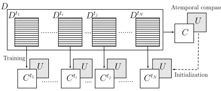
Figure 1: The TWEC model. The temporal context embed-dingsCt_{are independently trained over each temporal slice,}

with frozen pre-trained atemporal target embeddingsU.

align different temporal representations using a shared co-ordinate system instead of enforcing (pairwise or joint) vec-tor similarity in the alignment process; (ii) to rely on neural networks and low-dimensional word embeddings; (iii) to be easy to implement on top of the well-known Word2vec and highly efficient to train.

Temporal Word Embeddings with a Compass

Our approach is based on the same assumption used in previous work, that is, the majority of words do not change their meaning over time (Kulkarni et al. 2015). From this as-sumption, we derive a second one: we assume that a shifted word, i.e., a word whose meaning has shifted across time, appears in the contexts of words whose meaning changes slightly. However, differently from the latter assumption, our assumption is particularly true for shifted words. For exam-ple, the wordclintonappears during some temporal periods in the contexts of words that are related to his position as president of the USA (e.g.,president,administration); con-versely, the meanings of these words have not changed. The above assumption allows us to heuristically consider the tar-get embeddings as static, i.e., to freeze them during training, while allowing the context embeddings to change based on co-occurrence frequencies that are specific to a given tem-poral interval. Thus, our training method returns the context embeddings as temporal word embeddings.

Finally, we observe that our compass method can be ap-plied also in the opposite way, i.e., by freezing the con-text embeddings and moving the target embeddings, which are eventually returned as temporal embeddings. However, a thorough comparison between these two specular compass-based training strategies is out of the scope of this paper.

TWEC can be implemented on top of the two Word2vec models, Skip-gram and CBOW.

Here we present the details of our model using CBOW as underlying Word2vec model, since we empirically found that it produces temporal models that show better perfor-mance than Skip-gram with small datasets. We leave to the reader the interpretation of our model when Skip-gram is used.

In the CBOW model, context embeddings~cjare encoded

in theinput weight matrix Cof the neural network, while

target embeddings~uk are encoded inside theoutput weight

matrixU(vice-versa in the Skip-gram model). Let us con-sider a diachronic corpusDdivided inntemporal slicesDti_,

with1≤i≤n. The training process of TWEC is divided in two phases, which are schematically depicted in Figure 1.

(i) First, we construct twoatemporalmatricesCandUby applying the original CBOW model on the whole diachronic corpusD, ignoring the time slicing;CandUrepresents the set ofatemporal context embeddingsandatemporal target embeddings, respectively. (ii) Second, for each time slice

Dti_{, we construct a temporal context embedding matrixC}ti

as follows. We initialize the output weight matrix of the neu-ral network with the previously trained target embeddings from the matrixU. We run the CBOW algorithm using the temporal slice Dti_{. During this training process, the target}

embeddings of the output matrixUare not modified, while we update the context embeddings in the input matrixCti_.

After applying this process on all the time slicesDti_{, each}

input matrixCti _{will represent our temporal word}

embed-dings at the timeti. Here below we further explain the key

phase in our model, that is, the update of the input matrix for each slice, and the interpretation of the update function in our temporal model.

Given a temporal sliceDt, the second phase of the train-ing process can be formalized for a strain-ingle traintrain-ing sample hwk, γ(wk)i ∈Dtas the following optimization problem:

max

Ct logP(wk|γ(wk)) =σ(~uk·~c

t

γ(wk)) (1)

whereγ(wk) =hwj1,· · ·, wjMirepresents theM words in

the context ofwk which appear inDt(M₂ is the size of the

context window),~uk ∈Uis the atemporal target embedding

of the wordwk, and

~c_γt_(w k)=

1

M(~c

t

j1+· · ·+~c

t jM)

T ₍₂₎

is the mean of the temporal context embeddings~ct jm of the

contextual wordswjm. The softmax functionσis calculated

using Negative Sampling (Mikolov et al. 2013b). Please note that Ct is the only weight matrix to be optimized in this phase (Uis constant), which is the main difference from the classic CBOW. The training process maximizes the proba-bility that given the context of a wordwkin a particular

tem-poral slicet, we can predict that word using the atemporal target matrixU. Intuitively, it moves the temporal context embedding~ct

jm closer to the atemporal target embeddings ~

ukof the words that usually have the wordwjmin their

con-texts during the timet. The resulting temporal context em-beddings can be used as temporal word emem-beddings: they will be already aligned, thanks to the shared atemporal tar-get embeddings used as a compass during the independent trainings.

Data

Words

Span

Slices

NAC-S

50

M

1990

-

2016

27

NAC-L

668

M

1987

-

2007

21

MLPC

6

.

5

M

2007

-

2015

9

Test

Analogies

Span

Categories

T1

11

,

028

1990

-

2016

25

T2

4

,

200

1987

-

2007

10

Table 1: Details of NAC-S, NAC-L, MLPC, T1 and T2.

CBOW over the entire corpusD, plus the task of comput-ingnCBOW models over all the time slices.

We observe that, differently from those approaches that enforce similarity between consecutive word embeddings (e.g., Rudolph and Blei), TWEC does not apply any time-specific assumption. In the next section, we show that this feature does not affect the quality of the temporal word em-beddings generated using TWEC. Otherwise, this feature makes TWEC’s training process more general and applica-ble to corpora sliced using different criteria, e.g., a news cor-pus split by location, publisher, or topic, to study differences in meaning that depend on factors other than time.

Experiments

In this section, we discuss the experimental evaluation of TWEC. We compare TWEC with static models and with the state-of-the-art temporal models that have shown better per-formance according to the literature. We use the two main methodologies proposed to evaluate temporal embeddings so far: temporal analogical reasoning (Yao et al. 2018) and held-out tests (Rudolph and Blei 2018). Our experiments can be easily replicated using the source code available online1_.

Experiments on Temporal Analogies

DatasetsWe use two datasets with different sizes to test the effects of the corpus size on the models’ performances. The small dataset (Yao et al. 2018) is freely available online2. We will refer to this dataset as News Article Corpus Small (NAC-S). Thebig datasetis the New York Times Annotated Corpus3 _{(Sandhaus 2008) employed by Szymanski; Zhang} et al. to test their TWEMs. We will refer to this dataset as News Article Corpus Large (NAC-L). Both datasets are di-vided into yearly time slices.

We chose two test sets from those already available: Test-set1 (T1) introduced by Yao et al. and Testset2 (T2) intro-duced by Szymanski. They are both composed of tempo-ral word analogies based on publicly recorded knowledge, partitioned in categories (e.g.,President of the USA, Super Bowl Champions). The main characteristics of datasets and test sets are summarized in Table 1.

MethodologyTo test the models trained on NAC-S we used the T1, while to test the models trained on NAC-L we used the T2. This allows us to replicate the settings of the work

1_{https://github.com/valedica/twec} 2

https://sites.google.com/site/zijunyaorutgers/publications

3

https://catalog.ldc.upenn.edu/ldc2008t19

of Yao et al. and Szymanski respectively. We quantitative evaluate the performance of a TWEM in the task of solving temporal word analogies (TWAs) (Szymanski 2017). The task of solving a temporal word analogy, given in the form

w1 : t1 = x : t2, is to find the word w2 that is the most semantically similar word int2to the input wordw1int1, wheret1andt2are temporal intervals. Because semantically similar words result in distributional similar ones, it follows that two words involved in a TWA will occupy a similar po-sition in the vector space at different points in time. Then, solving the TWA w1 : t1 = x : t2consists in finding the nearest vector at timet2to the input vector of the wordw1 at timet1. For example, we expect that the vector of the word clintonin1997will be similar to the vector of the word rea-ganin1987.

Given an analogyw1:t1=x:t2, we definetime depth

δtas the distance between the temporal intervals involved in

the analogy:δt=|t1−t2|. Analogies can be divided in two subsets: the setStaticofstatic analogies, which involve a pair of the same words (obama : 2009 = obama : 2010), and the set Dynamic (Dyn.)of dynamic analogies, that are not static. We refer to the complete set of analogies as

All. Given a TWEM an a set of TWAs, the evaluation on the given answers is done with the use of two standard metrics, the Mean Reciprocal Rank (MRR) and

AlgorithmsWe tested different models to compare the re-sults of TWEC with the ones provided by the state-of-the-art: two models that apply pairwise alignment, two mod-els that apply joint alignment and a baseline static model. Where not stated differently, we implemented them with CBOW and Negative Sampling extending the gensim li-brary. The compare TWEC with the following models:

• LinearTrans-Word2vec(TW2V) (Szymanski 2017). • OrthoTrans-Word2vec(OW2V) (Hamilton, Leskovec, and

Jurafsky 2016).

• Dynamic-Word2vec(DW2V) (Yao et al. 2018). The orig-inal model was not available for replication at the time of the experiments. However, they provide the dataset and the test set of their evaluation settings (the same employed in our experiments) and published their results using our same metrics. Thus, the model can be compared to our using the same parameters.

• Geo-Word2vec (GW2V) (Bamman, Dyer, and Smith 2014). We use the implementation provided by the au-thors.

• Static-Word2vec(SW2V): a baseline adopted by Yao et al. and Szymanski. The embeddings are learned over all the diachronic corpus, ignoring the temporal slicing.

We also tested the model defined by Rudolph and Blei and we obtained results close to the baseline SW2V, confirming what reported by Barranco, Santos, and Hossain; Thus, we do not report the results for their model on the analogy task.

Model Set MRR MP1 MP3 MP5 MP10

SW2V Static 1 1 1 1 1

Dyn. 0.148 0.000 0.263 0.351 0.437

All 0.375 0.266 0.459 0.524 0.587

TW2V Static 0.245 0.193 0.280 0.313 0.366 Dyn. 0.106 0.069 0.123 0.156 0.205

All 0.143 0.102 0.165 0.198 0.248

OW2V Static 0.265 0.202 0.299 0.348 0.415 Dyn. 0.087 0.058 0.099 0.124 0.160

All 0.135 0.096 0.153 0.183 0.228

DW2V Sta − − − − −

Dyn. − − − − −

All 0.422 0.331 0.485 0.549 0.619

GW2V Static 0.857 0.819 0.888 0.909 0.931 Dyn. 0.071 0.005 0.092 0.159 0.225

All 0.280 0.222 0.305 0.359 0.435

TWEC Static 0.720 0.668 0.763 0.787 0.813 Dyn. 0.394 0.308 0.451 0.508 0.571

All 0.481 0.404 0.534 0.582 0.636

Table 2: MRR and MP for the subsets of static and dynamic analogies of T1. We use MPK in place of MP@K. DW2V results are taken from the original paper (Yao et al. 2018).

and a small vocabulary of21k words with at least200 oc-currences over the entire corpus. Table 2 summarizes the re-sults.

We can see that TWEC outperforms the other models with respect to all the employed metrics. In particular, it performs better than DW2V, giving 7% more correct an-swers. DW2V confirms its superiority with respect to the pairwise alignment methods, as in Yao et al.. Unfortunately, due to the lack of the answers set and the embeddings, we can not know how well it performs over static and dynamic analogies separately. TW2V and OW2V scored below the static baseline (as in Yao et al.), particularly on analogies with small time depth (Figure 2). In this setting, the pair-wise alignment approach leads to huge disadvantages due to data sparsity: the partitioning of the corpus produces tiny slices (around3.5k news articles) that are not sufficient to properly train a neural network; the poor quality of the em-beddings affects the subsequent pairwise alignment. As ex-pected, SW2V’s accuracy on analogies drops sharply as time depth increases (Figure 2). On the contrary, TWEC, TW2V and OW2V maintain almost steady performances over dif-ferent time depths. GW2V does not answer correctly almost any dynamic analogies. We conclude that GW2V alignment is not capable of capturing the semantic dynamism of words across time for the analogy task. For this reason, we do not employ it in our second setting.

The comparison of the models’ performances across the 25categories of analogies contained in T1 reveals new infor-mation: TW2V and OW2V’s correct answers cover mainly 4categories, likePresident of the USAandPresident of the Russian Federation; TWEC scores better over all the cate-gories. Some categories are more difficult than others: even TWEC scores nearly0% in many categories, likeOscar Best Actor and ActressandPrime Minister of India. This discrep-ancy may be due to various reasons. First of all, some cate-gories of words are more frequent than others in the corpus,

Figure 2: Accuracy (MP@1) as function of time depthδtin

T1. Given an analogyw1 : w2 =t1 : t2, the time depth is plotted asδt=|t1−t2|.

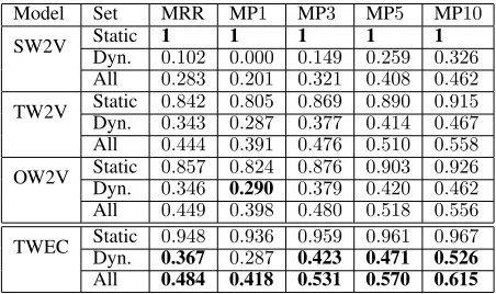
Model Set MRR MP1 MP3 MP5 MP10

SW2V Static 1 1 1 1 1

Dyn. 0.102 0.000 0.149 0.259 0.326

All 0.283 0.201 0.321 0.408 0.462

TW2V Static 0.842 0.805 0.869 0.890 0.915 Dyn. 0.343 0.287 0.377 0.414 0.467

All 0.444 0.391 0.476 0.510 0.558

OW2V Static 0.857 0.824 0.876 0.903 0.926 Dyn. 0.346 0.290 0.379 0.420 0.462

All 0.449 0.398 0.480 0.518 0.556

TWEC Static 0.948 0.936 0.959 0.961 0.967 Dyn. 0.367 0.287 0.423 0.471 0.526

All 0.484 0.418 0.531 0.570 0.615

Table 3: MRR and MP for the subsets of static and dynamic analogies of T2. We use MPK in place of MP@K.

so their embeddings are better trained. For example,obama occurs20,088times in NAC-S, whereasdicaprioonly260. As noted by Yao et al., in the case of some categories of words, like presidents and mayors, we are heavily assisted by the fact that they commonly appear in the context of a title (e.g.President Obama,Mayor de Blasio). For example in TWEC,obamaduring its presidency is always the nearest context embedding to the wordpresident. Lastly, as noted by Szymanski, some roles involved in the analogies only in-fluence a small part of an entity’s overall news coverage. We show that this is reflected in the vector space: as we can see in Figure 4, presidents’ embeddings almost cross each other during their presidency, because they share a lot of contexts; on the other hand, football teams’ embeddings remain dis-tant.

Figure 3: Accuracy (MP@1) as function of time depthδtin

T2. Given an analogyw1 :w2 = t1 : t2, the time depth is plotted asδt=|t1−t2|.

Category SW2V TW2V OW2V TWEC

President of the USA 0.4000 0.9905 0.9905 0.8833 Secret. of State (USA) 0.1190 0.3000 0.3619 0.3405

Mayor of NYC 0.2476 0.9643 0.9524 0.9405

Gover. of New York 0.4476 0.9333 0.9381 0.9786 Super Bowl Champ. 0.0571 0.2024 0.2524 0.1452

NFL MVP 0.0190 0.0143 0.0143 0.0190

Oscar Best Actress 0.0095 0.0119 0.0071 0.0119 WTA Top Player 0.1619 0.2071 0.1548 0.2857 Goldman Sachs CEO 0.1762 0.0143 0.0238 0.1190 UK Prime Minister 0.3762 0.2762 0.2857 0.4595

Table 4: Accuracy (MP@1) for the subsets of the analogy categories in T2. The best scores are highlighted.

TWEC still outperforms all the other models with respect to all the metrics, although its advantage is less than in the previous setting. Generally, we can say that TWEC assigns lower ranks to correct answer words comparing to TW2V and OW2V; however it assigns the first position to them as frequently as the competing models. Table 3 shows that the advantage of TWEC is limited to the static analogies. TW2V and OW2V score much better results than in the previous setting. This is due to the increased size of the input dataset which allows the training process to work well on individual slices of the corpus.

In Figure 3 we can see how the three temporal models behave similarly with respect to the time depth of the analo-gies.

The comparison of the models’ performances across the 10categories of analogies contained in T2 reveals more dif-ferences between them. The results in terms of MP@1 are summarized in Table 4. TW2V and OW2V significantly out-perform TWEC in two categories:President of the USAand Super Bowl Champions. In both cases, this is due to the ma-jor accuracy on dynamic analogies; most of the time, TWEC is wrong because it gives static answers to dynamic analo-gies. TWEC significantly outperforms the other models in two categories:WTA Top-ranked PlayerandPrime Minister of UK. However in this case, TWEC outperforms them both on dynamic and static analogies.

Figure 4: 2-dimensional PCA projection of the temporal em-beddings of pairs of words from clinton, bush and49ers, patriots. The dot points highlight the temporal embeddings during their presidency or their winning years.

Experiments on Held-Out Data

In this section we show the performance of the TWEC on an held-out task. We perform this test in two different ways. We tried to replicate the likelihood based experiments in Rudolph and Blei and to further give confirmation about the performance of our model we also test the posterior probabilities using the framework described in Taddy. Given a model, Rudolph and Blei assign a Bernoulli probability to the observed words in each held-out position: this metric is straightforward because it corresponds to the probability that appears in Equation 1. However, at the implementation level, this metric is highly affected by the magnitude of the vectors because is based on the dot product of the vectors~uk

and~cγ(wk). In particular, Rudolph and Blei applied L2

reg-ularization on the embeddings, which prioritize vectors with small magnitude.

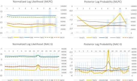
pre-Figure 5:Lt

VandPVt for each test sliceTtand modelV. Blue bars represent the number of words in each slice.

processing script of Rudolph and Blei to prepare the NAC-S dataset for training and testing (|V|= 21,000).

Methodology A We measure the held-out likelihood fol-lowing a methodology similar to Rudolph and Blei. Given a TWEM V = {Vt∈1···T} = {hCt∈1···T,Ut∈1···Ti}, we

calculate the log-likelihood for the temporal testing slice Tt_=hw

1,· · ·, wNias:

logPVt(T

t

) =

N

X

n=1

logPVt(wn|γ(wn)) (3)

where the probability logPVt(wn|γ(wn)) is calculated

based on Equation 1 using Negative Sampling and the vec-tors ofCt_andUt_{. As Rudolph and Blei, we equally}

bal-ance the contribution of the positive and negative samples. For each modelV, we report the value of the normalized log likelihoodLt_:

Lt

V=

1

N logPV(T

t_{) (4)}

and its arithmetic meanLVover all the slices.

Methodology BWe adapt the methodology of Taddy to the evaluation of TWEM. We calculate the posterior probabil-ity of assessing a temporal testing slice Tt _{to the correct}

temporal class labelt. In our setting, this corresponds to the probability that a modelVpredicts the year of thet-th slice given an held-out text from the same slice. We apply Bayes rules to calculate this probability:

PVt(t|T

t_{) =} PVt(T

t_)P(t)

PT

k=1PVk(T

t_)P(k) (5)

A good temporal modelV ={Vt∈1···T}will assign an high

likelihood to the sliceTt_{using the vectors ofV}

tand a

rela-tively low likelihood using the vectors ofVk6=t. We assume

that the prior probability on class labeltis the same for each class,P(t) = 1/T. For implementation reason, we redefine the posterior likelihood as:

Pt

V=PVt(t|T

t_{) =} 1

S

S

X

s=1

PVt(z

t s)P(t)

PT

k=1PVk(z

t s)P(k)

(6)

wherezsis thes-th sentence inTtandPVt(zs)is calculated

based on Equation 3. Please note that this metric is not af-fected by the magnitude of the vectors because is based on a ratio of probabilities. For each modelV, we report the value of the posterior log probabilityPt

V and its arithmetic mean

PVover all the slices.

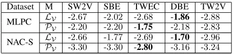
Dataset M SW2V SBE TWEC DBE TW2V

MLPC LV -2.67 -2.02 -2.68 -1.86 -2.88 PV -2.20 -2.20 -1.75 -2.18 -2.83

NAC-S L_PV -2.66 -1.77 -2.69 -1.70 -2.96

V -3.30 -3.30 -2.80 -3.16 -3.24

Table 5: The arithmetic mean of the log likelihoodLV and

of the posterior log probabilityPVfor each modelV. Based

on the standard error on the validation set, all the reported results are significant.

rate η = 0.0025, window of size 1, embeddings of size 50and10iterations (5 static and5dynamic for TWEC,1 static and9dynamic for DBE as suggested by Rudolph and Blei). Following Rudolph and Blei, before the second phase of the training process of TWEC, we initialize the temporal models with both the weight matricesCandUof the static model: we note that this improves held-out performances but it negatively affects the analogy tests. We limit our study to small datasets and small embeddings due to the computa-tional cost: DBE takes almost6hours to train on NAC-S on a16-core CPU setting. DBE and SBE are implemented by the authors usingtensorflow, while all the other models are implemented ingensim: to evaluate them, we convert them togensimmodels, extracting the matricesUt_andC.

Results

Table 5 shows the mean results of the two metrics for each model. In both settings, TWEC obtain a likelihood almost equal to SW2V but a much better posterior probability than the baseline. This is remarkable considering that TWEC op-timizes the scoring function only on one weight matrixCt_,

keeping the matrixUt_{frozen. Comparing to TW2V, TWEC}

has a better likelihood and its posterior probability is more stable across slices (Figure 5). The likelihood scores of DBE and SBE are highly influenced by the different magnitude of their vectors: we can quantify the contribution of the applied L2 regularization comparing the two static baseline SBE and SW2V. Differently from TWEC, DBE slightly improves the likelihood with respect to its baseline. However, regarding the posterior probability, TWEC outperforms DBE. Our ex-periments suggest an inverse correlation between the capa-bility of generalization and the capacapa-bility of extracting dis-criminative features from small diachronic datasets. Finally, experimental results show that TWEC captures discrimina-tive features from temporal slices without losing generaliza-tion power.

Conclusions and Future Work

In this paper, we have presented a novel approach to train temporal word embeddings using atemporal embeddings as a compass. The approach is scalable and effective. While the idea of using an atemporal compass to align slices implicitly surfaced in previous work, we encode this principle into a training method based on neural networks, which makes it simpler and efficient.

Results of a comparative experimental evaluation based on datasets and methodologies used in previous work

sug-gest that, despite its simplicity and efficiency, our approach builds models that are of equal or better quality than the ones generated with comparable state-of-the-art approaches. In particular, when compared to scalable models based on pairwise alignment strategies (Hamilton, Leskovec, and Ju-rafsky 2016; Szymanski 2017), our model achieves better performance when trained on a limited size corpus and com-parable performance when trained on a large corpus. At the same time, when compared to models based on joint align-ment strategies (Yao et al. 2018; Rudolph and Blei 2018), our model is more efficient or it obtains better performance even on a limited size corpus.

A possible future direction of our work is to test our temporal word embeddings as features in natural language processing tasks, e.g., named entity recognition, applied to historical text corpora. Also, we would like to apply the proposed model to compare word meanings along dimen-sions different from time, by slicing the corpus with appro-priate criteria. For example, inspired by previous work by Caliskan, Bryson, and Narayanan, we plan to use word em-beddings trained with articles published by different news-papers to compare word usage and investigate potential lan-guage biases.

Other partition criteria to test are by location and topic. Finally, an interesting future application may be in the field of automatic translation: as shown by (Mikolov, Le, and Sutskever 2013), the alignment of two embedding spaces trained on bilingual corpora moves embeddings of similar words in similar positions inside the vector space.

Acknowledgements

This research has been supported in part by EU H2020 projects EW-Shopp - Grant n. 732590, and EuBusiness-Graph - Grant n. 732003.

References

Bamler, R., and Mandt, S. 2018. Dynamic Word Embed-dings. InICML, 380–389.

Bamman, D.; Dyer, C.; and Smith, N. A. 2014. Distributed Representations of Geographically Situated Language. In ACL, volume 2, 828–834.

Barranco, R. C.; Santos, R. F. D.; and Hossain, M. S. 2018. Tracking the evolution of words with time-reflective text representations. arXiv preprint arXiv:1807.04441.

Basile, P.; Caputo, A.; Luisi, R.; and Semeraro, G. 2016. Di-achronic Analysis of the Italian Language exploiting Google Ngram. InCLiC-it.

Caliskan, A.; Bryson, J. J.; and Narayanan, A. 2017. Se-mantics derived automatically from language corpora con-tain human-like biases. Science356(6334):183–186.

Firth, J. R. 1957. A synopsis of linguistic theory, 1930-1955. Studies in linguistic analysis.

Hamilton, W. L.; Leskovec, J.; and Jurafsky, D. 2016. Di-achronic word embeddings reveal statistical laws of seman-tic change. InACL, volume 1, 1489–1501.

Jurafsky, D., and Martin, J. H. 2000. Speech and Language Processing: An Introduction to Natural Language Process-ing, Computational Linguistics, and Speech Recognition. Prentice Hall PTR.

Kim, Y.; Chiu, Y.-I.; Hanaki, K.; Hegde, D.; and Petrov, S. 2014. Temporal analysis of language through neural lan-guage models. InProceedings of the ACL 2014 Workshop on Language Technologies and Computational Social Sci-ence, 61–65.

Kulkarni, V.; Al-Rfou, R.; Perozzi, B.; and Skiena, S. 2015. Statistically significant detection of linguistic change. In WWW, 625–635.

Mikolov, T.; Chen, K.; Corrado, G.; and Dean, J. 2013a. Efficient estimation of word representations in vector space. arXiv preprint arXiv:1301.3781.

Mikolov, T.; Sutskever, I.; Chen, K.; Corrado, G. S.; and Dean, J. 2013b. Distributed representations of words and phrases and their compositionality. InNIPS, 3111–3119. Mikolov, T.; Le, Q. V.; and Sutskever, I. 2013. Exploit-ing similarities among languages for machine translation. arXiv:1309.4168.

Rudolph, M., and Blei, D. 2018. Dynamic embeddings for language evolution. InWWW, 1003–1011.

Rudolph, M.; Ruiz, F.; Mandt, S.; and Blei, D. 2016. Expo-nential family embeddings. InNIPS, 478–486.

Sandhaus, E. 2008. The New York Times Annotated Corpus. Smith, S. L.; Turban, D. H.; Hamblin, S.; and Hammerla, N. Y. 2017. Offline bilingual word vectors, orthogonal transformations and the inverted softmax. arXiv preprint arXiv:1702.03859.

Szymanski, T. 2017. Temporal word analogies: Identifying lexical replacement with diachronic word embeddings. In ACL. Association for Computational Linguistics.

Taddy, M. 2015. Document classification by inversion of distributed language representations. InIJCNLP, volume 2, 45–49.

Tredici, M. D.; Nissim, M.; and Zaninello, A. 2016. Tracing metaphors in time through self-distance in vector spaces. In CLiC-it.

Yamada, I.; Shindo, H.; Takeda, H.; and Takefuji, Y. 2017. Learning distributed representations of texts and entities from knowledge base. Transactions of the Association for Computational Linguistics5:397–411.