MURDOCH RESEARCH REPOSITORY
http://ieeexplore.ieee.org/xpl/articleDetails.jsp?arnumber=974085&punumber%3D
7681%26sortType%3Dasc_p_Sequence%26filter%3DAND%28p_IS_Number%3A2
0986%29%26pageNumber%3D2
Young, J.P., Hanselmann, T., Zaknich, A. and Attikiouzel, Y.
(2001) Adaptive complex modified probabilistic neural network
in digital channel equalization. In: The Seventh Australian and
New Zealand Intelligent Information Systems Conference, 18 -
21 November, Perth, Western Australia, pp. 247-251.
http://researchrepository.murdoch.edu.au/18772/
Copyright © 2001 IEEE
Personal use of this material is permitted. However, permission to reprint/republish
this material for advertising or promotional purposes or for creating new collective
ADAPTIVE COMPLEX MODIFIED PROBABILISTIC NEURAL
NETWORK IN DIGITAL CHANNEL EQUALIZATION
James P. Young, Thomas Hanselmann, Anthony Zaknich and Yianni Attikiouzel Center for Intelligent Information Processing Systems (CIIPS)
Department of Electrical and Electronic Engineering The University of Western Australia, Australia
A novel adaptive technique is proposed for the complex-valued Modified Probabilistic Neural Net- work (MPNN). The adaptive feature is desirable when using the MPNN in channel equalization to track time-varying channels. The MPNN is initially trained using the clustering technique. When training is completed, the network is switched to decision directed mode and the network parameters are adapted using stochastic gradient-based algorithms in an unsupervised manner. Simulations show that the equalizer was able to efficiently equalize 4-QAM symbol sequences transmitted through non- linear, slowly time-varying channels.
1
Introduction
The Modified Probabilistic Neural Network (MPNN), unlike the Multi-layer Perceptron (MLP), the Radial Basis Function Network
(RBFN)
or many other commonly used neural networks, is a memory-based network. Training does not involve adjusting its weights through a minimum error cost function at each iteration. Rather, the input-output relationship of the train- ing data pairs is "remembered" and generalized through creating and clustering of centers and assigning appropriate weight for each center. When training is complete, given an evaluation input vector, the network structure generates an approximation to the maximal likely output in a Bayesian sense. The input-output mapping is non-linear. Therefore it can be used like many other neural networks in channel equalization problems for dealing with non-linear channels. For the application of digital channel equaliza- tion, the MPNN needs to be extended to operate with complex signals, as well as to be able to adapt to slowly time-varying channels.The Multilayer Perceptron (MLP) and the Ra- dial Basis Function Network (RBFN) have at- tracted attention as feasible solutions to equaliza- tion of non-linear channels. The MLP has been demonstrated to outperform most conventional receivers in terms of error probability and mean- square error [l], however it suffers from long training time and undesirable local minima. The
RBFN on the other hand can be constructed to have an equivalent structure to an optimal Bayes- ian solution symbol-decision equalizer for binary
signals
[2].
It also has faster training and has bet- ter performance in terms of bit error rate (BER), because the cost function can be designed to minimize the total bit error rather than the mean square error [2]. The MPNN being structurally very similar to theRBFN,
has most of the advan- tages that anRBFN
equalizer has to offer. On top of that, for varying channels, the MPNN gives a more stable performance. This is demonstrated in the simulation.2.
Complex-valued
MPNN
The MPNN was developed by Zaknich et a1
[3,4], inspired by Specht's work on Probabilistic Neural Network (PNN) [5]. Its basic structure (see Figure 2) directly simulates the Bayesian estimation theory. Network reduction is achieved through a k-means like clustering method, by grouping together centers that are close to each other, In channel equalization, clustering reduces the effect of noise. Modification to enable the network to process complex signals is simple. The only requirement is to replace the vector transpose operation with the Hermitian operation in the kernel function. This is detailed in the fol- lowing section.
2.1. The Channel Equalization Problem
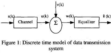
Consider an i.i.d. M-ary symbol sequence { Sk} is being transmitted through a dispersive channel h
(see Figure 1). When the channel transfer func- tion is linear, the output of the channel is the con- volution of the input sequence s k with h (U = s k
rupted by zero-mean Gaussian noise v. The out- put
of
the channel isw
= U+
v. The last m se- quences from w are taken as the input to the MPNN equalizer to restore the original signal.Channel Equalizer
Figure 1: Discrete time model of data transmission system
2.2. The Complex-valued MPNN Equalizer
The training of the MPNN requires only a one- pass training. During training, the network stores the training input vectors as centers of the net- work. These centers are assigned the values of
the desired output.
During classification, the "closeness" of a test input vector to each of the centers is determined via the kernel function. The output associated with the center closest to the input vector hence is the most likely output. It is said, therefore, that the network approximates an optimal Bayesian solution.
In equalization, the input, x, is taken as the last m sequence of the channel output.
xi =[wi wi-l
...
wi-,pSuppose y is the output to be estimated. Using a statistical model, vector x can be treated as ran- dom variable with a conditional probability of x
given y. During training the a priori distribution of y is specified based on what is known about y. It is then possible to obtain the conditional distri- bution of y given x. During classification phase, current data updates are used to yield posterior information about y.
Specht [6] has given the general regression equation of the scalar output y given an input vec- tor random variable x as expressed by (2).
Where p(x, y) is the joint continuous probability density function. This is estimated a posteriori
from the training set (xn, yn).
The equation is derived via a semiparametric technique using the Parzen-Rosenblatt density
estimator [7]. The key to this formulation is the kernel function, which has the underlying proper- ties associated with a probability density function. The final estimator equation is given in
(3),
which includes a clustering variable Zi. Without center clustering, the equation is also known as the Na- daraya-Watson Regression Estimator [7]. The kernel function shown in (4), has been formulated to accommodate for complex input vectors and complex outputs.With the m-dimensional complex vector input x
and complex output y implementing a mapping {f :
cN
+C}, the transfer function iswhere the Kernel function is
-[X-ci]H[X-Ci]
)
(4)20;
ai
(x, c i , 0) = expx
x
E CN is the input vector to the network with complex membersc, c, E CN is the center or mean vector for class i
in the input space
0, sigma is a real valued smoothing parameter
y, y, E C is the weight / output relating to center
C,
M is the total number of unique centers
Z, is the number of input training vector associ- ated with center c,
[.IH
denotes Hermitian operator (or conjugate transpose)Figure 2: Basic MPNN Architecture
each center normalized by the sum of the output of the basis function scaled by Z,.
2.3. Unsupervised Clustering of Centers
Learning involves the clustering of centers c, and the assignment of an appropriate weight y, and smoothing parameter 0, to each center.
The clustering method is similar to the k-means clustering. Close centers that are mapped to the same output are clustered together to form one new center. The location of the new center is the mean of all the centers being clustered. The total number of centers belonging to this new center is
Z,. As a result, a smaller network size can be re- alized
Define a parameter, Rx, called the radius of in- fluence. Training starts with the first training pair
{xl, yi} and establishing a center c1 at x, with a corresponding weight of y,. Given n training data pairs, the pseudo-code for the clustering method is as follows:
( Z i - l)cpld
+
xi CY" =Zi
else
z y
=1ci
= x i
end end
When all training data have been passed, training is completed.
3.
Complex Stochastic Gradient Adap-
tation
This section of the paper deals with adapting the
MPNN equalizer to slowly time varying channels. The equalizer is in decision directed (DD) mode. The output of the equalizer is compared to its closest signal constellation. The difference is the error. The parameters of the equalizer are adjusted to this error term.
For convenience let us rewrite the estimation equation and denote the numerator term as 'b' and the denominator term as 'a'.
Real and imaginary term of a variable are denoted by the subscript R and I respectively.
The error term E(k) is complex.
The objective J is to minimize the square of both the real and the imaginary error components E(k).
(9)
J is a non-constant real-valued function. Its com- plex derivative is not defined. We can however calculate its gradient with respect to the net- work's free parameters (yi, G, 0:) by using the following equations.
z i q
(X,Ci, 0;)a 'a,"
'i.k+l = 'i,k +pu,
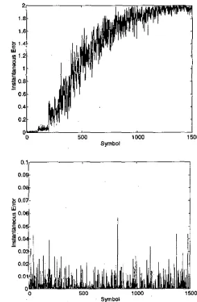
p . , , ~ - ~ , n - are learning rates for weights, The performances of a complex RBFN and a
J . 0 I
smoothing parameters and centers respec- MPNN were adapts- tion (Figure 4). The methods of a complex RBFN are detailed in [8].
The symbols in Figure 4 and Figure 5 were given sequentially with time. The initial symbols tively
re(.) denotes real operator
im(.) denotes imaginary operator
were the results of received signals at the starting positions. Consequent symbols were the result of without loss Of generality, the Source signal, s(k), received signals having drifted.
were 4 - Q m Symbols. The constellation of S(k) Initially, the parameters of the RBFN had been
were ( sl=l+j ; s2=l-j ; s3=-l+j ; s4=-1-j
I.
The tuned to give an almost perfect equalization slowly time varying channel had a transfer func- (without any miss-classification). This can be tion: observed in Figure 4a. For the first 100 symbolsOr so the rate was low' The MPNN trained
only with the clustering technique also gave an almost perfect equalization.
4.
Simulation
Results
H(z) = (1- j0.03434)
+
(0.5+
0.013+
j0.2912+ j0.007t)z-'(22) where t = k / baud rate
The non-line&y was modeled by a third order ve
For the
RBFN,
as the location Of the receivedsignal drifted from its original position, the input Volterra non-linearity and the noise was ad
of the equalizer was no longer close to any cen- ters. The overall output of the radial basis func- tions quickly converged to zero and produced Gaussian white noise
w(k) = u ( k ) +0.2u2 ( k ) +0.1u3 ( k ) +v(k) ( 2 3 )
A plot of the received symbols is shown in Fig- ure 3a, taking into account the non-linearity, the noise and the time varying component. Due to the time varying component in the transfer func- tion, the location of the received signals moved from starting positions indicated by '0' to posi-
tions indicated by 'x' (Figure 3b).
errors of 2 (Figure 4a). The MPNN o n t h e other hand, measures the relative distance of a drifted input to all centers, therefore it remains a good Bayesian estimator despite the actual drift of channel states from the centers. It is shown in Figure 4b that MPNN retains its ability to equal- izer the channel. Please note that the vertical scales in Figure 4a and 4b are different.
1
. * l o / * , .
Figure 3a, 3b: Non-linear channel with time-varying transfer functions (a) actual received signals with noise
00
variance o2 = 0.03 (b) locations Symbol 0 1
drifted from starting position
position marked by 'x' 0 0
The dimension of the input of the equalizer, m, is chosen to be 2 and the noise variance to be 0.03. 300 samples of random training data were found to be adequate to train the network.
The channel characteristic was continuously changing. New errors were introduced at any time induced by the slowly drifting channel states. Therefore, the instantaneous error can best represent the effectiveness of the equalizer. The error was measured as the sum of squared dis- tance of both real and imaginary parts from the original symbol.
1
I
Figure 4a, 4b: Comparison between RBFN and MPNN
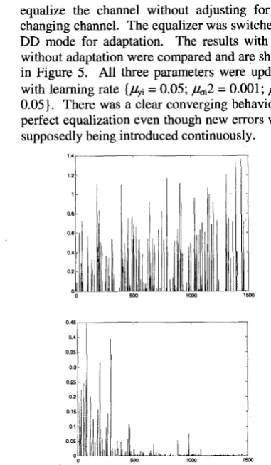
For a more severe case where the noise vari- ance
d
was 0.05 the MPNN could no longer equalize the channel without adjusting for the changing channel. The equalizer was switched to DD mode for adaptation. The results with and without adaptation were compared and are shown in Figure 5. All three parameters were updated with learning rate [hi = 0.05; b 2 = 0.001 ; Ai = 0.05). There was a clear converging behavior to perfect equalization even though new errors were supposedly being introduced continuously.1 08 0 6 0 4 0 2 0
0 500 1500
0.46,
,
I0.35
0,411
I
0.3 0.25 0.2 0.15 0.1 om 0
0 1wO ism
Figure 5a, 5b: Application of complex MPNN adapta- tion algorithms on non-linear drifting channel states
(a) without adaptation (b) adapting network
5.
Conclusion
In the simulation, MPNN was tested on a low- order, non-linear and slowly time-varying chan- nel and has exhibited good performance. For higher order channels with greater signal alphabet size, the system can suffer from the curse of di- mensionality requiring a great number of centers. A center reduction technique for the MPNN is proposed in [9] to tackle this problem.
Good tracking behavior of the MPNN equalizer was demonstrated for slowly drifting channel states. However, as with all adaptive systems, the parameter learning rates must be chosen so that they are small enough for the system to converge and are large enough so that the rate of adaptation
is greater than the rate change.
6. References
[ 11 G.Gibson, S.Siu and C.Cowan, “Multilayer Perceptron Structures Applied to Adaptive Equalisers for Data Communications”, in
Proc. of ZCASSP’89, pp. 11 83-1 186, Glas-
gow, Scotland, May 1989.
[2] S.Chen, B.Mulgrew and P.M.Grant, “A Clus- tering Technique for Digital Communications Channel Equalization Using Radial Basis Function Networks”, ZEEE Trans. Neural
Networks, vol. 4, no. 4, pp. 570-579, 1993.
31 A.Zaknich, “Introduction to the Modified Probabilistic Neural Network for General Signal Processing Applications”, ZEEE Trans.
Signal Processing, vol. 46., no. 7, pp. 1980-
1990, July 1998.
41 A.Zaknich, C.deSilva and Y.Attikiouze1, “The Probabilistic Neural Network for Non- linear Times Series Analysis“, in Proc. ZEEE
Znt. Joint Con$ Nerual Networks (WCNN),
Singapore, Nov. 1991.
[5] D.F.Specht, “Probabilistic Neural Networks”, Int. Neural Network Soc., Neural Networks,
[6] D.F.Specht, “A General Regression Neural Network”, ZEEE Trans. Neural Networks,
V01.2, Nov. 1991.
[7] S.Haykin, Neural Networks: A Cornprehen-
sive Foundation, 2nd Ed, Prentice-Hall, 1999.
[8] S.Chen, P.M.Grant,S.McLaughlin and B .Mulgrew, “Complex-valued Radial Basis Function Networks”, ZEEE Third Intema- tional Conference on Artificial Neural Net-
works, pp. 148-152, 1993.
[9] J.Young, A.Zaknich and Y.Attikiouze1, “Cen- ter Reduction Algorithm for the Modified Probabilistic Neural Network Equalizer”, to appear in ZJCNN 2001.