Vol. 12, No. 1, 2020 Article ID IJIM-1070, 12 pages Research Article
Solving a Joint Availability-Redundancy Optimization Model with
Multistate Components and Metaheuristic Approach
A. H. Borhani Alamdari∗, M. Sharifi †‡
Received Date: 2017-05-07 Revised Date: 2018-11-02 Accepted Date: 2019-06-22
————————————————————————————————–
Abstract
Redundancy allocation problem (RAP) is one of the most important and applicable problems in reliability area. This problem aims to find the optimal configuration of system components in order to optimize system reliability under some constraints. In classical model, the system component states are binary, i.e., each component is whether working or failed. In new research studies, the components are considered as multistate components, i.e., each component may have some working states ranging from full performance to completely fail. In this paper, we work on an RAP with multistate components and the performance rate of each working state may increase by spending technical and organizational activities costs. Because RAP belongs to Np-hard problems, we used Genetic Algorithm (GA) and Simulated Annealing (SA) for solving the presented problem and the Universal Generating Function (UGF) for calculating system reliability.
Keywords: Reliability optimization; Redundancy allocation problem; Multistate components; univer-sal generating function; Genetic algorithm.
—————————————————————————————————–
1
Introduction
R
AIn their model, the system has series-parallelP1was introduced by Fyffe et al. [6] in 1968. configuration with active redundancy strategy and each subsystem possesses identical compo-nents. Table 1 contains some research studies in this area. In this paper, we presented an RAP with multistate components. The performance rate of component working states may increase∗Department of Industrial and Mechanical Engineering,
Qazvin Branch, Islamic Azad University, Qazvin, Iran.
†Corresponding author. [email protected],
Tel:+98(912)2825776.
‡Department of Industrial and Mechanical Engineering,
Qazvin Branch, Islamic Azad University, Qazvin, Iran. 1
Redundancy Allocation Problem
by some technical activities. These activities change the component specifications and increase the probability of working state and decrease the probability of failed state. For calculating sys-tem reliability, we used UGF2. In 1992, Chern [2]
proved that RAP belongs to Np-hard problems, so we used GA3and SA4for solving the presented problem. This paper was divided into five tions. The model is presented in the second sec-tion. The third sections deals with the solving method. A numerical example is presented in the fourth section and the final section is devoted to conclusion and further studies.
2
Universal Generating Function 3
Genetic Algorithm 4
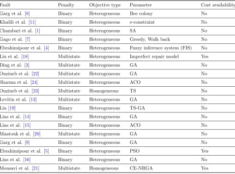
Table 1: Some Related Research Studies on RAP.
Fault Penalty Objective type Parameter Cost availability Garg et al. [8] Binary Heterogeneous Bee colony No
Khalili et al. [11] Binary Heterogeneous e-constraint No Chambari et al. [1] Binary Heterogeneous SA No Gago et al. [7] Binary Heterogeneous Greedy, Walk back No Ebrahimipour et al. [4] Binary Heterogeneous Fuzzy inference system (FIS) No Liu et al. [18] Multistate Heterogeneous Imperfect repair model Yes Ding et al. [3] Multistate Heterogeneous GA No Ouzineb et al. [22] Multistate Heterogeneous GA No Sharma et al. [24] Multistate Heterogeneous ACO No Ouzineb et al. [23] Multistate Homogeneous TS No Levitin et al. [13] Multistate Heterogeneous GA No Liu [19] Binary Heterogeneous TS-GA No Lins et al. [14] Binary Heterogeneous GA No Lins et al. [15] Binary Heterogeneous ACO No Maatouk et al. [20] Multistate Heterogeneous GA No Garg et al. [9] Binary Heterogeneous GA No Ebrahimipour et al. [5] Binary Heterogeneous PSO Yes Lins et al. [16] Binary Heterogeneous GA No Mousavi et al. [21] Multistate Homogeneous CE-NRGA Yes
2
Problem definition
In this paper, we work on an RAP with ssubsystems that are serially connected together. The problem aims to attribute the optimal allo-cated components to each subsystem under bud-get and weight constraints. The components are multistate and the probability of the working states can be increased by spending money.
2.1 Assumptions
• The system contain S subsystems that are connected serially,
• The components of each subsystem are par-allel,
• The components are multistate,
• The components are nonreplicable,
• The system parameters are deterministic,
• The components failures are independent and the failure of one component has no ef-fect on system performance individually,
• Different types of components are available for allocating to each subsystem,
• The components of each subsystem are iden-tical, and
• The components states p.d.f can be changed.
2.2 Nomenclatures
i: Subsystems index, i= 1,2, . . . , S
S: Number of subsystems,
j: Components type index, j= 1,2, . . . , Ti,
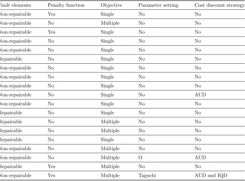
Table1. Continue
Fault elements Penalty function Objective Parameter setting Cost discount strategy
Non-repairable Yes Single No No
Non-repairable No Multiple No No
Non-repairable Yes Single No No
Non-repairable No Single No No
Non-repairable No Single No No
Repairable No Single No No
Non-repairable No Single No No
Non-repairable No Single No No
Non-repairable No Single No No
Non-repairable No Single No AUD
Non-repairable No Single No No
Repairable No Single No No
Repairable No Multiple No No
Repairable No Multiple No No
Repairable No Single No No
Non-repairable No Multiple No No
Non-repairable No Multiple O AUD
Repairable Yes Multiple No No
Non-repairable Yes Multiple Taguchi AUD and IQD
Table 2: GA parameter levels and optimal solutions.
Optimal solution Upper bound Lower bound Parameters
50 100 50 npop
0.5697 0.7 0.4 pc
0.2051 0.3 0.1 pm
Table 3: SA parameter levels and optimal solutions.
Optimal solution Upper bound Lower bound Parameters
16 20 10 nM ove
10 100 10 T0
0.1 0.3 0.1 M u0
xij : Number of j st component type allocated to
subsystem i,
zijk: Binary variables: if in subsystem i, for
Table 4: Price of components.
Component types
1 2 3 4
Subsystems 1 18 13 20 18
2 19 16 15 20
3 11 20 18 17
4 20 20 11 10
5 16 11 14 19
6 11 20 20 20
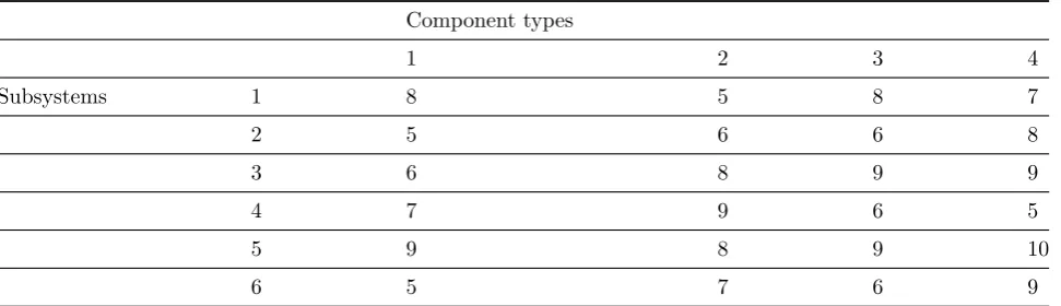
Table 5: Weight of components.
Component types
1 2 3 4
Subsystems 1 8 5 8 7
2 5 6 6 8
3 6 8 9 9
4 7 9 6 5
5 9 8 9 10
6 5 7 6 9
performance level is equal 1,
αijk: Decreasing amount of state probability in
subsystem i, for component type j, in state k,
βijk: Increasing amount of state probability in
subsystem i, for component type j, in state k,
fα
ijk: Cost of decreasing state probability in
sub-systemi, for component typej, in statek,
fijkβ : Cost of increasing state probability in sub-systemi, for component typej, in statek,
γjk : Maximum amount of decreasing state
prob-ability for component typej, in statek,
φjk : Maximum amount of increasing state
proba-bility for component typej, in statek,
cij : Cost of component typej in subsystemi,
C: Available budget,
wij : Weight of component type j in subsystem i,
C: Total acceptable system weight,
Pijk: Probability of statekfor the component type
j in subsystemk.
2.3 Mathematical model
M ax R(t) =
s ∑
i=1
Ri(t) (2.1)
S.t:
∑
i ∑
j
cij.xij + ∑
i ∑
j m∑(j)
k=1
αijk.fijkα
+∑
i ∑
j m∑(j)
k=1
βijk.fijkβ +≤C (2.2)
Table 6: Weight of components
State
1 2 3
C-type 1 C-type 2 C-type 3 C-type 4 C-type 1 C-type 2 C-type 3 C-type 4 C-type 1 C-type 2 C-type 3 C-type 4
4 4 4 4 4 1 4 3 5 4 5 1
4 1 2 4 4 3 2 1 2 3 2 1
4 2 5 1 2 5 3 1 5 2 4 3
2 1 1 3 4 2 4 2 2 5 4 4
4 1 3 3 4 3 5 5 1 3 2 5
1 5 2 4 1 2 5 2 2 3 3 1
Table 7: Cost of increasing the probability of the states
State
1 2 3
C-type 1 C-type 2 C-type 3 C-type 4 C-type 1 C-type 2 C-type 3 C-type 4 C-type 1 C-type 2 C-type 3 C-type 4
3 2 4 1 1 1 1 3 3 3 2 2
3 3 4 5 5 2 2 1 1 1 5 3
1 1 3 3 1 2 1 5 2 5 2 1
2 4 1 5 4 5 1 4 1 5 1 1
1 2 2 1 5 3 5 2 1 3 4 5
4 4 5 3 5 5 3 3 2 3 2 5
∑
i ∑
j
wij.xij ≤W (2.4)
Pijk′ =Pijk.(1 +αijk−βijk) ; ∀i, j, k (2.5) Ti
∑
j=i
Nij ≥1; ∀i= 1,2, . . . , S (2.6)
Pijk′′ = P ′
ijk ∑
k
Pijk′ ; ∀i, j, k (2.7)
αijk ≤zijk.γjk; ∀i, j, k (2.8)
βijk≤(1−zijk).φjk;∀i, j, k (2.9)
xij ≥0 (2.10)
zijk ={0,1} (2.11)
0≤αijk ≤1 (2.12)
0≤βijk≤1 (2.13)
Eq. (2.1) is the objective function that maxi-mizes system reliability. Eqs (2.2) and (2.3) are the system budget and weight constraints. Eq. (2.5) determines the effects of increasing and de-creasing policies of system states probabilities. Eq. (2.6) ensures that each subsystem contains at minimum one component. Eq. (2.7) ensures that sum of the system states probabilities are equal one. Eqs (2.8) and (2.9) make a balance between increasing and decreasing state’s prob-abilities and the Eqs (2.10) to (2.13) define the variables conditions.
3
Solving method
In this paper, UGF and GA have been used for calculating the system reliability, and for solving the presented model, respectivel.
3.1 UGF method
Ushakov [25] presented a method for calculat-ing the reliability/availability of a MSS5, which is called UGF. This method aims to reduce the calculation complexity of MSS reliability. It has been used for calculating the reliability of the sys-tem in this paper. Lisniaski and Levitin [17] pre-sented more information about this method.
3.2 Genetic algorithm
In 1975, Holland [10] from Michigan University presented the basic ideas of GA. This algorithm is based on human genetic and its steps are as follows:
1. Producing n chromosomes (each chromo-some represents a solution) called initial pop-ulation,
2. Calculating the fitness function of each chro-mosome,
3. Producing the offspring by deploying three operators:
5
Table 8: States probabilities
State
1 2 3
C-type 1 C-type 2 C-type 3 C-type 4 C-type 1 C-type 2 C-type 3 C-type 4 C-type 1 C-type 2 C-type 3 C-type 4 0.6098 0.4709 0.3104 0.2607 0.283 0.2478 0.2284 0.2783 0.1071 0.2814 0.4612 0.4611 0.5015 0.5101 0.5946 0.2142 0.1964 0.1186 0.2588 0.0835 0.302 0.3713 0.1466 0.7024 0.3028 0.3607 0.4470 0.5848 0.1543 0.5065 0.3036 0.3684 0.5429 0.1328 0.2495 0.0469 0.3972 0.2083 0.3830 0.1607 0.5649 0.5392 0.1825 0.2222 0.0379 0.2525 0.4345 0.6171 0.2908 0.3666 0.3269 0.3870 0.1779 0.1983 0.3165 0.1944 0.5312 0.4351 0.3566 0.4186 0.2360 0.4475 0.3466 0.1299 0.4266 0.0933 0.4199 0.3388 0.3374 0.4592 0.2335 0.5312
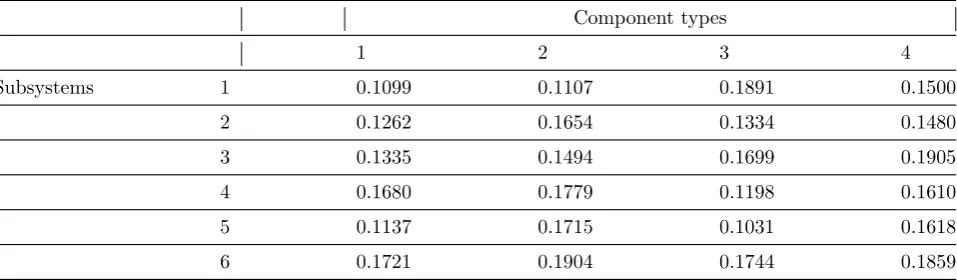
Table 9: Cost of decreasing the probability of the states (for all states are equal).
Component types
1 2 3 4
Subsystems 1 0.1099 0.1107 0.1891 0.1500
2 0.1262 0.1654 0.1334 0.1480
3 0.1335 0.1494 0.1699 0.1905
4 0.1680 0.1779 0.1198 0.1610
5 0.1137 0.1715 0.1031 0.1618
6 0.1721 0.1904 0.1744 0.1859
Table 10: Cost of decreasing the probability of the states (for all states are equal).
Component types
1 2 3 4
Subsystems 1 0.1099 0.1107 0.1891 0.1500
2 0.1262 0.1654 0.1334 0.1480
3 0.1335 0.1494 0.1699 0.1905
4 0.1680 0.1779 0.1198 0.1610
5 0.1137 0.1715 0.1031 0.1618
6 0.1721 0.1904 0.1744 0.1859
(a) Crossover,
(b) Mutation,
(c) Elitism,
4. Replacing the offspring with parents
3.3 Solution encoding
The problem chromosome contains fourxi×j,
αi×j×k,βi×j×k and zi×j×k matrixes. Definitions
of these matrixes are the same as presented in
2.2. The pseudo-code of GA is presented in Fig. 1.
3.4 Simulated Annealing
Table 11: Maximum acceptable increasing of states probabilities (for all states are equal).
Component types
1 2 3 4
Subsystems 1 0.1805 0.1490 0.1060 0.1818
2 0.1577 0.1168 0.1682 0.1818
3 0.1183 0.1979 0.1042 0.1722
4 0.1240 0.1713 0.1071 0.1150
5 0.1887 0.1500 0.1522 0.1660
6 0.1029 0.1471 0.1097 0.1519
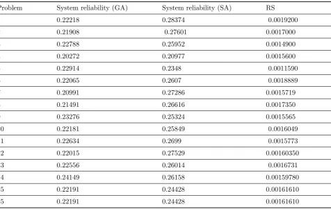
Table 12: Optimal solutions of the problems.
Problem System reliability (GA) System reliability (SA) RS
1 0.22218 0.28374 0.0019200
2 0.21908 0.27601 0.0017000
3 0.22788 0.25952 0.0014900
4 0.20272 0.20977 0.0015600
5 0.22914 0.2348 0.0011590
6 0.22065 0.2607 0.0018889
7 0.20991 0.27286 0.0015719
8 0.21491 0.26616 0.0017350
9 0.23276 0.25324 0.0015565
10 0.22181 0.25849 0.0016049
11 0.22634 0.2699 0.0015773
12 0.22015 0.27529 0.00160350
13 0.22556 0.26014 0.0016731
14 0.24149 0.26158 0.00159780
15 0.22191 0.24428 0.00161610
15 0.22191 0.24428 0.00161610
state, the old solution stays or is replaced by a new one. In both situations, the result again in-troduces it to a predefined neighborhood and be continued until algorithm meets stop condition. The pseudo-code of SA is presented in Fig. 2.
3.5 Parameter tuning
For parameter tuning of GA, we used RSM6. The GA and SA parameter levels and optimal solu-tions of parameter are presented in Tables 2 and 3.
The non-linear regression model for GA and
6
Figure 1: Pseudo-code of Genetic Algorithm.
SA parameters are as follows:
R(t)GA =0.129724−0.00623639×npop
+ 0.464773×pc+ 1.91017×pm
+ 3.63922e−005×npop×npop −0.246438×pc×pc
−2.87848×pm×pm + 0.001307×npop×pc −0.0008845×npop×pm −1.21258×pc×pm
Figure 2: Pseudo-code of simulated annealing.
R(t)SA=0.196733−0.0152087×N move −0.00141701×T0
−0.32329×M u0−0.000396208
×N move×N move
+ 1.10607e−006×T0×T0+ 1.70698
×M u0×M u0
+ 5.33389e−005×N move×T0
−0.0333775×N move×M u0
−0.00124583×T0×M u0
4
Numerical example
have three different working states. The upper bound of system weight considered 100 and the available budget is 1000. Also the minimum sys-tem performance was considered 10. The other parameters of example are presented in tables 4 to 10. Considering the presented parameters, 15 different problems are solved with GA and SA and the optimal solutions are presented in Table 11. In this 15 problem, the price of component type 1 for subsystem 1 is considered as different.
The optimal values of the problem number 10 are presented as follows:
xGA =
0 0 0 1 0 0 0 1 1 0 0 0 0 1 0 0 0 0 1 0 1 0 0 0
αGA−state1 =
0 0 0 0
0 0 0 0
1 0 0 0.1283
0 0 0
0.1029 0 0 0
0 0 0 0
αGA−state2 =
0 0 0 0.1500
0 0 0 1
0.1219 0.0456 0 0.1123 0 0.1258 0.0258 0 0 0 0.1031 0.0028 0.1709 0.0691 0 0
αGA−state3 =
0 0.0868 0 0.1268 0.0545 0 0.615 0.1038 0.0548 0 0.1048 0
0 0.1675 0.0699 0 0.389 0.1027 0.0638 0.0016 0.1423 0.0762 0 0
βGA−state1 =
0.1759 0.0098 0.0281 0.1660 0.0751 0.1168 0.0094 0.1759 0.0618 0.1559 0.0247 0 0.0724 0 0.1071 0.0290
0 0.0139 0.1196 0.0327 0.0573 0.1471 0.0334 0.0066
βGA−state2 =
0.1404 0.1385 0.0914 0 0.0340 0.1168 0.1426 0.0570
0 0 0.0137 0
0.0190 0 0 0
0.1189 0 0 0
0 0 0.0684 0.0995
BGA−state3=
0.1692 0 0.1040 0
0 0.0416 0 0
0 0 0 0
0.0605 0 0 0.0126
0 0 0 0
0 0 0.0797 0.1202
zGA−state1 =
0 0 0 0 0 0 0 0 0 0 0 1 0 0 0 0 1 0 0 0 0 0 0 0
zGA−state2 =
0 0 0 1 0 0 0 0 1 1 0 1 0 1 1 1 0 0 1 1 1 1 0 0
zGA−state3 =
0 1 0 1 1 0 1 1 1 1 1 1 0 1 1 0 1 1 1 1 1 1 0 0
xSA=
0 0 1 0 0 0 0 1 0 1 0 0 0 0 0 1 1 0 0 0 0 0 0 1
αSA−state1 =
0 0.0970 0 0
0 0.0618 0 0
0 0 0.1046 0
0 0 0 0
0 0 0 0
0.0813 0 0 0
αSA−state2 =
0 0 0.1891 0
0.0632 0 0 0.1480 0.0884 0.1494 0.0258 0 0.1680 0 0 0.1061
0.1137 0 0 0
0 0 0 0
αSA−state3 =
0 0 0.1129 0
0 0 0.1334 0.1480 0.0919 0.1494 0.1284 0.1905
0 0 0 0.1610
0.1137 0.0759 0 0.1046 0 0 0.0267 0.1440
βSA−state1=
0.0689 0 0.0965 0.0661 0.0375 0 0.0124 0.1805 0.1018 0.1979 0 0.1253 0.1146 0.1621 0.0208 0.0694 0.1221 0.0417 0.0209 0.0349 0 0.1471 0.0413 0.1280
βSA−state2=
0.0015 0.0208 0 0.0964
0 0 0 0
0 0 0 0.0794
0 0.0105 0.0834 0 0 0.1274 0.1385 0.0536
0.0964 0 0 0
BSA−state3 =
0.1116 0 0 0.1112
0 0 0 0
0 0 0 0
0.1122 0 0.1054 0
0 0 0.0604 0
0.0964 0.0685 0 0
zSA−state1 =
0 1 0 0 0 1 0 0 0 0 1 0 0 0 0 0 0 0 0 0 1 0 0 0
zSA−state2 =
0 0 1 0 1 0 1 1 1 1 1 0 1 0 0 1 1 0 0 0 0 0 1 0
zSA−state3 =
0 1 1 0 0 0 1 1 1 1 1 1 0 1 0 1 1 1 0 1 0 0 1 1
And the convergence diagram of GA and SA for this solution is presented in Fig. 3 and 4.
Figure 3: Convergence diagram of GA for prob-lem No. 10..
Figure 4: Convergence diagram of SA for prob-lem No. 10.
5
Conclusion and further
stud-ies
We propose some topics for future studies:
• Presenting a multi-objective RAP,
• Solving the presented problem for time-dependent component failure rate,
• Considering the components as repairable,
• Using other metaheuristic algorithm and comparing the results.
References
[1] A. Chambari., An efficient simulated an-nealing algorithm for the redundancy allo-cation problem with a choice of redundancy strategies, Reliability Engineering & System
Safety 11 (2013) 158-164.
[2] M. S. Chern, On the computational complex-ity of reliabilcomplex-ity redundancy allocation in a series system, Operations research letters 15 (1992) 309-315.
[3] Y. Ding, A. Lisnianski, Fuzzy universal gen-erating functions for multi-state system reli-ability assessment, Fuzzy Sets and Systems
159 (2008) 307-324.
[4] V. Ebrahimipour, S. Asadzadeh, A. Azadeh, An emotional learning-based fuzzy inference system for improvement of system reliability evaluation in redundancy allocation
prob-lem, The International Journal of Advanced
Manufacturing Technology 11 (2013) 1-16.
[5] V. Ebrahimipour, M. Sheikhalishahi, Appli-cation of multi-objective particle swarm op-timization to solve a fuzzy multi-objective reliability redundancy allocation problem,
in Systems Conference (SysCon), 2011
IEEE International, (2011) IEEE.
[6] D. E. Fyffe, W. W. Hines, N. K. Lee, System reliability allocation and a computational al-gorithm, IEEE Transactions on Reliability
17 (1968) 64-69.
[7] J. Gago, Exact cost minimization of a series-parallel reliable system with multiple com-ponent choices using an algebraic method,
Computers & Operations Research 40 (2013)
2752-2759.
[8] H. Garg, M. Rani, S. Sharma, An efficient two phase approach for solving reliability re-dundancy allocation problem using artificial bee colony technique, Computers &
Opera-tions Research 40 (2013) 2961-2969.
[9] H. Garg, S. Sharma, Multi-objective reliability-redundancy allocation problem using particle swarm optimization,
Com-puters & Industrial Engineering 64 (2013)
247-255.
[10] J. H. Holland, Adaptation in natural and artificial systems, An introductory analysis with application to biology, control and
artifi-cial intelligence, Ann Arbor, MI: University
of Michigan Press, (1975).
[11] K. Khalili Damghani, A. R. Abtahi, M. Ta-vana, A Decision Support System for Solv-ing Multi Objective Redundancy Allocation Problems, Quality and Reliability
Engineer-ing International 30 (2014) 1249-1262.
[12] S. Kirkpatrick, C. D. Gelatt, M. P. Vecchi, Optimization by simulated annealing, sci-ence 220 (1983) 671-680.
[13] G. Levitin, Reliability of series-parallel sys-tems with random failure propagation time,
IEEE Transactions on Reliability 62 (2013)
637-647.
[14] I. D. Lins, E. L. Droguett, Redundancy al-location problems considering systems with imperfect repairs using multi-objective ge-netic algorithms and discrete event simu-lation, Simulation Modelling Practice and
Theory 19 (2011) 362-381.
[15] I. Lins, E. Droguett, Multiobjective opti-mization of redundancy allocation problems in systems with imperfect repairs via ant colony and discrete event simulation, in Proceedings of the European Safety &
Relia-bility Conference (ESREL). Valencia, Spain,
(2008).
[16] I. D. Lins, E. L. Droguett, Multiobjec-tive optimization of availability and cost in repairable systems design via genetic algorithms and discrete event simulation,
[17] A. Lisniaski, G. Levitin, Multi-state sys-tem reliability: assessment,in Optimization
and Application, World Scientific Singapore,
(2003).
[18] Y. Liu, A joint redundancy and imperfect maintenance strategy optimization for multi-state systems, IEEE Transactions on
Reli-ability 62 (2013) 368-378.
[19] G. S. Liu, Availability optimization for re-pairable parallel-series system by applying Tabu-GA combination method. in Industrial Informatics (INDIN), (2012)10th IEEE
In-ternational Conference on. 2012. IEEE.
[20] I. Maatouk, E. Chtelet, N. Chebbo, Avail-ability maximization and cost study in multi-state systems, in Reliability and
Maintainability Symposium (RAMS), 2013
Proceedings-Annual. (2013). IEEE.
[21] S. M. Mousavi, Two tuned multi-objective meta-heuristic algorithms for solving a fuzzy multi-state redundancy allocation problem under discount strategies, Applied
Mathe-matical Modelling 39 (2015) 6968-6989.
[22] M. Ouzineb, M. Nourelfath, M. Gendreau, A heuristic method for non-homogeneous redundancy optimization of series-parallel multi-state systems, Journal of Heuristics
17 (2011) 1-22.
[23] M. Ouzineb, M. Nourelfath, M. Gendreau, Tabu search for the redundancy allocation problem of homogenous series parallel multi-state systems, Reliability Engineering &
System Safety, 8 (2008) 1257-1272.
[24] V. K. Sharma, M. Agarwal, Ant colony opti-mization approach to heterogeneous redun-dancy in state systems with multi-state components. in Reliability, Maintain-ability and Safety, 2009. ICRMS (2009). 8th
International Conference on. 2009, IEEE.
[25] I. Ushakov, Universal generating function,
Soviet Journal of Computer Systems Science
24 (1986) 118-129.
Amirhossein Borhani Alamdari was born in 1988 in Tehran, Iran. Amirhossein holds a B.Sc. degree from north Tehran branch Islamic Azad University in 2012, M.Sc. degree from Qzavin Islamic Azad University (QIAU) in 2017. His bachelor is in industrial engineering (system programming analysis trend) and his master is in industrial engineering (industrial trend). He is the commercial manager of Gabric-Parseh Company. He is also the CEO of Smart Dig-ital Marketing Company. His area of interest includes reliability engineering, combinatorial optimization.