Vol. 10, No. 2, 2018 Article ID IJIM-001061, 12 pages Research Article
An Efficient Numerical Algorithm For Solving Linear Differential
Equations of Arbitrary Order And Coefficients
S. Hatamzadeh-Varmazyar ∗†, Z. Masouri ‡
Received Date: 2017-04-27 Revised Date: 2017-09-07 Accepted Date: 2017-10-22
————————————————————————————————–
Abstract
Referring to one of the recent works of the authors, presented in [13], for numerical solution of linear differential equations, an alternative scheme is proposed in this article to considerably improve the accuracy and efficiency. For this purpose, triangular functions as a set of orthogonal functions are used. By using a special representation of the vector forms of triangular functions and the related operational matrix of integration, solving the differential equation reduces to solve a linear system of algebraic equations. The formulation of the method is quite general, such that any arbitrary linear differential equation may be solved by it. Moreover, the algorithm does not include any integration and, instead, uses just sampling of functions, that results in a lower computational complexity. Also, the formulation of this approach needs no modification when a singularity occurs in the coefficients of differential equation. Some problems are numerically solved by the proposed method to illustrate that it is much more accurate and applicable than the prior method in [13].
Keywords : Linear differential equation; Numerical algorithm; Triangular functions; Vector forms; Operational matrix of integration.
—————————————————————————————————–
1
Introduction
T
hforms of functional equations such as inte-e differential equations beside the other gral and integro-differential equations are widely used for modeling of many problems in physical science and engineering. Such models often have no analytical solution and, therefore, obtaining an approximate solution for them requires a suit-able numerical method [5, 15, 14, 23, 12, 16, 8, 20,18,21,17, 1,2,3,4,19].∗Corresponding author. [email protected]. †Department of Electrical Engineering, Islamshahr
Branch, Islamic Azad University, Tehran, Iran.
‡Department of Mathematics, Islamshahr Branch,
Is-lamic Azad University, Tehran, Iran.
An interesting numerical method for solving or-dinary linear differential equations has been pre-sented in [13]. It uses vector forms of block-pulse functions (BPFs) [22, 9] for setting up an alge-braic equations system and, finally, computing
the approximate solution. Although the
men-tioned method shows a good efficiency (especially, in view of generality), it has some drawbacks re-garding the accuracy and singularity. It is the main aim of this article to present a suitable ap-proach to overcome the disadvantages.
This article proposes a numerical method for solving linear ordinary differential equations of
arbitrary order and coefficients. For this
pur-pose, a special representation of the vector forms of triangular functions (TFs) [10] are used to
proximate the solution, its derivatives, and the equation coefficients. By using the related TFs operational matrix of integration, the TFs coeffi-cients vector of the solution and that of its vari-ous derivatives are expressed in terms of the TFs coefficients vector of the highest order derivative and the initial conditions vectors, that results in a linear system of algebraic equations. Solving this system gives the TFs coefficients vector of the highest order derivative and, accordingly, an approximate solution for the differential equation is obtained. The main advantages of the proposed method are as follows:
[•]The formulation of the method is quite
general, without limitation or restriction. Therefore, it can be used for numerically solving every linear ordinary differential equation of arbitrary order and coefficients. The accuracy of the method is high (con-siderably higher than that of the BPFs
method). The algorithm does not include
any integration and, instead, uses just sam-pling of functions, that results in a lower computational complexity. This is due to the use of orthogonal TFs set, as it uses piecewise linear approximation technique where the co-efficients are samples of the approximated function. The algorithm of BPFs method, for a normal discretization size of the prob-lem, includes a great number of integrations for setting up the algebraic equations sys-tem. The formulation of this approach needs no modification when a singularity occurs in the coefficients of differential equation. Since the method uses no integration, then there is no need to pass through the singular point, necessarily. In fact, the sampling points may easily be set up such that none of them
co-incides with the singular point. It should
be mentioned that the formulation of BPFs method needs some modification in such a case. The algorithm is simple and clear to use and can be implemented easily.
The organization of this article is as follows. A brief review on TFs and their vector forms
is provided in section 2. A special
representa-tion of TFs, introduced in [5], is surveyed in
sec-tion 3. Section 4 presents the numerical method
for solving arbitrary linear ordinary differential equations by using the special representation of TFs vector forms and the related operational ma-trix of integration. Some test problems are
nu-merically solved in section 5 by the proposed
method and the related numerical results are
given. There will be extensive varieties of
or-ders, coefficients, types, and solutions associated with the test problems to illustrate the general-ity and computational efficiency of the proposed method. The obtained results are also compared with those of the method presented in [13] to con-firm the superiority of the proposed method in this article over the BPFs method in view of ac-curacy and flexibility. Finally, conclusions will be given in section 6.
2
Review
of
triangular
func-tions [
10
]
2.1 Definition
Two m-sets of TFs are defined over the interval
[0, H) as [10]
T1i(t) = {
1−t−hih, ih⩽t <(i+ 1)h,
0, otherwise,
T2i(t) = {
t−ih
h , ih⩽t <(i+ 1)h,
0, otherwise,
(2.1)
where i= 0,1, . . . , m−1, with a positive integer value form. Also, considerh=H/m, andT1i as the ith left-handed TF and T2i as the ith right-handed TF.
Here, we assume that H = 1, so TFs are
de-fined over [0,1), and h= 1/m.
From the definition of TFs, it is clear that they are disjoint, orthogonal, and complete [10]. Also, we can write
φi(t) =T1i(t) +T2i(t), i= 0,1, . . . , m−1, (2.2) where φi(t) is theith BPF defined as
φi(t) = {
1, ih⩽t <(i+ 1)h,
0, otherwise, (2.3)
2.2 Vector forms
Consider the firstmterms of left-handed TFs and
the first m terms of right-handed TFs and write
them concisely as m-vectors:
T1(t) = [T10(t), T11(t), ..., T1m−1(t)]T,
T2(t) = [T20(t), T21(t), ..., T2m−1(t)]T,
(2.4)
where T1(t) and T2(t) are called left-handed
triangular functions (LHTF) vector and right-handed triangular functions (RHTF) vector, re-spectively.
2.3 TFs expansion
The expansion of a functionf(t) over [0,1) with respect to TFs, may be compactly written as
f(t)≃ m∑−1
i=0
ciT1i(t) + m∑−1
i=0
diT2i(t)
=cTT1(t) +dTT2(t),
(2.5)
where we may putci=f(ih) anddi=f((i+ 1)h) fori= 0,1, . . . , m−1. So, approximating a known function by TFs needs no integration to evaluate the coefficients.
2.4 Operational matrix of integration
Expressing∫0sT1(τ)τ and ∫0sT2(τ)τ in terms of TFs follows [10]:
∫ s
0
T1(τ)τ ≃P1T1(s) +P2T2(s),
∫ s
0
T2(τ)τ ≃P1T1(s) +P2T2(s),
(2.6)
whereP1m×m andP2m×m are called operational matrices of integration in TFs domain and
repre-sented as follows:
P1 = h 2
0 1 1 . . . 1 0 0 1 . . . 1 0 0 0 . . . 1
..
. ... ... . .. ... 0 0 0 . . . 0
,
P2 = h 2
1 1 1 . . . 1 0 1 1 . . . 1 0 0 1 . . . 1
..
. ... ... . .. ... 0 0 0 . . . 1
.
(2.7)
So, the integral of any function f(t) can be ap-proximated as
∫ s
0
f(τ)τ ≃
∫ s
0 [
cTT1(τ) +dTT2(τ)]τ
≃(c+d)TP1T1(s) + (c+d)TP2T2(s).
(2.8)
3
A special representation of
TFs vector forms and other
properties [
5
]
In this section, we survey a special representa-tion of TFs vector forms that has originally been introduced in [5]. Then, some characteristics of TFs are presented based on this representation.
3.1 Definition and expansion
Let T(t) be a 2m-vector defined as [5]
T(t) = T1(t)
T2(t)
, 0⩽t <1, (3.9)
whereT1(t) andT2(t) have been defined in (2.4).
Now, the expansion of f(t) with respect to TFs
can be written as
f(t)≃F1TT1(t) +F2TT2(t)
=FTT(t)
=TT(t)F,
(3.10)
whereF1 andF2 are TFs coefficients withF1i=
1. Also, 2m-vector F is defined as
F = F1
F2
. (3.11)
Now, assume that k(s, t) is a function of two
variables. It can be expanded with respect to
TFs as follows:
k(s, t)≃TT(s) K T(t), (3.12)
where T(s) and T(t) are 2m1- and 2m
2-dimensional TFs respectively, and K is a 2m1×
2m2 TFs coefficient matrix. For convenience, we
putm1 =m2 =m. So, matrix K can be written
as
K =
(K11)m×m (K12)m×m (K21)m×m (K22)m×m
, (3.13)
where K11, K12, K21, and K22 can be
com-puted by sampling of function k(s, t) at pointssi and ti such that si =ti =ih, fori= 0,1, . . . , m. Therefore,
(K11)i,j =k(si, tj), i= 0,1, . . . , m−1,
j= 0,1, . . . , m−1,
(K12)i,j =k(si, tj), i= 0,1, . . . , m−1,
j= 1,2, . . . , m,
(K21)i,j =k(si, tj), i= 1,2, . . . , m,
j= 0,1, . . . , m−1,
(K22)i,j =k(si, tj), i= 1,2, . . . , m,
j= 1,2, . . . , m.
(3.14)
3.2 Product properties
Let X be a 2m-vector which can be written as
XT = (X1T X2T) such that X1 and X2 are
m-vectors. Now, it can be concluded that [5]
T(t)TT(t)X ≃X˜T(t), (3.15)
where ˜X=diag(X) is a 2m×2mdiagonal matrix. Now, let B be a 2m×2m matrix. We have [5]
TT(t)BT(t)≃BˆTT(t), (3.16)
in which ˆB is a 2m-vector with elements equal to the diagonal entries of matrix B. Moreover, it is concluded that [5]
∫ 1
0
T(t)TT(t) t≃D, (3.17)
where Dis a 2m×2m matrix defined as
D= h 3Im×m
h 6Im×m h
6Im×m h 3Im×m
. (3.18)
3.3 Operational matrix
Expressing ∫0sT(τ)τ in terms of T(s), and from Eqs. (2.6), we can write [5]
∫ s
0
T(τ)τ ≃PT(s), (3.19)
where P2m×2m, operational matrix of T(s), is
P =
P1 P2
P1 P2
, (3.20)
in which P1 andP2 are given by (2.7).
Now, the integral of any function f(t) can be approximated as
∫ s
0
f(τ)τ ≃
∫ s
0
FTT(τ)τ
≃FTPT(s).
(3.21)
4
Numerical algorithm for
solv-ing arbitrary linear
differen-tial equations
Here, by using the mentioned representation of TFs vector forms and properties, we propose an effective numerical algorithm for solving linear differential equations of arbitrary order and co-efficients.
Let us consider a general ordinary linear dif-ferential equation, with arbitrary coefficients, of arbitrary order nas follows:
x(n)(t) +an−1(t)x(n−1)(t) +an−2(t)x(n−2)(t) +· · ·+a1(t)x′(t) +a0(t)x(t) =b(t),
with the following initial conditions:
x(t0) =α0,
x′(t0) =α1, ..
.
x(n−1)(t
0) =αn−1,
(4.23)
wherexis the unknown function, with respect to
variablet, to be determined;x(k),k= 1,2, . . . , n, is the kth derivative of x with respect to t; co-efficients ak, k = 0,1, . . . , n−1, andb are func-tions of t; andαk,k= 0,1, . . . , n−1, is a scalar. Also, without loss of generality, it is supposed thatt0 = 0.
Approximating the functions x; x(k), k =
1,2, . . . , n; ak, k = 0,1, . . . , n −1; and b with respect to TFs, using Eq. (3.10), gives
x(t)≃X0TT(t) =TT(t)X0,
x(k)(t)≃XkTT(t) =TT(t)Xk,
ak(t)≃ATkT(t) =TT(t)Ak,
b(t)≃BTT(t) =TT(t)B,
(4.24)
where them-vectorsX0,Xk,Ak, and B are TFs coefficients ofx,x(k),ak, and b, respectively.
Substituting Eqs. (4.24) into Eq. (4.22) gives
XnTT(t) +ATn−1T(t)TT(t)Xn−1 +ATn−2T(t)TT(t)Xn−2+· · · +AT1T(t)TT(t)X1
+AT0T(t)TT(t)X0 ≃BTT(t).
(4.25)
Using Eq. (3.15) follows
XnTT(t) +ATn−1X˜n−1T(t) +ATn−2X˜n−2T(t) +· · ·+AT1X˜1T(t) +A0TX˜0T(t)≃BTT(t),
(4.26)
or
XnT +ATn−1X˜n−1+ATn−2X˜n−2 +· · ·+AT1X˜1+AT0X˜0 ≃BT.
(4.27)
Transposition of both sides of Eq. (4.27) yields
Xn+ ˜Xn−1An−1+ ˜Xn−2An−2 +· · ·+ ˜X1A1+ ˜X0A0 ≃B,
(4.28)
because ˜XkT = ˜Xk,k= 0,1, . . . , n−1. Therefore, by considering ˜XkAk= ˜AkXk,k= 0,1, . . . , n−1, we get
Xn+ ˜An−1Xn−1+ ˜An−2Xn−2 +· · ·+ ˜A1X1+ ˜A0X0 ≃B.
(4.29)
On the other hand we have
∫t 0x
(n)(τ)τ =x(n−1)(t)−α n−1, ∫t
0x(n−1)(τ)τ =x(n−2)(t)−αn−2, ∫t
0x
(n−2)(τ)τ =x(n−3)(t)−α n−3, ..
. ∫t
0x′(τ)τ =x(t)−α0,
(4.30)
which results in
PTXn≃Xn−1−⃗αn−1,
PTXn−1≃Xn−2−⃗αn−2,
PTXn−2≃Xn−3−⃗αn−3, ..
.
PTX1 ≃X0−⃗α0,
(4.31) or
Xn−1 ≃PTXn+⃗αn−1,
Xn−2 ≃PTXn−1+⃗αn−2,
Xn−3 ≃PTXn−2+⃗αn−3, ..
.
X0 ≃PTX1+⃗α0,
(4.32)
in which P is the operational matrix of
integra-tion in Eq. (3.19) and ⃗αk, k= 0,1, . . . , n−1, is
an m-vector with elements equal to αk.
Equa-tions (4.32) may be rewritten as
Xn−1 ≃PTXn+⃗αn−1,
Xn−2 ≃(PT)2Xn+PTα⃗n−1+α⃗n−2,
Xn−3 ≃(PT)2Xn−1+PTα⃗n−2+⃗αn−3, ..
.
X0 ≃(PT)2X2+PTα⃗1+⃗α0.
After successive substitutions we finally obtain
Xn−1≃PTXn+α⃗n−1,
Xn−2≃(PT)2Xn+PT⃗αn−1+⃗αn−2,
Xn−3≃(PT)3Xn+ (PT)2⃗αn−1 +PTα⃗n−2+⃗αn−3, ..
.
X0 ≃(PT)nXn+ (PT)n−1⃗αn−1
+(PT)n−2⃗αn−2+· · ·+PT⃗α1+α⃗0. (4.34)
Now, we substitute Eqs. (4.34) into Eq. (4.29) and get
Xn+ ˜An−1(PTXn+⃗αn−1)
+ ˜An−2((PT)2Xn+PTα⃗n−1+⃗αn−2) + ˜An−3((PT)3Xn+ (PT)2α⃗n−1 +PT⃗αn−2+⃗αn−3)
+· · ·
+ ˜A0((PT)nXn+ (PT)n−1⃗αn−1 + (PT)n−2⃗αn−2+· · ·+PT⃗α1+α⃗0) ≃B,
(4.35)
or
Xn+ [
( ˜An−1PT)Xn+ ˜An−1α⃗n−1 ]
+ [
( ˜An−2(PT)2)Xn+ ˜An−2PT⃗αn−1
+ ˜An−2⃗αn−2 ]
+ [
( ˜An−3(PT)3)Xn+ ˜An−3(PT)2⃗αn−1
+ ˜An−3PT⃗αn−2+ ˜An−3⃗αn−3 ]
+· · ·
+ [
( ˜A0(PT)n)Xn+ ˜A0(PT)n−1α⃗n−1 + ˜A0(PT)n−2⃗αn−2+· · ·+ ˜A0PT⃗α1 + ˜A0α⃗0
]
≃B.
(4.36)
Equation (4.36) may be rewritten as
[
I+ ˜An−1PT + ˜An−2(PT)2
+ ˜An−3(PT)3+· · ·+ ˜A0(PT)n ]
Xn
≃B−
[
( ˜An−1⃗αn−1)
+ ( ˜An−2PT⃗αn−1+ ˜An−2⃗αn−2) + ( ˜An−3(PT)2⃗αn−1+ ˜An−3PTα⃗n−2 + ˜An−3⃗αn−3)
+ · · ·
+ ( ˜A0(PT)n−1⃗αn−1+ ˜A0(PT)n−2α⃗n−2 +· · ·+ ˜A0PTα⃗1+ ˜A0⃗α0)
]
.
(4.37)
Now, we replace ≃with =, and write Eq. (4.37)
in a simpler form as
GXn=W, (4.38)
in which
G=I+ n−1 ∑
r=0 ˜
Ar(PT)n−r, (4.39)
and
W =B−
n−1 ∑
k=0 n−1 ∑
r=k ˜
Ak(PT)r−kα⃗r. (4.40)
Equation (4.38) is a linear system of m
al-gebraic equations with respect to m unknowns
xn0, xn1, . . . , xnm−1, components of Xn.
Solu-tion of this system gives vector Xn. Then, form
Eqs. (4.34) we have
X0≃(PT)nXn+ (PT)n−1α⃗n−1
+ (PT)n−2⃗αn−2+· · ·+PT⃗α1+α⃗0.
(4.41)
Substituting the determined Xn into Eq. (4.41)
gives the unknown vectorX0. Hence, an
approx-imate solution for differential equation (4.22) is obtained as
x(t)≃X0TT(t). (4.42)
1. 2. 3. 4.
of Eq. (4.22) in any arbitrary bounded real inter-val. For this purpose, we assume that TFs are de-fined over arbitrary bounded interval[α, β), where
α, β ∈R. It is clear that all the properties and re-lations presented as to the TFs can be easily gen-eralized over this interval provided that T1i and
T2i, i= 0,1, . . . , m−1, are defined as
T1i(t) = {
1−t−ih−α
h , α+ih⩽t < α+ (i+ 1)h,
0, otherwise,
T2i(t) =
{t−ih−α
h , α+ih⩽t < α+ (i+ 1)h,
0, otherwise,
(4.43)
in whichh= (β−α)/m. By using the above gen-eralization, the formulation proposed in the cur-rent section can be applied in solution of the dif-ferential equation in any arbitrary bounded real interval [α, β) without needing any modification to the formulas of the presented method.
5
Test problems and numerical
results
Some test problems are numerically solved here by the proposed method in this article and the re-lated numerical results are compared with those
of the method proposed in [13]. There are
ex-tensive varieties of orders, coefficients, types, and solutions associated with the test problems given here to illustrate the generality and computa-tional efficiency of the proposed method for the solution of arbitrary linear ordinary differential equations.
The approximate results obtained by both methods for each test problem are calculated at ten points ti in the related interval [α, β) such that ti = α + ih′, where i = 0,1, . . . ,9 and
h′ = (β −α)/10. Moreover, all the results are given in the form of mean-absolute error. If, for
a given m, we obtain the approximate solution
at ten pointsti, then we can consider the mean-absolute error, related to this value of m, as fol-lows:
Em = 1 10
9 ∑
i=0
|x(ti)−xm(ti)|, (5.44)
whereEis the mean-absolute error, andxandxm
stand for the exact and approximate solutions, respectively.
In general, the numerical results obtained by both methods in solution of the considered test problems show the superiority of the proposed method in this article over the BPFs method [13] in view of accuracy and flexibility. This will be illustrated in tables1–5related to the test prob-lems.
It should be mentioned that all the computa-tions associated with both methods have been performed using MATLAB software.
Example 5.1 Numerical solution of Bessel’s equation [13]
The well-known Bessel’s equation as a linear homogeneous second-order ordinary differential equation is given by [7, 11]
t2x′′(t) +tx′(t) + (t2−ν2)x(t) = 0, (5.45)
or
x′′(t) + 1
tx
′(t) + (1−ν2
t2)x(t) = 0, (5.46)
where ν is a real constant. As a second-order
differential equation, Bessel’s equation has two
independent solutions. If ν = ℓ is an integer,
one solution defines Jℓ(t) as the Bessel function of the first kind of order ℓ, and another solution defines Yℓ(t) referred to as the Bessel function of
the second kind of order ℓ. The Bessel functions
play an important role in physical and engineer-ing problems; for instance, the Bessel function of the first kind appears in the solution of elec-tromagnetic wave equation inside circular
waveg-uides [11]. We apply both methods for
numeri-cally solving Bessel’s equation to obtain its ap-proximate solutions. The initial conditions are set such that the equation has a unique solution
Jℓ(t). The exact values ofJℓ have been extracted by MATLAB software. However, a series solution is available as [11]
Jℓ(t) = ∞ ∑
m=0
(−1)m
m! (m+ℓ)! (
t
2 )2m+ℓ
. (5.47)
Moreover
J−ℓ(t) = (−1)ℓJℓ(t),
Jℓ(−t) = (−1)ℓJℓ(t).
Table 1: Mean-absolute errors for test problem5.1(results forJ0).
m Proposed method in this article Presented method in [13]
2 2.6
e
−2 4.2e
−24 1.1
e
−2 2.1e
−28 3.9
e
−3 7.9e
−316 1.3
e
−3 3.8e
−332 3.9
e
−4 1.8e
−364 1.2
e
−4 7.9e
−4128 3.3
e
−5 3.7e
−4256 9.4
e
−6 1.9e
−4512 2.6
e
−6 9.6e
−51024 7.3
e
−7 4.8e
−5Table 2: Mean-absolute errors for test problem5.2(results forP1).
m Proposed method in this article Presented method in [13]
2 0 2.5
e
−14 0 1.2
e
−18 0 4.9
e
−216 0 2.0
e
−232 0 8.6
e
−364 0 4.2
e
−3128 0 2.1
e
−3256 0 1.0
e
−3512 0 5.1
e
−41024 0 2.5
e
−4Table 3: Mean-absolute errors for test problem5.3.
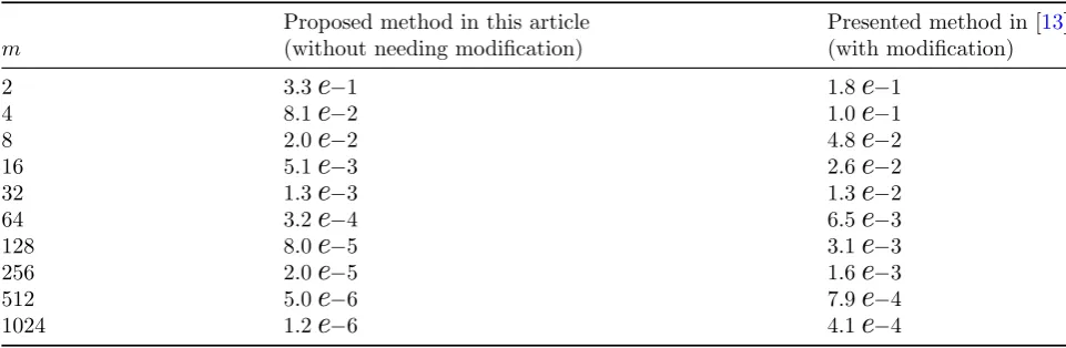
Proposed method in this article Presented method in [13]
m (without needing modification) (with modification)
2 3.3
e
−1 1.8e
−14 8.1
e
−2 1.0e
−18 2.0
e
−2 4.8e
−216 5.1
e
−3 2.6e
−232 1.3
e
−3 1.3e
−264 3.2
e
−4 6.5e
−3128 8.0
e
−5 3.1e
−3256 2.0
e
−5 1.6e
−3512 5.0
e
−6 7.9e
−41024 1.2
e
−6 4.1e
−4The following relations may be used to obtain the
derivatives of Bessel functions with respect to t
for the required initial conditions. Letting Uν(t) denote an arbitrary solution to Bessel’s equation,
we have [11]
Uν′(t) =Uν−1−
ν tUν, Uν′(t) =−Uν+1+
ν tUν.
(5.49)
Table 4: Mean-absolute errors for test problem5.4.
m Proposed method in this article Presented method in [13]
2 2.2
e
−2 1.3e
−14 5.7
e
−3 6.5e
−28 1.4
e
−3 3.2e
−216 3.6
e
−4 1.6e
−232 9.0
e
−5 8.1e
−364 2.3
e
−5 4.1e
−3128 5.7
e
−6 2.0e
−3256 1.4
e
−6 1.0e
−3512 3.5
e
−7 5.1e
−41024 8.8
e
−8 2.5e
−4Table 5: Mean-absolute errors for test problem5.5.
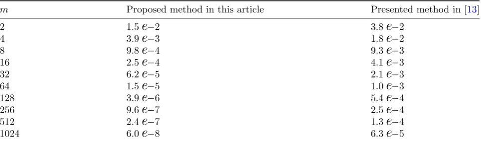
m Proposed method in this article Presented method in [13]
2 1.5
e
−2 3.8e
−24 3.9
e
−3 1.8e
−28 9.8
e
−4 9.3e
−316 2.5
e
−4 4.1e
−332 6.2
e
−5 2.1e
−364 1.5
e
−5 1.0e
−3128 3.9
e
−6 5.4e
−4256 9.6
e
−7 2.5e
−4512 2.4
e
−7 1.3e
−41024 6.0
e
−8 6.3e
−5Example 5.2 Numerical solution of Legendre differential equation [13]
The Legendre differential equation as a lin-ear homogeneous second-order ordinary differen-tial equation is given by [6]
(1−t2)x′′(t)−2tx′(t) +ν(ν+ 1)x(t) = 0, (5.50)
or
x′′(t)− 2t
1−t2x′(t) +
ν(ν+ 1)
1−t2 x(t) = 0. (5.51)
where ν is a real constant. One solution to the
Legendre differential equation defines the Legen-dre function of the first kindPν(t). Ifν =ℓis an integer, solution of the Legendre differential equa-tion results in funcequa-tionPℓ(t) known as the
Legen-dre polynomial of degree ℓ. Another solution to
this equation givesQℓ(t) referred to as the Legen-dre function of the second kind. Like the Bessel functions, the Legendre functions too have vari-ous applications in physical and engineering prob-lems; e.g., associated Legendre functions appear
in the solution of Helmholtz equation in spheri-cal coordinates [11]. The exact values of the first
six polynomialsPℓmay be calculated through the
following analytical relations [6]:
P0(t) = 1, P1(t) =t,
P2(t) = 1 2(3t
2−1),
P3(t) = 1 2(5t
3−3t),
P4(t) = 1 8(35t
4−30t2+ 3),
P5(t) = 1 8(63t
5−70t3+ 15t).
(5.52)
We apply both methods in solving the Legen-dre differential equation and set the initial condi-tions such that the equation has a unique solution
Example 5.3 Numerical solution of a third-order inhomogeneous differential equation with singular coefficients [13]
We survey in this problem the flexibility of the proposed method in solution of differential equa-tions with singular coefficients. For this purpose, let us consider the following third-order inhomo-geneous linear differential equation:
x′′′(t)− t
t2−0.64ln(t
2+ 0.64)x′′(t)
+t2sin (
1
t−0.8 )
x′(t)
+ cos(πt2)x(t) =b(t),
(5.53)
with exact solutionx(t) =t3+ sin(πt) and right side b(t) as
b(t) = 6−π3cos(πt)
− t
t2−0.64ln(t
2+ 0.64)[6t−π2sin(πt)]
+t2[3t2+πcos(πt)] sin (
1
t−0.8 )
+ cos(πt2)[t3+ sin(πt)].
(5.54)
Coefficient a1 = t2sin (
1 t−0.8
)
has an essential
singularity and coefficient a2 = −t2−t0.64ln(t2 + 0.64) has a pole-type singularity at t = 0.8 in interval [0,1).
In such a case, the BPFs method is unable to obtain an appropriate solution by its original
for-mulation, and it needs some modification [13].
However, the proposed method in this article can give a reasonable solution without any modifica-tion.
The mean-absolute errors associated with both methods in solution of test problem5.3, in
inter-val [0,1), are shown in Table 3. As mentioned
above, the BPFs method has been implemented via modification.
Example 5.4 Numerical solution of a high-order inhomogeneous differential equation with both complex solution and complex coeffi-cients [13]
We show in this problem that the proposed method is applicable in solving differential equa-tions with complex solution and/or complex coef-ficients. Let us consider an inhomogeneous linear
differential equation of order 15 as
x(15)(t) + (t3−jt2+ 1)x(10)(t)
+ (t+j)H0(2)(t)x(5)(t)
+jtsin(t2+jt)x(t) =b(t),
(5.55)
whereH0(2) is Hankel function of the second kind
of zero-order, j is imaginary unit and j2 = −1.
Assuming complex exact solution x(t) = exp(jt) for Eq. (5.55), the right side will be
b(t) =−exp(jt) {
t3+jt2
−j[H0(2)(t) + sin(t2+jt)]t
+H0(2)(t) +j+ 1 }
.
(5.56)
Both methods are applied in solving Eq. (5.55) to obtain its approximate solutions in interval [3,4).
The mean-absolute errors are given in Table 4.
Example 5.5 Numerical solution of a very high-order inhomogeneous differential equation [13]
We survey here the efficiency of the proposed method for numerical solution of very high-order differential equations. For this purpose, we con-sider the following inhomogeneous linear differ-ential equation of order 35:
x(35)(t) + tan(√|t|)x(20)(t)
+t2sin(t2)x(11)(t)
+ cos(√t4+ 1)x(t) =b(t),
(5.57)
with exact solution x(t) = exp(t) + sin(t) and right side b(t) as
b(t) = exp(t) [
1 + tan(√|t|) +t2sin(t2)
+ cos(√t4+ 1)]
+ sin(t) [
tan(√|t|) + cos(√t4+ 1)]
−cos(t) [
1 +t2sin(t2) ]
.
(5.58)
6
Conclusion
A numerical approach for solving arbitrary lin-ear ordinary differential equations was proposed in this article by using a special representation of TFs vector forms and the related operational matrix of integration. Some test problems were numerically solved by the method to illustrate its computational efficiency and to show that it is applicable in solving various types of ordinary lin-ear differential equations. In comparison with the BPFs method, we saw that the proposed method is more accurate and flexible and has no limita-tion.
References
[1] E. Babolian, Z. Masouri, S. Hatamzadeh-Varmazyar, A direct method for numerically solving integral equations system using
or-thogonal triangular functions, International
Journal of Industrial Mathematics 1 (2009) 135-145.
[2] E. Babolian, Z. Masouri, S. Hatamzadeh-Varmazyar, A set of multi-dimensional or-thogonal basis functions and its applica-tion to solve integral equaapplica-tions,International Journal of Applied Mathematics and Compu-tation 2 (2010) 032-049.
[3] E. Babolian, Z. Masouri, S. Hatamzadeh-Varmazyar, Introducing a direct method to solve nonlinear Volterra and Fredholm in-tegral equations using orthogonal triangular
functions,Mathematics Scientific Journal 5
(2009) 11-26.
[4] E. Babolian, Z. Masouri, S. Hatamzadeh-Varmazyar, New direct method to solve
nonlinear Volterra-Fredholm integral
and integro-differential equations using
operational matrix with block-pulse
func-tions,Progress In Electromagnetics Research
B 8 (2008) 59-76.
[5] E. Babolian, Z. Masouri, S. Hatamzadeh-Varmazyar, Numerical solution of nonlinear Volterra-Fredholm integro-differential equa-tions via direct method using triangular
functions, Computers & Mathematics with
Applications 58 (2009) 239-247.
[6] C.A. Balanis, Advanced Engineering
Elec-tromagnetics, Wiley, New York,1989.
[7] C.A. Balanis, Antenna Theory: Analysis and
Design, 2nd edition,Wiley, New York,1996.
[8] R. Danesfahani, S. Hatamzadeh-Varmazyar, E. Babolian, Z. Masouri, A scheme for RCS
determination using wavelet basis,
AEU-International Journal of Electronics and Communications 64 (2010) 757-765.
[9] A. Deb, G. Sarkar, S. K. Sen, Block pulse functions, the most fundamental of all
piece-wise constant basis functions, International
Journal of Systems Science 25 (1994) 351-363.
[10] A. Deb, G. Sarkar, A. Sengupta, Triangu-lar Orthogonal Functions for the Analysis
of Continuous Time Systems,Anthem Press,
London, 2011.
[11] R. F. Harrington, Time-Harmonic
Electro-magnetic Fields,IEEE Press series on
elec-tromagnetic wave theory, 2nd edition, Wiley-IEEE Press, New York, 2001.
[12] S. Hatamzadeh-Varmazyar, Z. Masouri, Nu-merical method for analysis of one-and two-dimensional electromagnetic scattering based on using linear Fredholm integral
equation models, Mathematical and
Com-puter Modelling 54 (2011) 2199-2210.
[13] S. Hatamzadeh-Varmazyar, Z. Masouri, E. Babolian, Numerical method for solving ar-bitrary linear differential equations using a set of orthogonal basis functions and
oper-ational matrix, Applied Mathematical
Mod-elling 40 (2016) 233-253.
[14] S. Hatamzadeh-Varmazyar, M.
Naser-Moghadasi, E. Babolian, Z. Masouri,
Calculating the radar cross section of the resistive targets using the Haar wavelets,
[15] S. Hatamzadeh-Varmazyar, M. Naser-Moghadasi, Z. Masouri, A moment method
simulation of electromagnetic
scatter-ing from conductscatter-ing bodies, Progress In
Electromagnetics Research 81 (2008) 99-119.
[16] S. Hatamzadeh-Varmazyar, M.
Naser-Moghadasi, E. Babolian, Z. Masouri,
Numerical approach to survey the problem of electromagnetic scattering from resistive strips based on using a set of orthogonal
ba-sis functions, Progress In Electromagnetics
Research 81 (2008) 393-412.
[17] S. Hatamzadeh-Varmazyar, Z. Masouri, A fast numerical method for analysis of one-and two-dimensional electromagnetic scat-tering using a set of cardinal functions, En-gineering Analysis with Boundary Elements
36 (2012) 1631-1639.
[18] S. Hatamzadeh-Varmazyar, Z. Masouri, A numerical approach for calculating the radar cross-section of two-dimensional perfect
elec-trically conducting structures, Journal of
Electromagnetic Waves and Applications 28 (2014) 1360-1375.
[19] S. Hatamzadeh-Varmazyar, Z. Masouri, De-termining the electromagnetic fields
scat-tered from PEC cylinders,International
Journal of Mathematics & Computation 28 (2017) 1-8.
[20] S. Hatamzadeh-Varmazyar, Z. Masouri,
Numerical expansion-iterative method for analysis of integral equation models aris-ing in one-and two-dimensional
electromag-netic scattering, Engineering Analysis with
Boundary Elements 36 (2012) 416-422.
[21] S. Hatamzadeh-Varmazyar, M.
Naser-Moghadasi, R. Sadeghzadeh-Sheikhan,
One-and two-dimensional scattering
anal-ysis using a fast numerical method, IET
Microwaves, Antennas & Propagation 5 (2011) 1148-1155.
[22] J. H. Jiang, W. Schaufelberger, Block pulse functions and their application in control
system, LNCIS, vol. 179, Springer-Verlag,
Berlin,1992.
[23] Z. Masouri, E. Babolian, S. Hatamzadeh-Varmazyar, An expansion-iterative method for numerically solving Volterra integral
equation of the first kind,Computers &
Mathematics with Applications 59 (2010) 1491-1499.
Saeed Hatamzadeh-Varmazyar,
Ph.D. in Electrical
Engineer-ing, is an Assistant Professor
at Islamshar Branch, Islamic
Azad University, Tehran, Iran.
His research interests include
computational Electromagnetics,
numerical methods for solving integral equations, electromagnetic theory, singular integral equa-tions, electromagnetic radiation and antenna,
and propagation of electromagnetic waves,
including scattering, diffraction, and etc. Dr.
Hatamzadeh-Varmazyar is the author of many research articles published in scientific journals. More details may be found on his official website
available online athttp://www.hatamzadeh.ir/
and http://www.hatamzadeh.org/.