Volume 55, 2018, Pages 54–67
GCAI-2018. 4th Global Con-ference on Artificial Intelligence
Learning to Plan from Raw Data in Grid-based Games
Andrea Dittadi, Thomas Bolander, and Ole Winther
Technical University of Denmark, Lyngby, Denmark
{adit, tobo, olwi}@dtu.dk
Abstract
An agent that autonomously learns to act in its environment must acquire a model of the domain dynamics. This can be a challenging task, especially in real-world domains, where observations are high-dimensional and noisy. Although in automated planning the dynamics are typically given, there are action schema learning approaches that learn sym-bolic rules (e.g. STRIPS or PDDL) to be used by traditional planners. However, these algorithms rely on logical descriptions of environment observations. In contrast, recent methods in deep reinforcement learning for games learn from pixel observations. However, they typically do not acquire an environment model, but a policy for one-step action selec-tion. Even when a model is learned, it cannot generalize to unseen instances of the training domain. Here we propose a neural network-based method that learns from visual obser-vations an approximate, compact, implicit representation of the domain dynamics, which can be used for planning with standard search algorithms, and generalizes to novel domain instances. The learned model is composed of submodules, each implicitly representing an action schema in the traditional sense. We evaluate our approach on visual versions of the standard domain Sokoban, and show that, by training on one single instance, it learns a transition model that can be successfully used to solve new levels of the game.
1
Introduction
Automated planning has efficient methods for computing an action sequence leading to a desired goal under the condition that the initial state, actions and goal are all beforehand described in a logical language. Automated planning systems can for instance be used to solve puzzles in the classical Sokoban video game [7]. For a planning system to solve a specific Sokoban level, it only needs to be fed the logical description of the initial state of the level, of the available actions, and of the goal. The standard language for describing these is (some version of) PDDL. A planning system can thus solve Sokoban levels without any previous experience with the game, as long as the game is suitably described in PDDL.
Figure 1: A state from the Sokoban training level. Left: the agent is represented as a green circular shape, target cells as large blue squares, boxes as smaller and lighter blue squares, and walls are black. Right: each cell is represented by one pixel, so the superimposition of box and target is not evident.
novice player is still facing a more complicated task. The existing frameworks for learning action models require that observations are made as transitions between logically described states (conjunctions of propositions or ground atoms). The human player, on the other hand, can only make observations based on the pixels on the screen, the raw data.
Learning to play video games exclusively from pixel input has caught a lot of attention in the machine learning community in the last few years [16,15,18,5,10]. However, most state-of-the-art algorithms use model-free reinforcement learning (RL) to learn a policy. The disadvantage of learning a policy for a specific instance of the domain rather than a general transition model of the domain is that for instance in a game like Sokoban, if a policy is learned to solve level 1, then this can not be immediately used to solve level 2. On the other hand, model-based RL methods applied to these domains currently lack the generalization and planning capabilities that are typical of traditional planning approaches [3,5,4,30].
Our approach allows to learn a compact representation of the transition model that can be used in automated planning techniques. Since we would like to stay as close as possible to the problem that a novice human player would be facing, we are only providing our agent with raw pixel input. The proposed method differs significantly from the standard approach in automated planning by the lack of explicit logical action schemas. Instead, we train neural networks to give a compact and approximate representation of the transition function. However, it still shares some important properties with classical planning. First of all, the state space is not explicitly represented, but compactly represented by structures that can be exponentially more succinct than the state space they induce. Second, standard tree and graph search techniques like BFS, DFS and A* can be used to compute plans based on those compact action descriptions. Ideally, one should do informed search with an efficient heuristic, but if we want to solve the problem without providing our system with more information than a human player would have available, this heuristic also needs to be learned. Learning heuristics from raw pixel data is outside the scope of this paper. We test our agent on Sokoban (see Fig.1), a classical planning domain in which an agent in a 2D world pushes boxes and moves in 4 possible directions [7]. The goal is to place a box on all target locations. Boxes can not be pulled, and a box can only be pushed if the cell that the box is attempted to be pushed to is currently unoccupied. For this reason, one of the major challenges in solving Sokoban puzzles is the risk of deadlocks that would make the puzzle irreversibly unsolvable.
be employed in standard search algorithms to solve problems and play games. We make the assumption that actions have local preconditions and effects in the environment, and that these are typically limited. The predictive model can thus learn to focus on a small subset of inputs, leading to efficient learning and generalization.
2
The Learning Framework
The planning problems considered in this work can be modeled as tuples (S,A,T,G, s0) where
Sis a finite set of states,Ais a finite set of actions,T :S × A → S is a deterministic transition function,G ⊆ S is a set of goal states, and s0∈ S is an initial state. In each state s, starting
from s0, an agent chooses an action a∈ Athat leads to s0 =T(s, a). No distinction is made
regarding the applicability of actions: s0=T(s, a) is defined for all sanda, withs0 =sifais not applicable ins. The agent’s task is to find a plan, a sequence of actions, that leads from
s0 to a goal. In contrast to typical RL settings in which the goals are given in the form of a
reward signal, the set of goal states is given as a goal test functiong:S → {0,1},g(s) =1G(s),
with1Athe indicator function of a setA. The states are fully observable, and each observation
is a visual frame, i.e. a matrix of numbers in the range [0,1]. Moreover, we assume that the agent is aware of its own position in the environment.
We assume that the preconditions and effects of all actions are restricted to a local K -neighbourhood of the agent, defined as theK×K submatrix of the state centered around the agent’s location (i, j), withKan integer denoting the neighbourhood size:1
LKi,j(s) =s
i−K−1
2 :i+
K−1 2 , j−
K−1
2 :j+
K−1 2
.
This assumption, which we call theK-locality assumption, implies thats0 only differs fromsin the submatrixLK
i,j(s), and the changes in that submatrix only depend on the submatrix itself.
We here only consider domains for which the K-locality assumption holds for some K. The value ofKis not necessarily initially known, and has to be learned. WhenKis given (explicitly or implicitly), we calllocal state a localK-neighbourhood, and denote it bysL∈ SK, withSK
the set of all possible local states of sizeK. LetK∗be the least value ofKfor which a domain satisfies the K-locality assumption. We will assume that early on in the learning phase the agent observes transitions where theK-locality assumption does not hold forK < K∗. Thus, we can considerK∗ known for each domain after a few environment interactions.
Given s, a, and the agent’s position (i, j), s0 is completely defined by the changes in the
local neighbourhood following action a. Let T0 : SK × A → SK be a function that maps a
local neighbourhood and an action to the new local neighbourhood after action execution. This function is well-defined due to the locality assumption, and it determines LK
i,j(T(s, a)) from
LK
i,j(s), i.e.
T0(LKi,j(s), a) =LKi,j(T(s, a)). (1) The submatrix ofT(s, a) that is affected by a(i.e. LKi,j(T(s, a))) can be updated by usingT0
and its two arguments, and the remaining part of the matrix is unchanged. It follows thatT does not carry more information thanT0.
The state space typically varies between different problems in the same domain. This is an issue for RL approaches, as it makes generalization hard [30]. Planning languages like STRIPS or PDDL deal with this by representing the transition function T(s, a) compactly
1 We consider the center of the agent to be a pair (i, j) such that 2iand 2j are either both even or both
odd. In the former caseKhas to be odd, otherwise it is even. This ensures thatLK
through action schemas – symbolic rules that describe the dynamics of the environment in any situation. Although there is a line of work dealing with learning action schemas, a major limitation of this approach is that it relies on symbolic observations – an unrealistic assumption in real-world scenarios. Our decompositional approach allows for compact action descriptions that generalize to new domain instances, similarly to action schemas. In contrast to traditional planning approaches such descriptions are implicit, and they naturally handle high-dimensional raw observations, conditional effects, and some degree of noise. Moreover, compared to usual approaches in RL our framework strongly simplifies the learning task, as the area to be predicted is relatively small.
3
Learning the Transition Model
Our agent will actually observe a preprocessed version of the states (and the local states), by a transformation function Φ, which downscales and quantizes the image, and in the case of RGB observations averages the channels to obtain a single channel. This approach is similar to the one in [16]. In practice, Φ plays the role of a hard-coded vision system, so that the agent observes, learns, predicts, and plans, in a visual domain that is transformed through Φ. By abusing the notation for the sake of simplicity, we will still denote by SK the set of possible
local states in this pre-processed domain, and bysL a generic local state.
We will use neural networks to learn an approximation
ˆ
T0(sL, a;θ)≈ T0(sL, a), (2)
where ˆT0 :SK× A → SK is parameterized by the vector θ. The local prediction system can
be described as follows:
ˆ
T0(sL, a;θ) = NNa(sL;θa) +sL (3)
with|A|neural networks denoted by NNa, andθ= [θ>0,θ
>
1, . . . ,θ
>
|A|−1]>. The neural networks
are trained as follows. Given an observation of a local transition for action a, the current observed local state issLand the observation of the same local neighbourhood after the action
isT0(s
L, a). The network for action ais trained to predict their difference (the changes in the
local neighbourhood) fromsL: the learning input and target are
x=sL, t=T0(sL, a)−sL. (4)
The neural networks learn to predict the changes in the local neighbourhood, given an action – in other words, the action’s effect, similarly to the add and delete lists in STRIPS action schemas. Thisdifferential encoding of transitions makes learning and generalization easier: On the one hand, the focus of the predictors is only the region of the input that changes, which is typically even smaller than the local neighbourhood. On the other hand, the invariant areas can simply be disregarded by the predictors, leading to substantial improvements in generalization. The neural networks are trained in minibatches of sizeb, using stochastic gradient descent (SGD) to minimize the sum-of-squares error function between the network predictions and the targets. Each experience sample of the form (x, a,t), whereais the executed action, is stored in the a-th replay memory, which holds the NU ER most recent experience samples of that
that were mispredicted. Each network is trained onNP ER samples everyTP ERmispredictions
by that network, so that the computational effort invested in accelerating learning depends on the current predictive accuracy. The usefulness of a transition for learning is estimated by the “surprise” [2] of the network, i.e. whether the network can predict it correctly.
Regularization. We designed a custom regularization term for the agent’s transition predic-tors. Let n be the number of inputs,m the number of units in the first hidden layer, w the weight vector, andwjithe weight that connects the inputiwith the hidden nodej. Then, we
define a function that indicates whether one input is active:
Eregi (w) = tanh β·
Pm
j=1|wij| ·eα·|wij|
Pm
j=1eα·|wij|
!
, (5)
fori= 1, . . . , n, whereαandβare empirically determined parameters. The fraction is a smooth differentiable maximum: for α= 0 it is equal to the mean weight magnitude from one input to the next layer’s nodes, and it tends to the maximum magnitude for α→ ∞. The overall regularization term is the sum over all network inputs
Ereg(w) = n
X
i=1
Eregi (w), (6)
approximately indicating the number of active inputs. By adding this differentiable term to the cost function, we encourage the model to take into account as few input locations as possible, when predicting a transition.
Exploration. In a RL framework, exploration is often related to the value function or policy that is being learned. However, in absence of rewards this is not an option [18]. Among exploration strategies that do not rely on a reward signal, we consider therandom exploration policyπ(a|s) = 1/|A|for alla∈ Aand for alls∈ S, and acount-based explorationpolicy that prioritizes the least explored state–action pairs [13, 25]. Letdt(sL, a) be the number of times
the state–action pair (sL, a) was visited up to the time stept, and letAmin(sL, t) be the set of
actions that were executed the least in local statesL up to timet:
Amin(sL, t) = arg min a∈A
dt(sL, a) (7)
The count-based exploration policy at timetselects a random action among the ones that were chosen the least in the local statesL up to timet, i.e.
πt(a|sL) =
1 |Amin(sL, t−1)|
(8)
for all a∈ Amin(sL, t−1). Both policies are one-step policies, as they only look forward one
step.
4
Planning
action schemas in traditional planning. Nodes are gradually expanded until a goal state is reached: at that point the agent executes the sequence of actions that is predicted to lead to the goal state. Extrinsic goals are given explicitly by the environment through the goal test function. They typically represent the game’s goal but they can also represent an external agent assigning a task. Intrinsic goals, e.g. curiosity-based, can be set by the agent itself. Since planning relies on the learned model, it should be attempted only when the model is accurate enough. The quality of the learned model is estimated by theonline misprediction rate, i.e. the current rate of mispredictions that the agent observes during exploration.
Unlike most machine learning approaches for learning environment models, the proposed framework allows the learned domain knowledge to be applied to unseen instances of the training domain. In our implementation, the agent interleaves exploration and planning in an adaptive fashion, and updates the model at each environment interaction. Although there could be a planning attempt after each exploratory step, it is reasonable to adaptively limit the frequency of planning, based on recent successes or failures – if recent plans failed or no useful plan was found, it is probably more fruitful to reserve some time steps for exploration before attempting again. When a plan to reach a goal is found, the plan is immediately executed, overriding the exploration policy. If the plan is correctly executed, the goal is achieved, otherwise the agent returns to its usual exploratory behaviour.2
Curiosity-driven planning to improve exploration. By providing the planning module with intrinsic goals, the agent can perform a number of self-assigned tasks, e.g. improving exploration by trying to maximize the learning potential. One naive approach for achieving this objective is to maximize the number of distinct local state–action pairs encountered by the agent, increasing the variety of the training set. The count-based exploration strategy goes in this direction, albeit in a shortsighted way. Being our agent endowed with the ability of planning, it can set as goals those states in which the local neighbourhood hasn’t been observed before, which is in effect a farsighted exploration strategy.
5
Experiments
In this section we test our agent on Sokoban, where it learns the dynamics of the environment by training only on one level for less than 105 steps. By design, the learned knowledge generalizes
well to new randomly generated levels without any further training. First, we directly assess the accuracy of the local transition model on a held out test set, and then we show the effectiveness of the model when applied to tree search to solve unseen instances.
5.1
Model Learning
We train our agent to predict Sokoban dynamics by exploration of one fixed level of size 9×14 with 6 boxes (Fig. 1). In this level the agent can observe the main features of the game – e.g., which locations are relevant for prediction, how walls and boxes interact with the agent and with other boxes, what happens when the agent or a box goes on a target. We consider a low-dimensional visual representation, in which the agent observes one pixel per cell. Although such a simple representation could lend itself to symbolic learning methods, here we present a proof of concept – a different approach that can scale well to high-dimensional inputs, by leveraging recent progress in deep learning.
2In deterministic domains, failure always implies that the learned model is incorrect. Thus, replanning is
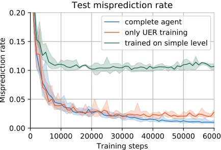
0 10000 20000 30000 40000 50000 60000 Training steps
0.00 0.05 0.10 0.15 0.20
Misprediction rate
Test misprediction rate complete agent only UER training trained on simple level
Figure 2: Transition misprediction rate on a randomly generated test set. The agent achieving the best performance uses count-based exploration, planning for exploration, UER and PER, and is followed by an agent that does not use planning for exploration and PER. In the last experiment (worst performance) the best agent is trained on a simple level with two boxes. Mean and standard deviation of 10 runs.
Each neural network has K2 inputs,3 followed by 4 fully connected layers of size 64, 128, 128, and 64, each with a leaky ReLU activation function h(x) = max(ax, x) with a = 0.01. Each layer computes a linear map of its inputs, followed by an element-wise application of the nonlinear activation function. The linear output layer hasK2 outputs, each representing
the change occurring in a pixel of the input neighbourhood following action execution.4 Unless otherwise stated, in our experiments we usedb= 100,NU ER= 80000,NP ER= 100,TP ER= 2,
α= 1, β= 50.
While training our agent, we measure its current prediction capability by testing it on a randomly generated test set of 100k local state–action pairs. In Fig.2we show examples of the resulting learning curve. In the plot, which compares our best algorithm with an agent learning only through UER, we observe that the former outperforms the latter after some time, as it keeps on learning and generalizing successfully, and after 50k time steps its misprediction rate is half. It can also be observed that an agent trained on a small level containing only two boxes cannot learn well and generalize, as there is not enough domain information for generalization.
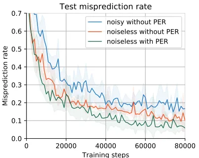
High-dimensional Noisy Observations. Here we present an experimental evaluation of model learning with noisy high-dimensional visual observations. The agent’s observations are a preprocessed version of the visual frame on the left in Figure1. We model noisy sensors by adding a Gaussian independent noise with varianceσ2 = 16/256 to each pixel. The resulting
noiseless and noisy observations are depicted in Figure3.
Figure 4 shows the transition misprediction rate when training on visual observations of the training level. PER is based onobserved transition mispredictions, which will occur at all times if observations are noisy, thereby making PER degenerate into online training. As this defies the purpose of UER, which is to decorrelate model updates, the agents trained from noisy
3 The smallestKfor which Sokoban satisfies theK-locality assumption is 5.
4Regarding learning the neighbourhood size,Kis increased by enlarging the input and output layers of each
Figure 3: Noiseless and noisy observations of the high-dimensional visual Sokoban environment on the left of Figure1.
0 20000 40000 60000 80000 Training steps
0.0 0.1 0.2 0.3 0.4 0.5 0.6 0.7
Misprediction rate
Test misprediction rate noisy without PER noiseless without PER noiseless with PER
Figure 4: Transition misprediction rate on a test set of 100k transitions, while training on the standard level. Both training and testing are based on the preprocessed visual observations in Figure3.
observations only use UER. In the plot we can observe the impact of noise by comparing the agents without PER, and at the same time appreciate the effect of PER in the noiseless case.
The higher dimensionality of observations clearly poses a challenge to the efficiency and quality of learning. This comes as no surprise, though, since the models we used are very simple neural networks. When dealing with high-dimensional observations, especially image-based, the transition model would greatly benefit from convolutional neural networks [12, 16,
5.2
Applying the Model to New Levels
In the previous section we have shown that the agent learns to predict a domain’s dynamics by training on one single level. Now we proceed to demonstrate how the gained knowledge can be immediately applied to new domain instances, with a different state space, initial state, and goal set, in contrast to typical model-based RL approaches. Note, however, that solving Sokoban instances efficiently is outside the scope of this work, which instead focuses on whether the learned model is accurate and general enough to eventually solve them. Results of clas-sical planners solving Sokoban can be found for example in the 2008 and 2011 issues of the International Planning Competition (IPC).
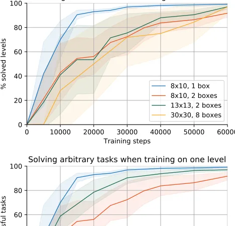
We train our agent on the fixed training level, in the low-dimensional noiseless case. During training, we make the agent solve new levels “offline”, with learning disabled. Its ability to solve levels is continuously assessed as it explores the training level and learns the game’s dynamics from it. Each test set contains Sokoban levels (randomly generated as in [30]) with the same board size and number of boxes. We let the agent try to solve all levels in a test set, given a goal test function that returns true if and only if the state is a goal state. The top plot in Fig.5
shows the percentage of solved test levels as a function of the number of training steps.
The specific search algorithm does not affect the results, as we are not considering the quality of the solution, nor the time to compute it. We use Breadth-First Search (BFS), except for the 30×30 levels where we use A* search with a simple domain-specific heuristic. Since we are only assessing whether a level is solved, it does not matter whether we are using BFS or A*. The only difference is that more nodes will be expanded using BFS, which takes prohibitively long in the 30×30 case. The initial state for planning is the current state, and the goal test function provides a termination condition. The plot shows that our agent can solve most levels after 60k training steps, with little dependence on their complexity and size. Levels with only one box are the only exception, as less training is required to solve them. The reason is that only relatively simple domain dynamics are involved there. On the other hand, dynamics of multiple-box interactions are more complex and encountered less often during training, and therefore are learned later.
The bottom plot in Fig. 5 shows the success rate when trying to achieve a different goal than solving the level. The new task consists in placing a box next to each target location, and is assigned to the agent through the goal test function. This task can often be completed without having learned dynamics that involve placing objects and agents on targets. These dynamics are the hardest to learn due to the lack of compositional entity-level information from the environment: a box on top of a target is perceived as one distinct entity that shares no evident property with the original box or target. For this reason, our agent is on average more successful in completing this new task in a given level, than in solving that level.
0 10000 20000 30000 40000 50000 60000 Training steps
0 20 40 60 80 100
% solved levels
Solving test levels when training on one level
8x10, 1 box 8x10, 2 boxes 13x13, 2 boxes 30x30, 8 boxes
0 10000 20000 30000 40000 50000 60000
Training steps 0
20 40 60 80 100
% successful tasks
Solving arbitrary tasks when training on one level
8x10, 1 box, solve level 8x10, 2 boxes, solve level 8x10, 2 boxes, other task
Figure 5: Percentage of tasks solved offline (learning disabled) by agents during training. There are 20 test levels for the 30×30 boards, and 200 for each of the other 3 configurations. Top: the task is always solving the level. Bottom: the test set with 8×10 levels with two boxes is also used with a modified task (green line). Mean and standard deviation for 6 agents are shown.
6
Related Work
In the recent years, there has been a growing interest in RL applied to high-dimensional domains, where deep network architectures have proven to be useful [16, 15,22,14]. However, state-of-the-art model-free deep RL models tend to be biased towards training experience, unable to generalize to similar tasks [10,21]. Moreover, in many complex or temporally extended tasks, some degree of planning is necessary, as short-term reactive decisions typical of model-free methods are not powerful enough.
higher-dimensional visual observations. The Interaction Network [3] and the Neural Physics Engine [4] learn models of intuitive physics that are more general than pixel-based prediction, but they rely on explicit object-level representations and hard-coded relations between entities. Another promising research direction is indicated by Value Iteration Networks [26] and the Pre-dictron [24], which implement end-to-end learning and planning, although their generalization and planning capability are still limited [11].
The focus of our work is to learn an environment model such that learning is efficient and the model generalizes well to new scenarios. To achieve this, we make a locality assumption on the domain’s dynamics, and we assume that any arbitrary goal can be assigned to the agent (no reward signal is involved). In [30] an environment model is also learned separately, but no particular assumption is made about the environment except for a fixed board size that is used throughout all experiments. Thus, the model learns general Sokoban dynamics only for a fixed, relatively small board size, and it needs about 109 training steps to do so (more than 4
orders of magnitude more than our approach). The agent (called I2A) also learns a policy from observing a reward signal, whereas we decouple learning from goal-oriented behaviour (and when planning to demonstrate the model effectiveness, we assume the goal is given from the start) and do not consider learning a policy. This would make the comparison unfair to our advantage, although I2A can exploit shaping rewards that constitute domain knowledge. The environment model proposed by Kansky et al. [11] efficiently learns the relationships between objects, thereby allowing causal reasoning and planning also in new scenarios. In contrast to our approach, the model relies on entity-level observations, and the problem is still framed as an RL problem, with a reward signal that is used for planning to test the model’s effectiveness.
Although more sparse and spread out in time, the literature on learning action models for automated planning is also rich. Many proposals in this area rely on prior domain knowledge such as examples of successful plans, or learn offline, after the training data has been gath-ered [29, 31, 19, 32, 6]. Among those which do not make such assumptions, e.g. [1, 20], the work by Mour˜ao et al. [17] is the most similar to ours. Their system learns implicit action mod-els from partial and noisy symbolic observations, then extracts symbolic rules and combines them into STRIPS-like action schemas. However, conditional effects are not supported, whereas our proposed method naturally learns them. A common characteristic of action model learning approaches is that they learn from logical descriptions of environment observations. Although such descriptions might be automatically generated from a low-dimensional input, this is not easy with high-dimensional observations. And even when the input is low-dimensional, it can-not generally be assumed to be entity-based: if a number of predicates are true forx(e.g. cell
xis a target and a box is onx), in the framework of our paper the agent will not be able to distinguish the different predicates (e.g. it will only observe that inxthere is abox-on-target entity, and the decoupling of box and target would have to be learned).
A different line of work deals with learning generalised policies for planning problems [8,
7
Conclusions and Future Work
We presented an approach that learns from raw visual observations an implicit transition model of planning domains. The learned dynamics can be applied to tree search to solve new instances of the training domain, given a goal. In contrast to action model learning in automated plan-ning, our approach does not rely on logical or entity-based observations of the environment. Compared to model learning methods in machine learning, it naturally generalizes to unseen instances, and in practice it learns more efficiently. Moreover, since goals are assigned to the agent explicitly, if the task is changed one simply needs to assign the new goal to the agent, instead of having it learn a new policy from an updated reward signal.
One main limitation of our approach is that the locality assumption imposes a restriction on the type of domains that can be used. Although many standard planning domains in which the STRIPS scope assumption holds [28] are in principle supported, there are domains – including both video games and real-world applications – in which this does not hold. In future work we want our method to rely on a weaker locality assumption. Furthermore, the learning algorithm does not produce explicit action schemas, and thus cannot be directly used with traditional off-the-shelf planners (e.g. FastDownward [9]). Future work also includes extending the method to handle stochastic environments and higher-dimensional visual representations.
References
[1] Amir, E. “Learning Partially Observable Deterministic Action Models”. In: JAIR 33 (2008), pages 349–402.
[2] Barto, A., Mirolli, M., and Baldassarre, G. “Novelty or Surprise?” In:Frontiers in Psy-chology 4 (2013).
[3] Battaglia, P., Pascanu, R., Lai, M., Rezende, D. J., et al. “Interaction networks for learning about objects, relations and physics”. In:NIPS. 2016, pages 4502–4510.
[4] Chang, M. B., Ullman, T., Torralba, A., and Tenenbaum, J. B. “A compositional object-based approach to learning physical dynamics”. In:ICLR. 2017.
[5] Chiappa, S., Racaniere, S., Wierstra, D., and Mohamed, S. “Recurrent environment sim-ulators”. In:ICLR. 2017.
[6] Cresswell, S. and Gregory, P. “Generalised Domain Model Acquisition from Action Traces”. In:ICAPS. 2011.
[7] Dor, D. and Zwick, U. “SOKOBAN and other motion planning problems”. In: Computa-tional Geometry 13.4 (1999), pages 215–228.
[8] Groshev, E., Tamar, A., Srivastava, S., and Abbeel, P. “Learning generalized reactive policies using deep neural networks”. In:arXiv preprint arXiv:1708.07280 (2017).
[9] Helmert, M. “The fast downward planning system”. In:JAIR26 (2006), pages 191–246.
[10] Jaderberg, M., Mnih, V., Czarnecki, W. M., Schaul, T., Leibo, J. Z., Silver, D., and Kavukcuoglu, K. “Reinforcement learning with unsupervised auxiliary tasks”. In:ICLR. 2017.
[12] Krizhevsky, A., Sutskever, I., and Hinton, G. E. “ImageNet Classification with Deep Convolutional Neural Networks”. In:NIPS. 2012, pages 1097–1105.
[13] Lai, T. L. and Robbins, H. “Asymptotically efficient adaptive allocation rules”. In: Ad-vances in applied mathematics 6.1 (1985), pages 4–22.
[14] Lillicrap, T., Hunt, J., Pritzel, A., Heess, N., Erez, T., Tassa, Y., Silver, D., and Wierstra, D. “Continuous control with deep reinforcement learning”. In:ICLR. 2016.
[15] Mnih, V., Badia, A. P., Mirza, M., Graves, A., Lillicrap, T., Harley, T., Silver, D., and Kavukcuoglu, K. “Asynchronous methods for deep reinforcement learning”. In: ICML. 2016, pages 1928–1937.
[16] Mnih, V., Kavukcuoglu, K., Silver, D., Rusu, A. A., Veness, J., Bellemare, M. G., Graves, A., Riedmiller, M., Fidjeland, A. K., Ostrovski, G., et al. “Human-level control through deep reinforcement learning”. In:Nature 518.7540 (2015), pages 529–533.
[17] Mour˜ao, K., Zettlemoyer, L., Petrick, R. P., and Steedman, M. “Learning STRIPS oper-ators from noisy and incomplete observations”. In:Twenty-Eighth Conference on Uncer-tainty in Artificial Intelligence (UAI2012)(2012), pages 614–623.
[18] Oh, J., Guo, X., Lee, H., Lewis, R., and Singh, S. “Action-Conditional Video Prediction using Deep Networks in Atari Games”. In:NIPS (2015), pages 2863–2871.
[19] Pasula, H. M., Zettlemoyer, L. S., and Kaelbling, L. P. “Learning Symbolic Models of Stochastic Domains”. In:JAIR29 (2007), pages 309–352.
[20] Rodrigues, C., G´erard, P., and Rouveirol, C. “Incremental learning of relational action models in noisy environments”. In:International Conference on Inductive Logic Program-ming (ILP). Springer. 2010, pages 206–213.
[21] Rusu, A. A., Rabinowitz, N. C., Desjardins, G., Soyer, H., Kirkpatrick, J., Kavukcuoglu, K., Pascanu, R., and Hadsell, R. “Progressive neural networks”. In: arXiv preprint arXiv:1606.04671 (2016).
[22] Schaul, T., Quan, J., Antonoglou, I., and Silver, D. “Prioritized Experience Replay”. In: ICLR. 2016.
[23] Silver, D., Huang, A., Maddison, C. J., Guez, A., Sifre, L., Van Den Driessche, G., Schrit-twieser, J., Antonoglou, I., Panneershelvam, V., Lanctot, M., et al. “Mastering the game of Go with deep neural networks and tree search”. In:Nature 529 (2016), pages 484–489.
[24] Silver, D., Hasselt, H. van, Hessel, M., Schaul, T., Guez, A., Harley, T., Dulac-Arnold, G., Reichert, D., Rabinowitz, N., Barreto, A., et al. “The predictron: End-to-end learning and planning”. In:arXiv preprint arXiv:1612.08810 (2016).
[25] Strehl, A. L. and Littman, M. L. “An analysis of model-based interval estimation for Markov decision processes”. In: Journal of Computer and System Sciences 74.8 (2008), pages 1309–1331.
[26] Tamar, A., Wu, Y., Thomas, G., Levine, S., and Abbeel, P. “Value Iteration Networks”. In:NIPS (2016), pages 2154–2162.
[27] Toyer, S., Trevizan, F., Thiebaux, S., and Xie, L. “Action Schema Networks: Generalised Policies with Deep Learning”. In:arXiv preprint arXiv:1709.04271 (2017).
[29] Wang, X. “Learning by observation and practice: An incremental approach for planning operator acquisition”. In:ICML(1995).
[30] Weber, T., Racani`ere, S., Reichert, D. P., Buesing, L., Guez, A., Rezende, D. J., Badia, A. P., Vinyals, O., Heess, N., Li, Y., et al. “Imagination-Augmented Agents for Deep Reinforcement Learning”. In:NIPS. 2017.
[31] Yang, Q., Wu, K., and Jiang, Y. “Learning action models from plan examples using weighted MAX-SAT”. In:Artificial Intelligence 171.2-3 (2007), pages 107–143.