Optimal Control of Switched Systems by a Modified
Pseudo Spectral Method
HAMID REZA TABRIZIDOOZ,MARZIEH POURBABAEE AND MEHRNOOSH HEDAYATI
Department of Applied Mathematics, Faculty of Mathematical Sciences, University of Kashan, Kashan 87317–53153, Iran
ARTICLE INFO ABSTRACT
Article History:
Received 18 January 2016 Accepted 16 April 2016 Published online 5 April 2017 Academic Editor: IVAN GUTMAN
In the present paper, we develop a modified pseudo spectral scheme for solving an optimal control problem which is governed by a switched dynamical system. Many real–world processes such as chemical processes, automotive systems and manufacturing processes can be modeled as such systems. For this purpose, we replace the problem with an alternative optimal control problem in which the switching times appear as unknown parameters. Using the Legendre–Gauss–Lobatto quadrature and the corresponding differentiation matrix, the alternative problem is discretized to a nonlinear programming problem. At last, we examine three examples in order to illustrate the efficiency of the proposed method.
© 2017 University of Kashan Press. All rights reserved Keywords:
Optimal control Switched systems
Legendre pseudo spectral method
1.
I
NTRODUCTIONIt is well known that pseudospectral (PS) methods are powerful methods for the numerical solution of differential equations. In fact, they arose from spectral methods which were traditionally used to solve fluid dynamics problems [1, 2]. They can often achieve ten digits of accuracy where a finite difference scheme or a finite element method would get two or three [3]. The key point in PS methods is that they avoid the poor behavior of the classical polynomial interpolation methods by removing the restriction to equally spaced interpolation points.
The variational method of optimal control theory, which typically consists of the calculus of variations and Pontryagin’s methods, can be used to derive a set of necessary conditions that must be satisfied by an optimal control law and its associated state–control equations [4, 5]. These necessary conditions of optimality lead to a generally nonlinear
Corresponding Author: (Email address: [email protected]) DOI: 10.22052/ijmc.2017.44718
Iranian Journal of Mathematical Chemistry
two–point boundary value problem that must be solved to determine the explicit expression for the optimal control. Except in some special cases, the solution of this two–point boundary value problem is difficult and not practical to obtain.
Various alternative computational techniques for optimal control problems have been developed in the literature. The techniques are basically of three types: parameterization on both state and control [6, 7, 8], parameterization on control only [9, 10] and nonparameterization [11, 12, 13]. As a technique of the first type, PS methods can be interpreted as direct transcription methods for discretizing a continuous optimal control problem into a nonlinear programming (NLP) problem [14, 15, 16, 17, 18, 19]. The resulting NLP problem can be solved numerically by the well developed algorithms [20, 21].
Although PS methods enjoy many nice properties, but their use in solving problems with nonsmooth solutions or problems with switches may cause major difficulties. The reason lies in the famous Gibbs phenomenon which happens when a nonsmooth function is approximated by means of a finite number of smooth functions [2]. In [22], the authors developed the method of PS knotting in order to address this issue. In fact, they introduced the concepts of hard and soft knots to eliminate the mentioned difficulties.
The switched systems are a particular class of hybrid systems. The hybrid systems arise in varied contexts in chemical processes, automotive engine control, traffic control, and manufacturing processes, etc. The abundance of hybrid phenomena in many engineering systems in general, and in the chemical process industries in particular has fostered a large and growing body of research work in this area [23, 24, 25, 26, 27, 28, 29, 30]. In [31], the authors discussed important hybrid aspects of chemical processing plants. Recently, optimal control of switched systems arising in fermentation processes has been studied in [32]. A hybrid system consists of several subsystems and a switching law, where the switching law is determined by a switching sequence and a set of switching times. At each time instant, only one subsystem is active. A hybrid system can be described by a differential inclusion of the form
( , (), ( )): {1,2, , }
, )(t f t x t u t v M
x v (1)
where t[t0,tf], ( )∈ ℝ , ( )∈ ℝ and for eachv{1,2,,M}, :ℝ×ℝ ×ℝ → ℝ , is continuously differentiable with respect to its arguments. A switching law for system (1) is defined as =((t0,i0),(t1,i1),,(tK1,iK1)), where 1K <,
f K t
t t
method which is based on parameterization of the switching instants is proposed for this kind of optimal control problems.
In this paper, we investigate a modified Legendre PS scheme in order to explore accurate and efficient solutions of optimal control problems for switched systems. Here, we consider the optimal control problems in which a prespecified sequence of active subsystems is given. In order to explore numerical solutions of such problems, we need to seek the solutions of both the optimal switching instants and the optimal piecewise input. The rest of this paper is organized as follows. The problem statement is given in Section 2. In Section 3, we describe the preliminaries for subsequent development. The present method is proposed in Section 4. Then, three examples are provided in Section 5 to illustrate the efficiency of the proposed method. Conclusions are presented in Section 6.
2.
P
ROBLEMS
TATEMENTWe consider switched systems defined on the fixed time interval [t0,tf] with K1
switches, consisting of the subsystems
) 2 ( ,
, 1,2, = ), , [ )), ( ), ( ( = )
(t f x t u t t t 1 t k K
x k k k
with initial conditions
) 3 ( ,
= ) (t0 x0 x
where ( ) = ( ( ), … , ( ))∈ ℝ is the state function and ( ) = ( ( ), … , ( ))∈ ℝ is the corresponding control function. Also, :ℝ ×ℝ → ℝ , k =1,2,,K, are given functions. We assume that the switching sequence is preassigned, such that
) 4 ( ,
=
1 1
0 t tK tK tf
t
where the switching times t1,,tK1 are decision variables. Our objective is to find a piecewise continuous function u(t) and switching instants t1,,tK1 subject to the condition (4) for the switched system (2) and (3) such that the cost functional
) 5 ( ))
( ), ( ( ))
( ( =
0
dt t u t x g t
x
J tf
t f
3.
P
RELIMINARIESLet 0 <1<<N be the Legendre–Gauss–Lobatto (LGL) nodes where 0 =1, N =1 and 1,,N1 are the roots of PN(). Here PN() is the derivative of the N –th order
Legendre polynomial PN(). In other words, the LGL points 0,1,,N are the N1
roots of (12)PN(). The reader is referred to [1, 34] for details.
Let h(t) be a continuous real function which is defined on [1,1]. The Lagrange interpolating polynomial of degree N interpolates the function h(t) at the points
N
0, 1,, , as
). ( ) ( )
(
0 =
j j
N
j
L h
h
(6)Here for j=0,1,,N, Lj() denotes the Lagrange polynomial of degree N
corresponding to the point j, defined by
. =
) (
, 0
= j i i N
j i i j
L
Note that the Lagrange polynomials satisfy in the Kronecker property
. 0,
= 1, = ) (
i j
i j Lj i
In order to approximate the derivative of h(t) at the points i, i=0,1,,N, the interpolation formula (6) is differentiated yielding
), ( )
(
0 =
j ij N
j
i d h
h
(7)where dij =Lj(i). The (N1)(N1) matrix D=[dij] is the so–called derivative
matrix. According to [1]
.
0,
= = ,
4 1) (
0 = = ,
4 1) (
, 1 ) (
) (
=
otherwise N j i N
N
j i N
N
j i P
P
d
j i j N
i N
ij
), ( ) ( 0 = 1
1 j j
N
j
h w d
h
(8)
where wj, j=0,1,,N, are the LGL weights, corresponding to the LGL points j,
N
j=0,1,, , given by
( )
, =0,1, , .1 1) (
2
= 2 j N
P N N w j N j
4.
P
ROPOSEDM
ETHODWe suppose that in the problem stated in the Eqs. (2)–(5), the switching sequence is preassigned and t1,,tK1 are the corresponding unknown switching times for which the condition (4) holds.
We denote the restriction of vector functions x(t) and u(t) to the k–th subinterval )
,
[tk1 tk by xk(t)
and uk(t)
, respectively. According to these notations, the dynamic
subsystems in Eq. (2) are expressed as
x (t)= f (x (t),u (t)), tk 1 t<tk, k =1, ,K, k k k k
(9)
. , 2, = ), ( lim = ) ( 1 1
1 x t k K
t x k k t t k k
(10)
Note that in Eq. (10), the continuity constraints are added in order to guarantee the continuity of state functions. Accordingly, the cost functional (5) reformulated as
, )) ( ), ( ( )) ( ( = 1 1 = dt t u t x g t x
J tk k k
k t K k f K
(11)
and the initial conditions (3) restated as
. = ) (0 0 1
x t
x (12)
To apply the approximations described in the previous section, we must transfer each subinterval to the interval [1,1]. For this purpose, we use the transformation formula
1 1 ) ( 2 = k k k k t t t t t
in the k–th subinterval [tk1,tk). In this respect, the problem is restated
in the following alternative form:
x t t g x u d
J k k k k
K k K )) ( ), ( ( 2 (1)) ( = min 1 1 1 1 =
(13)
( ( ), ( )), =1, , ,
2 = ) ( .
.tx t t 1 f x u k K
s k k k k k k
(14)
. = 1) ( 0 1 x
x (16)
The alternative problem (13)–(16) provides us with some advantage, namely that it no longer has varying switching instants. In fact, the switching instants are considered as parameters in the alternative problem.
It has to be noted that for k=1,,K, the components of vector functions k() x
and k()
u are smooth on [1,1] and then can be expanded in terms of Lagrange basis functions according to Eq. (6). Therefore, using the formula (8), the performance index J in Eq. (13) is approximated as
, ) , ( 2 ) ( ( ) ( ) 0 = 1 =1 ) ( j k j k j N j k k K k K
N g X U w
t t X
J
(17)
where X(jk) and U(jk) are vectors in ℝ and ℝ , respectively, and defined by
. , 1, = , , 0,1, = ), ( = ), ( = ( ) ) ( K k N j u U x X j k k j j k k
j
Also, using the formula (7), the alternative dynamical systems (14) are approximated by
, , 1, = 0, = 2 ) ( 1 ) ( K k F t t X
D k k k k
(18)
where X(k) and F(k) are (N1)n matrices, respectively, defined by
. ) , ( ) , ( ) , ( = , = ) ( ) ( ) ( 1 ) ( 1 ) ( 0 ) ( 0 ) ( ) ( ) ( 1 ) ( 0 ) ( k N k N k k k k k k k k k N k k k U X f U X f U X f F X X X X
Furthermore, the continuity constraints (15) and the initial conditions (16), respectively, are stated as , , 2, = 0, = 1) ( ) (
0 X k K
X k Nk
(19)
and
. = 0 (1) 0 x
X (20)
We also assume that no two endpoints of subintervals coincide. Then, for a small given 0
>
, we add the extra constraints
. , 1, = , >
1 k K
t
tk k (21) In summary, the alternative optimal control (13)–(16) is discretized to the following NLP
problem: Find vectors X(jk),
) (k j
U , j=0,1,,N, k=1,,K and the parameters tk, 1
, 1,
= K
The relations between the solutions of obtained NLP problem and the solutions of alternative problem (13)–(16) are given by
, , 1, = ), ( ) ( ( ) 0 = ) ( K k L X x j k j N j k
and . , 1, = ), ( ) ( ( ) 0 = ) ( K k L U u jk jN j k
5.
I
LLUSTRATIVEE
XAMPLESIn this section, we consider three examples to illustrate the efficiency of proposed method. Here, we consider the numerical examples given in [33]. According to the present method, each example in modeled using the mathematical software package Maple 17 and the resulting NLP problems are solved by the command NLPSolve.
Example 1. Consider a switched system consisting of nonlinear subsystems
. ) ( cos ) ( ) ( = ) ( ) ( sin ) ( ) ( = ) ( : 3 , ) ( cos ) ( ) ( = ) ( ) ( sin ) ( ) ( = ) ( : 2 , ) ( cos ) ( ) ( = ) ( ) ( sin ) ( ) ( = ) ( : 1 2 2 2 1 1 1 1 1 2 2 2 1 2 2 2 1 1 1 t x t u t x t x t x t u t x t x subsystem t x t u t x t x t x t u t x t x subsystem t x t u t x t x t x t u t x t x subsystem
Assume that t0 =0, tf =3 and the system switches at t=t1 from subsystem 1 to 2 and at 2
=t
t from subsystem 2 to 3 (0t1t2 3). The initial conditions are x1(0)=2 and
3 = (0) 2
x . We want to find optimal switching instants t1, t2 and an optimal input u(t) such that the cost functional
dt t u t x t x x x
J [( ( ) 1) ( ( ) 1) ( )]
2 1 1) (3) ( 2 1 1) (3) ( 2 1
= 3 1 2 2 2 2
0 2 2
2
1
is minimized.
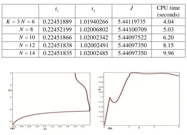
In Table 1, we listed the results of optimal switching instants t1, t2 and optimal cost
Table 1. The results of optimal switching instants t1, t2 and optimal cost J obtained by the present method with K =3 and different values of N , for Example 1.
1
t t2 J CPU time
(seconds)
6 = 3 = N
K 0.22451889 1.01940266 5.44119735 4.04
N =8 0.22452199 1.02006802 5.44100709 5.03
N =10 0.22451866 1.02002342 5.44097522 6.20
N =12 0.22451838 1.02002491 5.44097350 8.15
N =14 0.22451835 1.02002485 5.44097350 9.96
Figure 1: The graphs of (a) state trajectory and (b) optimal control obtained by the present method with K =3 and N =9, for Example 1.
Example 2. Consider a switched system consisting
). ( 1 2 ) ( ) ( 0 1 3 4 = ) ( ) ( : 2 ), ( 1 1 ) ( ) ( 4 . 3 8 . 0 2 . 1 6 . 0 ) ( ) ( : 1 2 1 2 1 2 1 2 1 t u t x t x t x t x subsystem t u t x t x t x t x subsystem
Assume that t0 =0, tf =2 and the system switches once at t =t1 (0t12) from subsystem 1 to 2. The initial conditions are x1(0)=0 and x2(0)=2. We want to find an
optimal switching instant t1 and an optimal input u(t) such that the cost functional
dt t u t x x x
J [( ( ) 2) ( )]
2 1 2) (2) ( 2 1 4) (2) ( 2 1
= 2 2
2 2 0 2 2 2
1
We applied the proposed method to solve this example. In Table 2, we reported the results of t1 and J obtained by the present method with K =2 and different values of N . Also in Figure 2, we plot the graphs of optimal control and the corresponding state trajectory with K =2 and N =9.
Table 2.The results of optimal switching instant t1 and optimal cost J obtained by the present method with K =2 and different values of N , for Example 2.
t1 J CPU time
(seconds)
6 = 2 = N
K 0.19007133 9.78402619 2.62
N =8 0.18967215 9.76657993 3.04
N =10 0.18967109 9.76654884 3.46
N =12 0.18967110 9.76654882 4.42
N =14 0.18967107 9.76654882 5.60
Figure 2: The graphs of (a) state trajectory and (b) optimal control obtained by the present method with K =2 and N =9, for Example 2.
Example 3. Consider a switched system with internally forced switching only consisting of
). ( 1 1
) (
) (
0.5 0.866
0.866 0.5
= ) (
) ( : 2
), ( 1 1
) (
) (
1 0
0 1.5
) (
) ( : 1
2 1
2 1
2 1
2 1
t u t
x t x
t x
t x subsystem
t u t
x t x
t x
t x subsystem
Assume that t0 =0, tf =2 and the system state starts at x1(0)=1, x2(0)=1, following subsystem 1 (subsystem 1 is active for c(x1(t),x2(t))= x1(t)x2(t)70 and
subsystem 2 is active for c(x1(t),x2(t))0). Assume that upon intersecting the hyper
surface c(x1,x2)=0, the system switches from subsystem 1 to 2. Also, assume there is only
one switching which takes place at time t1 (0t12). We want to find an optimal input
) (t
u such that the cost functional
dt t u x
x
J ( )
2 1 6) (2) ( 2 1 10) (2) ( 2 1
= 2 2
0 2 2
2
1
is minimized.
Note that we have not considered state constraints in the subsystems of our problem modeled by Eqs. (2)–(5). For this reason, we state our technique in order to approximate state constraints. By setting K =2, according to the proposed method, we have two sets of state functions values: X(1)j , j=0,1,,N, are the values of state functions in subsystem 1,
and X(2)j , j=0,1,,N, are the values of state functions in subsystem 2. According to this,
we obtain the constraints c(X(1)j )0, j=0,1,,N, in subsystem 1, and ( ) 0
(2) c Xj ,
N
j=0,1,, , in subsystem 2. These new inequality constraints must be added to Eqs. (18)–(21).
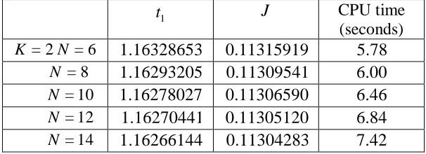
In Table 3, we listed the results of t1 and J obtained by the present method with
2 =
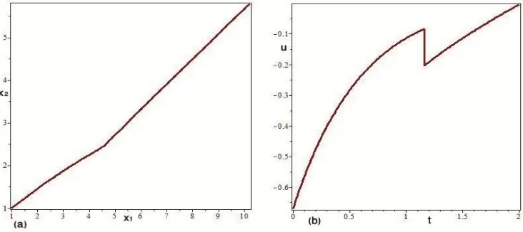
K and different values of N . Also in Figure 3, we plot the graphs of optimal control and the corresponding state trajectory with K =2 and N =9.
Table 3. The results of optimal switching instant t1 and optimal cost J obtained by the present method with K =2 and different values of N , for Example 3.
1
t J CPU time
(seconds)
6 = 2 = N
K 1.16328653 0.11315919 5.78
N =8 1.16293205 0.11309541 6.00
N =10 1.16278027 0.11306590 6.46
N =12 1.16270441 0.11305120 6.84
Figure 3: The graphs of (a) state trajectory and (b) optimal control obtained by the present method with K =2 and N =9, for Example 3.
6.
C
ONCLUSIONIn this paper, we have considered a class of optimal control problems governed by switched systems. Such systems arise in varied contexts in chemical processes, automotive engine control, traffic control, and manufacturing processes, etc. We have proposed a modified Legendre pseudospectral scheme in order to explore accurate solutions. For this purpose, we have restated the problem in form of an alternative problem in which the switching instants are considered as parameters. Then, we can solve the obtained NLP problem using existing subroutines. Three numerical examples considered in order to show the validity and applicability of the proposed method.
R
EFERENCES1. C. Canuto, M. Y. Hussaini, A. Quarteroni and T. A. Zang, Spectral Methods: Fundamentals in Single Domains, Springer–Verlag, Berlin, 2006.
2. B. Fornberg, A Practical Guide to Pseudospectral Methods, Cambridge University Press, 1996.
3. L. N. Trefethen, Spectral Methods in MATLAB, SIAM, Philadelphia, 2000.
4. D. E. Kirk, Optimal Control Theory, Prentice–Hall, Englewood Cliffs, New Jersey, 1970.
5. L. S. Pontryagin, V. Boltyanskii, R. Gamkrelidze and E. Mischenko, The Mathematical Theory of Optimal Processes, Interscience Publishers, New York, 1962.
7. J. Vlassenbroeck, A Chebyshev polynomial method for optimal control with state constraint, Automatica24 (1988) 499–506.
8. J. Vlassenbroeck and R. Van Doreen, A Chebyshev technique for solving nonlinear optimal control problems, IEEE Trans. Automat. Control 33 (1988) 333–340. 9. C. J. Goh and K. L. Teo, Control parametrization: a unified approach to optimal
control problems with general constraint, Automatica24 (1988) 3–18.
10.O. Rosen and R. Luus, Evaluation of gradients for piecewise constraint optimal control, Computers and Chemical Engineering15 (1991) 273–281.
11.W. W. Hager, Multiplier methods for nonlinear optimal control, SIAM J. Numer. Anal. 27 (1990) 1061–1080.
12.D. H. Jacobson and M. M. Lele, A Transformation technique for optimal control problems with a state variable inequality constraints, IEEE Trans. Automat. Control AC–14 (1969) 457–464.
13.E. Polak, T. H. Yang and D. Q. Mayne, A method of centers based on barrier function methods for solving optimal control problems with continuum state and control constraints, SIAM J. Control Optim. 31 (1993) 159–179.
14.G. N. Elnagar, M. A. Kazemi and M. Razzaghi, The pseudospectral Legendre method for discretizing optimal control problems, IEEE Trans. Automat. Control 40 (1995) 1793–1796.
15.G. N. Elnagar and M. A. Kazemi, Pseudospectral Chebyshev optimal control of constrained nonlinear dynamical systems, Comput. Optim. Appl. 11 (1998) 195– 217.
16.F. Fahroo and I. M. Ross, Costate estimation by a Legendre pseudospectral method, J. Guid. Control Dyn.24 (2001) 270–277.
17.G. T. Huntington, D. A. Benson and A. V. Rao, Post–optimality evaluation and analysis of a formation flying problem via a Gauss pseudospectral method, 2005, AAS paper no. 05–339.
18.Q. Gong, W. Kang and I. M. Ross, A pseudospectral method for the optimal control of constrained feedback linearizable systems, IEEE Trans. Automat. Control 51
(2006) 1115–1129.
19.M. Shamsi, A modified pseudospectral scheme for accurate solution of Bang–Bang optimal control problems, Optimal Control Appl. Methods32 (2011) 668–680. 20.R. Fletcher, Practical Methods of Optimization, John Wiely, Chichester, 1987. 21.J. Nocedal and S. J. Wright, Numerical Optimization, Springer Series in Operations
Research, Springer, New York, 1999.
23.I. E. Grossmann, S. A. Van Den Heever and I. Harjukoski, Discrete optimization methods and their role in the integration of planning and scheduling, AIChE Symposium Series98 (2002) 150–168.
24.N. H. El–Farra, P. Mhaskar and P. D. Christofides, Feedback control of switched nonlinear systems using multiple Lyapunov functions, in Proceedings of American Control Conference, pages 3496–3502, Arlington, VA, 2001.
25.R. A. Decarlo, M. S. Branicky, S. Petterson and B. Lennartson, Perspectives and results on the stability and stabilizability of hybrid systems, Proceedings of the IEEE88 (2000) 1069–1082.
26.A. Bemporad and M. Morari, Control of systems integrating logic, dynamics and constraints, Automatica35 (1999) 407–427.
27.B. Hu, X. Xu, P. J. Antsaklis and A. N. Michel, Robust stabilizing control law for a class of second–order switched systems, Systems Control Lett. 38 (1999) 197–207. 28.N. H. El–Farra, P. Mhaskar and P. D. Christofides, Output feedback control of
switched nonlinear systems using multiple Lyapunov functions, Systems Control Lett.54 (2005) 1163–1182.
29.R. Ghosh and C. Tomlin, Symbolic reachable set computation of piecewise affine hybrid automata and its application to biological modelling: Delta–Notch protein signalling, Syst. Biol. 1 (2004) 170–183.
30.P. G. Howlett, P. J. Pudney and X. Vu, Local energy minimization in optimal train control, Automatica 45 (2009) 2692–2698.
31.S. Engell, S. Kowalewski, C. Schulz and O. Stursberg, Continuous–discrete interactions in chemical processing plants, Proceedings of the IEEE 88 (2000) 1050–1068.
32.C. Liu and Z. Gong, Optimal Control of Switched Systems Arising in Fermentation Processes, Springer–Verlag, Berlin Heidelberg, 2014.
33.X. Xu and P.J. Antsaklis, Optimal control of switched systems based on parameterization of the switching instants, IEEE Trans. Automat. control49 (2004) 2–16.