A policy iteration algorithm for nonzero-sum stochastic impulse games

B. Bouchard, J.-F. Chassagneux, F. Delarue, E. Gobet and J. Lelong, Editors

A POLICY ITERATION ALGORITHM FOR NONZERO-SUM STOCHASTIC

IMPULSE GAMES

Ren´

e A¨ıd

, Francisco Bernal

, Mohamed Mnif

, Diego Zabaljauregui

and Jorge P. Zubelli

Abstract. This work presents a novel policy iteration algorithm to tackle nonzero-sum stochastic impulse games arising naturally in many applications. Despite the obvious impact of solving such problems, there are no suitable numerical methods available, to the best of our knowledge. Our method relies on the recently introduced characterisation of the value functions and Nash equilibrium via a system of quasi-variational inequalities. While our algorithm is heuristic and we do not provide a convergence analysis, numerical tests show that it performs convincingly in a wide range of situations, including the only analytically solvable example available in the literature at the time of writing.

R´esum´e. Ce travail pr´esente un nouvel algorithme d’it´eration sur les politiques pour approximer num´eriquement les fonctions valeurs d’un probl`eme de jeux impulsionnels stochastiques `a somme non nulle. Ces probl`emes apparaissent naturellement de nombreuses situations ´economiques de concur-rence entre acteurs. A notre connaissance, malgr´e l’int´erˆet pratique de solutions num´eriques `a de tels probl`emes, il n’existe pas d’algorithmes appropri´ees. Notre m´ethode repose sur la caract´erisation r´ecemment introduite des fonctions valeur et de l’´equilibre de Nash par un syst`eme d’in´egalit´es quasi-variationnelles. Bien que l’on ne fournisse pas d’analyse de convergence, des tests num´eriques effectu´es dans un large ´eventail de situations illustrent l’efficacit´e de notre algorithme. Enfin, nous montrons qu’il converge `a la solution dans le seul cas connu de solution analytique.

Keywords: stochastic impulse game, nonzero-sum game, Nash equilibrium, policy iteration, Howard’s algo-rithm, quasi-variational inequality.

Introduction

Stochastic impulse games (SIGs) are at the intersection between differential game theory and stochastic impulse control. In the case of one sole player, they reduce to stochastic impulse optimisation problems where an agent seeks to control an underlying (or state variable)—otherwise governed by a stochastic differential equation—in order to maximize the expected value of some target functional. One way in which she can influence the underlying is this: whenever it leaves acontinuation region (i.e. at her intervention times), she suddenly shifts it back somewhere into the region (by providing animpulse). Together, the continuation region

1 _{Universit´e Paris Dauphine, PSL Research University, LEDA.}

2 _{CMAP, Ecole Polytechnique, and Finance for Energy Market Research Centre (FiME).}

3 _{University of Tunis El Manar, ENIT-LAMSIN.}

4 _{Corresponding Author. Department of Statistics, London School of Economics and Political Science.} E-mail: [email protected]

5 _IMPA.

c

EDP Sciences, SMAI 2019

This is an Open Access article distributed under the terms of the Creative Commons Attribution License (http://creativecommons.org/licenses/by/4.0), which permits unrestricted use, distribution, and reproduction in any medium, provided the original work is properly cited.

and impulses define what we will call a strategy. Thus, the control-theoretical problem typically boils down to determining an optimal strategy as a function of the current value of the underlying. The purpose of the analysis is to apply that optimal strategy to any specific realization of the underlying. When such a strategy is followed, the expected value of the target functional—the largest possible—is called thevalue function. This problem is a classical one and it is well understood by now [10]. In particular, a rigorous framework has been put in place—combining Howard’s algorithm [3–5, 9] with viscosity-capturing finite difference schemes—which allows for robust numerical approximations [7, 8, 10].

A natural extension are two-player SIGs. In such games, two players seek to control the underlying with different, and often opposed, aims. Let us give two concrete examples, due to [1].

• Two central banks competing to influence the exchange rate between their respective currencies, both seeking to devalue their own one. In this application, the exchange rate is modelled as a stochastic process, and either central bank intervenes when it deems its currency too strong. Each bank’s strategy is made up of the ensuing devaluation and the threshold exchange rate triggering it. Both quantities are to be optimally determined in advance, by solving the game.

• A wholesale producer of energy and a big client of hers who resells it. Due to the high consumption of the client, both players are capable of affecting the wholesale price of energy, with naturally opposed targets (a high price versus a low one, respectively). Each player incurs costs when modifying the price while possibly benefiting from state compensation upon adverse price movements led by the opponent. In order to avoid superfluous costs, both players need a strategy, based on the current wholesale price, determining the optimal triggering threshold and the extent of the price shift.

Contrary to one-player SIGs, the value functions in two-player SIGs (one for each player) cannot be naively defined by maximisation. Instead, optimality can naturally be characterized via the notion ofNash equilibrium: intuitively, the pair of value functions displays the best expected outcome in the sense that if a player changes her strategy while her opponent does not, then the former can only be worse off. A pair of strategies at which these values are attained is then called a Nash equilibrium. Because of this, two-player SIGs are distinctly different (and more complex) from one-player SIGs, and the theoretical/numerical frameworks for the latter are not suitable for the former. This is further accentuated in the so-callednonzero-sum SIGs (NZSSIGs), roughly meaning that the losses (resp. gains) undergone by one player may not exactly translate into gains (resp. losses) for the opponent. (For instance, the previously described examples are best modelled under this very flexible framework.) NZSSIGs are in contraposition with the simpler and more particularzero-sumSIGs, in which both value functions add up to zero—effectively reducing the problem to finding one. (This allows for more natural extensions of the theoretical and numerical tools of the one-player case [2, 6].)

Due to the greater complication involved in the analysis, NZSSIGs are much underdeveloped. Very recently, a breakthrough has been achieved in [1], where the value functions and a Nash equilibrium of a very general class of NZSSIGs (assuming they exist and possess some regularity) have been characterized via a system of quasi-variational inequalities (QVIs). Besides the theoretical interest of this link by itself, it opens up the possibility of finding approximations to the value functions by numerically solving that system.

even when an analytical solution is available, its computation in practice may involve parameters which require solving complex nonlinear systems of equations—thus stressing the convenience of numerical approximations.

Let us outline the organization of the rest of the paper. We start in Section 2 by properly setting up NZSSIGs and recalling the main result of [1], namely, the Verification Theorem with the corresponding system of QVIs. For the sake of illustration, the concrete application of competition in energy markets is presented according to this framework. In Section 3, we briefly review the state-of-the-art numerics for one-player SIGs, with an emphasis on Howard’s algorithm, which will later become a pivotal ingredient of our own numerical method for NZSSIGs. The latter is motivated, listed, and discussed in Section 4. Section 5 presents numerical evidence supporting it, in the light of which we draw some conclusions in Section 6.

1.

The theoretical model

1.1.

Two-player nonzero-sum stochastic impulse games

In this section we introduce a general class of two-player NZSSIG, to which our numerical algorithm is applicable. For the sake of briefness and pertinence, we will skip some of the most technical matters of the rigorous construction of the model. We refer the interested reader to [1] for more details and a more general modelling framework.

Let (Ω,F,(Ft)t≥0,P) be a filtered probability space under the usual conditions, that supports a standard one-dimensional Brownian motion W = (Wt). For eachx ∈ R we consider a process X (the state variable) starting atx,

Xt=x+ Z t

0

µ(Xs)ds+ Z t

0

σ(Xs)dWs+ X

k: τ1

k≤t

δ_k1+ X

k: τ2

k≤t

δ_k2, (1)

where:

(i) µ, σ:_R→_Rare Lipschitz continuous. (ii) ui _:={(τi

k, δki)}∞k=1 (i= 1,2) is thecontrol of player i, which consists of a sequence of stopping timesτki (the k-th intervention time of player i) and F_τi

k-measurable random variablesδ

i

k (the k-th intervention impulse of playeri).

In words, when none of the players intervenes the state variable behaves as an Itˆo diffusion. The players can at any time decide to shift this process by applying a certain impulse. The specific type of interventions are determined by(threshold-type) strategies, which means that each player acts only when the state variable exits a given region ofR. More specifically, the control of playeriis defined in terms of a strategyϕi:= (Ci, ξi),where

Ci⊆Ris an open set (the continuation region) andξi:Cic→Ris a continuous function.1 Playeri intervenes if X exits Ci—i.e., if for some t ≥0 and ω ∈Ω it holdsXt(w)∈ C/ i—by applying an impulse ξi(Xt(w)). We decree that the game never stops and if both players want to intervene at the same time, then player 1 has the priority. The latter assumption is a matter of convention and not very restrictive.2

Henceforth, we write _Ex to denote the conditional expectation given X0− = x, and define the objective

function for playerigiven the strategies (ϕ1, ϕ2) and the starting pointxofX as

Ji(x;ϕ1, ϕ2) :=Ex "

Z ∞

0

e−ρis_f

i(Xs)ds+

∞

X

k=1

e−ρiτki_φ

i X(τi k)−, δ

i k + ∞ X k=1

e−ρiτkjψ_i X

(τ_kj)−, δ

j k

#

, (2)

withi, j∈ {1,2}, j6=i; where:

(i) ρi>0 is the subjective discount rateof playeri.

1_{For anyA⊆}

R,Acdenotes the complement ofAinR.

2_{Under the assumptions of the Verification Theorem 1.2.1, the value of the game and the Nash equilibrium found would not}

(ii) fi:R→Ris a continuous function giving therunning payoff of playeri.

(iii) φi :R2→R(resp. ψi:R2→R) is a continuous function giving thecost of intervention (resp. gain due to the opponent’s intervention) for playeri.

In addition, we will only consider pairs of strategies (ϕ1, ϕ2) such that the previous expectations are well defined for all x∈R, and we refer to these pairs as admissible (see [1] for more details).3 Note for example that, for payoffs with polynomial growth, the ‘no intervention strategies’φ1=φ2= (R,∅) are always admissible. In this context, we say that the players behave optimally if their strategies form a Nash equilibrium. We recall that (ϕ∗1, ϕ∗2) is aNash equilibrium if it is an (admissible) pair of strategies such that, for all (ϕ1, ϕ2),

J1(x;ϕ∗₁, ϕ∗₂)≥J1(x;ϕ1, ϕ∗₂) and J2(x;ϕ∗₁, ϕ∗₂)≥J2(x;ϕ∗₁, ϕ2),

i.e., if player i changes strategy while player j does not, then on average player i will be worse off, and vice versa. If a Nash equilibrium (ϕ∗₁, ϕ∗₂) exists, we define thevalue function for playeriwhen using the strategies (ϕ∗1, ϕ∗2) by

Vi(x) :=Ji(x;ϕ1∗, ϕ∗2), i= 1,2. (3)

Our aim is to compute (V1, V2) for some Nash equilibrium, and more importantly, to retrieve from these values the equilibrium itself.

1.2.

The system of quasi-variational inequalities

In order to establish a system of QVIs for (V1, V2) we need to define one last ingredient, known as the intervention operators, which will display the effect of each player’s intervention on the value functions. For any two arbitrary functions ˜V1,V˜2:R→R,i, j∈ {1,2}, i6=j, andx∈R, theloss operator of playeriis given by

MiV˜i(x) := sup δ∈R

{V˜i(x+δ) +φi(x, δ)}. (4)

If ˜Vi =Vi this operator gives the recomputed present value ofi due to the cost of her own intervention. If for each x∈ _R there exists a uniqueδj_{(x) = δ}j

˜ Vj

(x) that realizes the supremum in (4) , we also define the gain

operator of playerias

HiV˜i(x) := ˜Vi(x+δj(x)) +ψi(x, δj(x)). (5)

If ˜Vi = Vi this operator gives the recomputed present value of player i due to her opponent’s intervention. Whenever we make use of a gain operator, we are implicitly stating that the above assumptions and notations are in place. We also emphasize that HiV˜i(x) depends on the whole function ˜Vj throughδ

j ˜ Vj

and we will write

Hi( ˜Vj) ˜Vi(x) instead, when we want to make this dependence explicit.

We can now state the Verification Theorem, due to [1], that will allow us to tackle the problem of finding (V1, V2) and a Nash equilibrium by numerically solving a deterministic system of QVIs. In the next theorem we use the notationAfor the infinitesimal generator of X when no interventions take place. That is,Ais the operator such that ifg∈C2_{(S) for some S⊆}

R, then

Ag(x) =µ(x)g0(x) +1 2σ

2_(x)g00_{(x), forx∈S. (6)}

We concur that whenever we applyAto some functiong, we are implicitly stating this functiongisC2_{at every} xat which we computeAg(x).

Theorem 1.2.1 (System of QVIs). Let V˜1,V˜2:R→Rsuch that for anyi, j∈ {1,2},i6=j:     

MjV˜j−V˜j≤0, in R,

HiV˜i−V˜i= 0, in {MjV˜j−V˜j= 0},

max

AV˜i−ρiV˜i+fi,MiV˜i−V˜i}= 0, in {MjV˜j−V˜j<0}=:Cj,

(7)

and V˜i ∈ C2(Cj\∂Ci)∩C1(Cj)∩C(R) has polynomial growth and bounded second derivative on some reduced neighbourhood of ∂Ci. Suppose further that (ϕ∗₁, ϕ∗₂), with ϕ∗_i := (Ci, δ_Vi˜_i), is an admissible pair of strategies. Then

( ˜V1,V2) = (V1, V2)˜ and(ϕ∗₁, ϕ∗₂) is a Nash equilibrium.

1.3.

Example of application: competition in energy markets

We finish this Section by providing a specific example of application: competition in energy markets [1]. Let processX model the forward price of energy, evolving as a Brownian motion when there are no inter-ventions. Consider the following two players: player 1 is an energy producer with unitary production costs1, so that in a simplified model her payoff is X −s1. Player 2 runs a large company that buys from player 1 and sells at a unitary price s2 > s1, with payoff s2−X. Because of the high consumption of player 2, she can also affect the price of energy in the same way as player 1. Whenever these players intervene they incur a cost (advertising among other factors) which is modelled linearly for tractability—one constant component and another proportional to the change induced in the energy price. At the same time, because of their impact in the economy, the government subsidizes upon adverse movements in the energy price. For each player this represents a gain when the opponent intervenes, which is modelled in the same way as the cost of intervention, but with different parameters. We further assume that both players discount their winnings/losses at the same rateρ >0 and they have the same cost/gain parameters. More specifically,

Xt=x+σWt+ X

k:τ1

k≤t

δ1_k+ X

k:τ2_≤t δ2_k

and fori, j∈ {1,2}, i6=j,

Ji(x;ϕ1, ϕ2) :=Ex "

Z ∞

0

e−ρs(−1)i−1(Xs−si)ds−

∞

X

k=1

e−ρτki_(c+λ|δi

k|) +

∞

X

k=1

e−ρτkj(˜c+ ˜λ|δj

k|) #

, (8)

where 0≤˜c≤c, 0≤λ˜≤λ, (c, λ)6= (˜c,˜λ), and 1−ρλ >0. These parametric restrictions ensure among other things the existence of a Nash equilibrium (see [1] for more details).

The exact solution to this game can be found by application of Theorem 1.2.1. To this purpose, the system of QVIs (7) is heuristically solved, yielding candidates for value functions and a Nash equilibrium. This is done, first, by making some educated guesses regarding the shape of the optimal continuation regions and value functions. Second, by solving the ordinary differential equations (ODEs) in (7) where appropriate. Finally, by imposing the regularity requirements of Theorem 1.2.1 through pasting conditions. Upon verification of the remaining hypotheses, the following turns out to be the solution to the game:

V2(x) = 





ϕA1,A2_(x∗

1) + ˜c+ ˜λ(x∗1−x) ifx∈(−∞,x¯1],

ϕA1,A2_{(x) ifx∈(¯x}

1,x¯2), ϕA1,A2_(x∗

2)−c−λ(x−x∗2) ifx∈[¯x2,+∞),

V1(x) =V2(2˜s−x),

where:

ϕA1,A2_{(x) =A1e}θx_+A2e−θx₊1

˜

s:= s1+s2

2 , θ:=

p

2ρ/σ2_{, η:= (1−λρ)/ρ,}

¯

xi:= ˜s+ (−1)i

θ log

s η+ξ η−ξ

√

Γ + 1 +√Γ !

, x∗_i := ˜s+(−1) i

θ log

s η−ξ η+ξ

√

Γ + 1 +√Γ !

,

Ai := exp

(−1)iθ˜s p

η2_−ξ2 2θ

(−1)i+1√Γ + 1−√Γ,

Γ := θ(c−c)˜

4ξ +

θc(λ−λ)˜

4ηξ +

λ−˜λ 2η

andξ∈(0, η) is the unique zero ofF(y) := 2y−ηlogη_η+₋y_y+θc.

As it can be readily noticed, the analytical solution involves the computation of several parameters and the resolution of at least one nonlinear equation. As a matter of fact, the number of parameters in this solution was reduced making use of the symmetry in the problem. In a more general two-player NZSSIG under the modelling framework of Section 1.1, if we assume the optimal continuation regions in Theorem 1.2.1 are semi-bounded intervals, then an analytical solution can easily involve eight parameters: two finite limits of both continuation regions, two maximizing points of the net value functions (subtracting intervention costs) and four undetermined constants coming from the second order ODEs. Moreover, these parameters are the solution to a nonlinear system of equations that arises from smooth pasting and optimality conditions [1, Def. 4.1.]. In the more frequent than not situation in which this system cannot be simplified, computing the analytical solution may become prohibitive. This further motivates the need for a numerical algorithm to solve the system of QVIs (7).

Remark. To the best of our knowledge this is, at the time of writing, the only one example in the literature of an analytically solvable NZSSIG. Henceforth, we will refer to it as thebenchmark game.

2.

Numerics for one-player SIGs: state of the art

Notation. Henceforward, finite grids will be denoted byKandS. For a fixed grid, we will use the same font type when discretising an operator, e.g.,M, HandAwill be replaced by _M, _Hand_A. We shall specify later the way the discretisations have been done in our experiments. We will not change notation for functions over grids as their domain will always be clearly stated. The only exception will be those functions that have been redefined to account for boundary conditions (BCs). Lastly, we recall that for any setA,_RA _{denotes the set of} functions fromAto_R.

Policy iteration or Howard’s algorithm for (discrete) variational inequalities (VIs) was originally developed in [3, 4, 9]. The method was then extended to QVIs [7, 8, 10], i.e., variational inequalities in which the obstacle depends on the solution itself. LetK⊂Rbe a finite set (the grid). These problems have the form:

FindV ∈RK: maxLV(x) +g(x), max y∈KB

y_{V(x)−V(x) = 0 for allx∈}

K,4 (9)

whereg∈RK andL,By:RK→RK are linear and affine operators resp., for eachy∈K.

Problem 9 encomprises in particular a discrete localized version of a one-player SIG (i.e., a stochastic impulse control problem) since the system (7) reduces in this case to one single QVI. Indeed, by an appropriate finite difference approximation (more details in Section 3) one can take g =f|_K (modified to account for Dirichlet or Neumann BCs),5 A −ρ1Id≈L andM1V˜(x)≈maxy∈KB

y_{V˜(x), with}

ByV˜(x) := ˜V(y) +φ1(x, y−x). By

4_{Slightly more general formulations are also available.} 5_{For any functionF:A→BandX⊆A,F|}

their antisymmetric structure, two-player zero-sum SIGs can also be accommodated with a similar formulation as a max-min double obstacle problem [1, page 7] for one single value functionV :=V1=−V2, and the policy iteration algorithm can be adapted [5].

However, this framework is not general enough to tackle the NZSSIGs described in Section 1.1 and the full system of QVIs (7). There are, to the best of our knowledge, no available numerical methods to approach the latter problem. We present now the classical policy iteration algorithm used to solve (9). It will be embedded in the numerical scheme we will put forward to solve the much more general problem (7). While we note that our later use of this algorithm is not fully within the theoretical scope studied in [7]—in particular, we will need to relinquish the affine nature of the operatorsBy,y∈K—the two following main assumptions will be in place nonetheless (#Kis the cardinal of set K):

Assumptions 2.1.1. (i) −L is a strictly diagonally dominant M-operator. That is, if L∈R#K×#K is the canonical matrix ofL,6then

Lij ≥0for all i6=j and −Lii > X

j6=i

Lij for alli.

(ii) _By _{is a non-expansive function fork · k}

∞, for ally∈K. That is,

k_By_{V1˜ −}

ByV2˜ k∞≤ kV1˜ −V2˜ k∞, for allV1,˜ V2˜ ∈RK, y∈K.

We remark that, in particular, Assumption (i) will guarantee that Algorithm 1 is well defined, as the linear operatorsLk will be non-singular [5].

Algorithm 1Policy iteration for one QVI (one-player SIG)

1: Setε >0 (numerical tolerance) andkmax∈N(maximum iterations). 2: Pick initial guess: V0∈RK.

3: Letk= 0 (iteration counter) andR0= +∞.

4: whileRk > εandk≤kmax do 5: Mk:= maxy∈KB

y_Vk_.

6: αk _:=1{

LVk_+g<Mk_−Vk_} (action at each point).

7: DefineLk:RK→RK andgk ∈RK by

LkV˜(x) := (

LV˜(x) if αk(x) = 0

−V˜(x) if αk(x) = 1 g k_{(x) :=}

(

g(x) if αk_{(x) = 0} Mk(x) if αk(x) = 1.

8: Solve forVk+1: LkVk+1+gk = 0. 9: Rk+1:=kVk+1−Vkk.

10: k=k+ 1.

11: end while

Note that in Algorithm 1, computing the operators Lk amounts simply to redefine a matrix row by row using either the matrix of Lor −Id. We have chosen an ‘operators-type’ notation for this paper, as it will simplify matters in the sequel, when compared with its matrix counterpart.

3.

Proposed algorithm for two-player NZSSIGs

Compared with the single-value-function problems in the previous Section, general two-player NZSSIGs are distinctly more challenging. The main challenges are:

6_If

• two value functions, governed by a system of QVIs, must be solved for,

• the dependence between (V1, V2) is highly nonlinear due to the presence of the gain operatorsHi(Vj)Vi,

• each gain operator is expansive as a function of ( ˜V1,V2); and˜

• solutions will typically be less regular. For example, if (V1, V2) is the solution to the benchmark game in section 1.3 thenVi is singular at ¯xj fori, j∈ {1,2}, i6=j (i.e., each value function is non differentiable at the border of the opponent’s continuation region), in spite of the game having linear payoffs, costs and gains. This is somehow to be expected, as Theorem 1.2.1 contemplates this lack of regularity within the smoothness assumptions (compare to the classical Verification Theorems for one-player problems [10] where greater regularity is assumed).

Algorithm 2 below is, as far as we know, the first ever numerical attempt at two-player NZSSIGs. At present, it is admittedly heuristic and supported only by the numerical evidence reported in Section 4.

The remainder of this Section is organized as follows. We start by explaining the idea and motivating the underlying heuristics. Then, we describe in detail the discretisation of the system of QVIs (7). Finally, we list the new algorithm.

Heuristics. Having discretised the system of QVIs (7), we start from an initial guess (V0

1, V20) to approximate its solution. We seek an iterative procedure to consecutively compute (V₁k+1, V₂k+1), given (Vk

1, V2k) at thek-th iteration.

Let i, j ∈ {1,2}, i 6= j. A natural idea is, first, to partition the grid into the ‘approximate continuation region’ of player j—{MjVjk−V

k

j <0}—and its complement, the ‘approximate intervention region’; and then to compute V_ik+1 either by calculating a gain as Hi(Vjk)Vik in the former case, or by solving one QVI with Howard’s algorithm (Algorithm 1) in the latter. Note, however, that naively defining{MjVjk−Vjk<0}as the ‘approximate continuation region’ of player j poses difficulties.

Indeed, the discretisation of the loss operator Mj as Mj implies that even the true value function Vj will generally not verify MjVj(x)−Vj(x) = 0 (or MjVj(x)−Vj(x) ≥ 0) for x in the true intervention region of player j. We therefore need to relax this constraint to account both for numerical error and the discrepancy between the discrete and space-continuous problems. Our experiments have shown that a successive relaxation procedure turns out to be the most effective. Consequently, we define the approximate continuation region of player j as {MjVjk−Vjk <−rk} instead, whererk is a small positive number. By letting rk relax to a preset small toleranceε >0, the iterative approximations will hopefully converge to the correct discrete solution.

It remains to schedule the relaxation procedure and to define a measure of convergence for the algorithm. Regarding the former, having computed (V₁k+1, V₂k+1), rk _{is linearly relaxed (line 11). (This relaxation} proce-dure is chosen for simplicity.). Then the largest pointwise residual to the system of QVIs (incurred by either approximate value function) is calculated across the grid (line 12), taking into account the numerical tolerance ε. We denote this residual Rk+1 _{and we consider the algorithm has converged when it drops below a certain} tolerance—unlike in Algorithm 1, where the residual is taken as the distance between consecutive approxima-tions. This alternative approach has been chosen for being more informative. It reflects whether a solution to the discrete system of QVIs has been found—as opposed to the algorithm stagnating—on top of giving valuable information at each grid node.

By construction, the junctions between the approximate continuation and intervention regions for each of the players will necessarily take place on top of a finite difference node. This may lead to numerical issues when the exact value functions are non differentiable there (as will often be the case). Namely, the pointwise residual to the QVIs at the junction nodes may not be made arbitrarily small by refining the grid—because the derivatives contained in the residual are not defined at the exact junction, in the first place. In those cases, the algorithm must be stopped at that point, since adding more grid nodes in a naive way cannot lead to any improvement.

As a final remark, we mention that numerical experiments show Algorithm 2 does not enjoy global con-vergence (i.e. it is not guaranteed to converge from arbitrary initial guesses). Providing a good enough pair (V0

Discretisation. Let_S ⊆_R be a finite set. _Sis the grid we will use to discretise the system (7). In all of the numerical experiments described in the sequel we have taken _S as an equispaced grid ofM steps between certainxmin<0< xmax with|xmin|,|xmax|and M big enough (more about this below).

Leti, j∈ {1,2}, i6=j, ˜V1,V˜2∈RS andx∈S. We proceed to define the discretised versions of the loss and gain operators, over the grid_S, as

MiV˜i(x) := max y∈S

{V˜i(y) +φi(x, y−x)} Hi( ˜Vj) ˜Vi(x) := ˜Vi(yj(x)) +ψi(x,yj(x)−x),

where

yj(x) := min

argmax y∈S

{V˜j(y) +φj(x, y−x)}

.

Next, we choose a finite difference scheme for the ODEs

0 =AV˜i−ρiV˜i+fi= 1 2σ

2_V˜00

i +µV˜

0

i −ρiV˜i+fi

which is consistent, monotone and stable, adding Dirichlet or Neumann-type BCs. In all of our experiments, we have chosen an upwind finite difference scheme, where

˜ V_i0(x)≈

˜

Vi x+ sgn(µ(x))h

−V˜i(x) sgn(µ(x))h

˜

V_i00(x)≈V˜i(x+h)−2 ˜Vi(x) + ˜Vi(x−h)

h2 ,

7

and ˜Vi(xmin−h),V˜i(xmax+h) were solved for using Neumann conditions on

˜ V_i0

xmin−

1 + sgn(µ(xmin))

2 h

, V˜_i0

xmax+

1−sgn(µ(xmax))

2 h

respectively. How to get these conditions, and in particular how to choose xmin and xmax, is a problem-specific question. In some situations, and particularly in the models numerically tested in this paper, one can heuristically assert that at a Nash equilibrium the continuation region of player i should be a semi-interval of the form Ci = (xi, xi)—with one end-point finite and the other infinite. Intuitively, one can further guess that there should exist a unique y_i∗ ∈ (xi, xi) that maximizes the net value of player i when she intervenes (see, e.g., [1, Sect. 4.2] and [2, Sect. 2.3.1]). These conjectures arise mainly from the observation of the payoff functionsf1, f2which encode the goals of the players and roughly hint at some broad regions where each player would like the state variable to remain at. On_R\Ci andR\Cj one of the two players will intervene, thus giving either

Vi(x) =MiVi(x) =Vi(yi∗) +φi(x, yi∗−x) or Vi(x) =HiVi(x) =Vi(yj∗) +ψi(x, y∗j −x).

If on the interiors (R\Ci)o and (R\Cj)o the derivatives

dφi(x,y∗i−x)

dx and

dψi(x,y∗j−x)

dx exist and do not depend

on y_i∗, y∗_j resp., differentiating the previous relations yields the Neumann conditions (provided xmin, xmax are ‘extreme’ enough). The previous requirements on the derivatives are satisfied, for example, if the cost and gain structures have the form φi(x, δ) =gi(x) +ai|δ| andψi(x, δ) = hi(x) +bi|δ|, for some differentiable functions gi, hi:R→Randai, bi ∈R. For the benchmark game the Neumann BCs readV10(xmin−h) =λ, V10(xmax) = ˜

λ, V₂0(xmin−h) = −˜λandV20(xmax) = −λ. We will denote by A the discretised version of A and fi the restriction offi toS, redefined at minS and maxSto account for the BCs.

For Algorithm 2 we recall that given any real numbera,a+ _{denotes its positive part (i.e.,a}+_{:= max{a,0})} and for any subsetS⊆R,1S denotes the indicator function ofS.

Algorithm 2Policy iteration for system of QVIs (two-player NZSSIG)

1: Set ε > 0 (numerical tolerance), 0 < α < 1, r0 _{> 0 (relaxation parameters) and k}

max ∈ N (maximum

iterations).

2: Pick initial guess: (V0

1, V20)∈RS×RS.

3: Letk= 0 (iteration counter) andR0_{= +∞}

4: whileRk _{> εandk≤kmax do} 5: fori=1,2 (playeri)do 6: j = 3−i(player j).

7: C_jk :={MjVjk−V k j <−r

k_}.

8: Forx /∈ Ck j, letV

k+1

i (x) =Hi(Vjk)Vik(x).

9: Forx∈ Ck

j, solve forV k+1

i (x) by applying Algorithm 1 to

maxn_AV_ik+1(x)−ρiVik+1(x) +fi(x), MiVik+1(x)−V k+1

i (x)

o = 0.

10: end for

11: rk+1_{:= max{αr}k_{, ε}(relaxation).}

12: LetRk+1 _{be the largest pointwise residual to the system of QVIs, i.e.}

Rk+1:= max

i,j∈{1,2},j6=i x∈S

n

MiVik+1(x)−V k+1 i (x) + , (10) Hi(V k+1 j )V k+1 i (x)−V

k+1

i (x)

1_Ck,ε

j (x),

max

AVik+1(x)−ρiVik+1(x) +fi(x),MiVik+1(x)−V k+1 i (x) 1

S\Ck,εj (x)

o ,

whereCk,ε_j :={MjVjk+1−V k+1

j <−ε}. 13: Letk=k+ 1.

14: end while

Line 9 of Algorithm 2 deserves some special attention. Although at this step we want to solve a problem restricted to the subgridK=Cjk (for fixedk, i, j), we still need the information inS\C

k

j in two ways, namely:

• To compute the non-local operatorsMi.

• To restrict toKthe equationAVik+1(x)−ρiVik+1(x) +fi(x) = 0, properly accounting for the original BCs.

Suppose _S is the grid x0 < x1 < · · · < xM and let us identify each point with its respective index. Let A∈_R(M+1)×(M+1) _{be the canonical matrix of}

A. For any subsetsI, J ⊆ {0, . . . , M}, let us writeAI,J for the submatrix ofA which has rows indexed inI and columns indexed inJ, andAI,J the associated operator. Put Hk

i :=V k+1

i |S\K=Hi(V

k

j)Vik|S\K andh

k

i := maxHik.Then in order to apply Algorithm 1 we take

LV˜ =AK,KV˜ −ρiV ,˜ g=fi|K+AK,S\KH

k

i and B

y_{V˜(x) = max{V˜}

i(y) +φi(x, y−x), hki},

Lastly, we note that Algorithm 1 requires setting a numerical tolerance which needs not be the same as the one of Algorithm 2. In fact, we have always taken it strictly smaller given the perceived unconditional convergence of the former and its precision.8

4.

Numerical results

In this section we assess the performance of Algorithm 2. We shall call the problems considered in the experiments simply ‘games’. The two value functionsV1, V2 are approximated as described in Section 3 on an equispaced grid ofM+ 1 nodes, and the computational domain is the plotted one. In all the subsequent games, ε= 10−8,α= 0.8 andr0= 1. The largest pointwise residual (equation (10)) at convergence is denoted byR∞. As mentioned before, the only NZSSIG for which an analytical solution is currently available is the benchmark game in Section 1.3. Therefore, we shall eventually focus on that problem. However, we introduce two other games first (for which we do not have an analytical solution). They illustrate how the initial guess for the benchmark game can be constructed and provide further numerical evidence supporting Algorithm 2.

4.1.

Parabolic game

This is a version of the benchmark game where the payoff is replaced by a concave parabola with roots rL i andrR

i :

ˆ

fi(x) :=−(x−riL)(x−r R

i ), r

L i < r

R

i . (11)

Let us motivate this game. We seek to use as initial guess the value functions of the ‘unilateral games’, that is, the control problems in which one of the players never intervenes (her continuation region is fixed and equal to _R). Removing the action of one of the players, however, may not always lead to a well-posed problem. Indeed, for payoffs without maximum one could end up for example with ‘infinite-valued value functions’ or ‘infinite-valued optimal impulses’. This is indeed the case for the benchmark game. Thus, in order to skirt that difficulty it is convenient to define variations of the benchmark with payoffs that attain a maximum, like (11). Note that, when well-posed, the unilateral games can be readily solved with Howard’s algorithm (Algorithm 1). Figure 1 shows the numerical solution, (V1, V2), to a parabolic game (pair of solid curves) along with the initial guess (pair of dashed curves). The latter are, in turn, the value functions of the corresponding unilateral games for players 1 and 2. It is intuitively clear that (V1, V2) approximate, over the grid, functions which indeed satisfy the assumptions of the Verification Theorem 1.2.1. The Nash equilibrium exhibited in this Theorem— (ϕ∗₁, ϕ∗₂)—can be retrieved from this graph. Indeed, note that in this case the cost for playeriisφi =−100 and her approximate continuation region is{MiVi−Vi< ε}={maxVi−Vi−100< ε}. Further, her optimal impulse at a givenxis the one that realizes (the discrete analogue of) the supremum in equation (4), which in this case amounts to translatingxto the maximizing point ofVi. Consequently, we getϕ1∗= (−∞,1.068),−1.848−x

andϕ∗₂= (−3.048,+∞),−0.120−x .

8_{Note that although precision is assessed in a different way in Algorithm 1, the pointwise residuals to the QVIs on the}

Figure 1. Value functions and Nash equilibrium with parabolic running payoffs: ˆf1=−(x+ 4.5)(x−1) and ˆf2 =−(x+π)(x−2.7). Overlaid, initial guesses (solutions of the respective unilateral games) Parameters: ρ= 0.03,σ= 0.25,c= 100, ˜c= 30,λ= ˜λ= 0. Here,M = 1000; check Table 1 for other values.

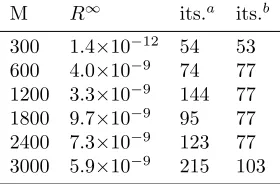
As it turns out, this parabolic game also converges from the ‘zero guess’ (V10 =V20 = 0). On Table 1, the convergence ofR∞over a wide range of finite difference grids (with 301,601, . . . ,3001 nodes) is compiled. In all cases, both initial guesses lead to convergence (to within ε) of Algorithm 2. Nonetheless, the algorithm takes in general fewer iterations when starting from the values of the unilateral parabolic games. (We stress that those on Table 1 are the outer iterations of Algorithm 2. Within each one there is an inner loop of Howard’s iterations. Thus the computational cost scales linearly with the number of outer iterations.)

M R∞ its.a _its.b

300 1.4×10−12 54 53

600 4.0×10−9 74 77

1200 3.3×10−9 144 77 1800 9.7×10−9 _{95 77} 2400 7.3×10−9 _{123 77} 3000 5.9×10−9 _{215 103}

Table 1. Parabolic game: largest residual to QVIs at convergence (R∞) vs. grid points (M+ 1). Iterations to convergence withinε= 10−8_{starting from: zero guess (its.}a_{) and value} functions for one-player games (its.b_{). (Same parameters as in Figure 1.)}

to within ε 1 by a pair of numerical functions which—also approximately—comply with the regularity assumptions of Theorem 1.2.1. As such, they are the (approximate) value functions of the parabolic game.

We conclude this example by illustrating the interplay between the value functions which numerically solve the system of QVIs, the Nash equilibrium derived from them, and the evolution of the optimally controlled underlying. Once the optimal strategies (ϕ∗₁, ϕ∗₂) are available, they can be executed on specific realizations of the game. Sticking to the parameters and numerical solution in Figure 1, Figure 2 depicts one exemplary trajectory of the underlying in the time interval 0≤t≤1000, starting fromx= 0 and subjected to the pair of optimal strategies. For numerical purposes, let us define

ˆ

J_Ti(x;ϕ1, ϕ2) :=_Ex 

 Z T

0

e−ρis_f

i(Xs)ds+ X

k:τi k≤T

e−ρiτki_{φi X}

(τi k)−, δ

i k

+ X

k:τ_kj≤T

e−ρiτkjψ_i X

(τ_kj)−, δ

j k



. (12)

Figure 2. Exemplary trajectory from x= 0 (parameters and solution from Figure 1). The blue and red dashed lines are the intervention thresholds for players 1 and 2, respectively.

Intuitively, ˆJi

T(x;ϕ1, ϕ2) → Ji(x;ϕ1, ϕ2) (defined in (2)) as T → ∞. In fact, after T & 300, the inte-grals in (12) for the parabolic game have essentially attained their asymptotic value. Thus, we simply take Ji(x;ϕ1, ϕ2)≈Jˆ_Ti₌₁₀₀₀(x;ϕ1, ϕ2). With this clarification, Figure 3 shows in particularV1(0) =J1(0;ϕ∗1, ϕ∗2), V2(0) =J2(0;ϕ∗1, ϕ∗2), V1(−1) = J1(−1;ϕ∗1, ϕ∗2), and V2(−1) = J2(−1;ϕ∗1, ϕ∗2), obtained by Monte Carlo sim-ulation.9 _{They compare fairly well with the values of V}

1(0), V2(0), V1(−1) and V2(−1) in Figure 1 obtained by our algorithm. (Even better agreement could be obtained by increasing M in that figure and reducing the discretisation bias and statistical error of the Monte Carlo simulation, but this is good enough to make our point.)

Figure 4. Empty blue [red] circles mean that the player 1 [2] has departed from her optimal strategy while her opponent has not. By virtue of Nash equilibrium, she cannot be (within numerical errors) better off than V1(x) [V2(x)]. Full circles: objective function of the player who does not drop her optimal strategy. Parameters and optimal strategies from Figure 1. (Note that results are subjected to numerical error.)

The Nash equilibrium itself can be visually explored in the following way. For a given starting point x, we keep the optimal strategy for one of the two players, and slightly alter the strategy of the other one. For concreteness, let us assume that player 1 ”moves” (i.e. ϕ1= (1±0.25U)ϕ∗1) while player 2 does not (ϕ2=ϕ∗2). (U is the uniform distribution, and ”±” means with equal chance.) Then, we proceed to calculateJ1_(x;ϕ

1, ϕ∗2) by Monte Carlo simulation as before. By definition of the Nash equilibrium, J1_(x;ϕ

1, ϕ∗2) can not be larger than V1(x). Within numerical tolerance, this is indeed observed in Figure 4, where the blue empty circles (representing J1_{(x;ϕ1, ϕ}∗

2)) do not lie over the blue solid curve (which represents V1(x)). Full blue circles representJ2_{(x;ϕ1, ϕ}∗

2): note that the player who sticks to her optimal strategy may indeed improve overV2(x),

9_{The expected values in (12) are approximated by the mean overN = 200 realizations integrated with the Euler-Maruyama}

should her opponent depart from a Nash equilibrium. (When player 2 is the one who changes, the red circles and red curve in Figure 4 apply instead.)

We stress, however, that Monte Carlo simulations such as those cannotprovethat a pair of strategies form a Nash equilibrium. (At most, they could disprove it.) The only way—in the current state of the theory—of fully characterizing a Nash equilibrium calls for solving the system of QVIs—which Algorithm 2 has now made possible.

4.2.

Capped benchmark game

In this game, we replace the running payoffs of the benchmark by a version capped atK >0:

¯

fi(x) := min{(−1)i−1(x−si), K} (13)

We shall always takeK= 5. Once again, the corresponding unilateral games are well-posed and their solutions can be used as initial guess for the capped benchmark game. As in the previous example, the capped game also seems to converge from the zero guess. Some convergence results are compiled in Table 2. Note that convergence falters with M = 600 andM = 3300 (independently of kmax); we will come back to this later.

M R∞ its.

600 — ∞

900 6.5×10−10 100 1200 8.8×10−9 124 1500 7.4×10−9 78 2700 4.1×10−9 ₉₆ 3000 6.7×10−9 ₁₂₅

3300 — ∞

Table 2. Convergence ofR∞in the capped benchmark game using the zero guess. The hyphen stands for lack of convergence withinε. Same parameters as in Figure 5.

The value functions of the capped benchmark game are a good approximation to those of the benchmark game itself (see Figure 5). This seems to make sense: due to the action of the opponent and forσ K, the discarded portion of the payoff is not very relevant in practice.

4.3.

Benchmark game with educated initial guess

Finally, we tackle the benchmark game, for which an exact solution is available (see Section 1.3). Contrary to the previous examples, Algorithm 2 does not seem to enjoy unconditional convergence here. In fact, when the zero guess was used, it failed to converge more often than not (not reported). In order to construct an adequate initial guess, we first solve for the value functions of the capped benchmark game. Using them as the initial guess, convergence was achieved in every experiment.

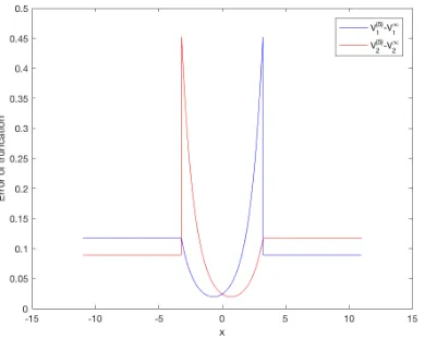
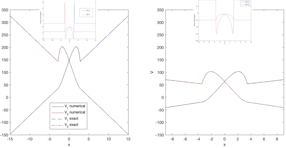
Figure 6. Value functions and Nash equilibrium of two instances of benchmark game. Initial guess: solutions of capped benchmark games (K = 5). Overlaid, error of the initial guess. Parameters: ρ= 0.02,σ= 0.15,s1=−3,s2= 3, c= 100, ˜c= 0, λ= ˜λ= 15,M = 1000 (left); ρ= 0.03,σ= 0.25,s1=−2,s2= 2,c= 100, ˜c= 30,λ= 4, ˜λ= 3,M = 1000 (right).

The result of two experiments are plotted on Figure 6. The numerical approximations can hardly be dis-tinguished from the exact solutions with the naked eye. As it was done with the parabolic game, once again we can retrieve an approximate Nash equilibrium from the numerical solution. For the left figure, this is ϕ∗₁= (−2.82,+∞),1.53−xandϕ∗₂= (−∞,2.82),−1.53−x. When compared with the exact equilibrium, the errors on the corresponding abscissae are smaller than 0.15, i.e., smaller than half the grid step.

difference derivatives grow unbounded as the distance between nodes goes to zero. Figure 7 illustrates this situation. It can be seen that errors continue to be acceptable (far less than 1% relative error in the worst case). We also highlight the fact that the kinks do not seem to bring about oscillations of the numerical solutions around them—the notorious Gibbs’ phenomenon.

M R∞ |error| its.

500 3.8×10−10 _{0.687 126} 1000 1.2×10−9 _{0.805 154} 1500 7.2×10−9 _{0.512 157} 2000 3.5×10−9 _{0.365 172}

2500 — — ∞

Table 3. Convergence of Algorithm 2 for benchmark game. Same parameters as in Figure 6 (left).

M R∞ |error| its.

600 — — ∞

800 9.5×10−10 _{0.023 183} 1000 3.7×10−9 _{0.330 177} 1400 8.7×10−9 _{0.196 159} 1800 6.8×10−9 _{0.121 226} 2200 5.6×10−9 _{0.073 224}

2600 — — ∞

Table 4. Convergence of Algorithm 2 for benchmark game (same parameters as in Figure 6 (right).

5.

Conclusions

We have designed and tested a novel policy iteration algorithm—the first one as far as we know—to numer-ically solve nonzero-sum stochastic impulse games (NZSSIGs). The approach consists in solving a system of quasi-variational inequalities which characterizes the value functions and Nash equilibrium, exploiting a recent theoretical breakthrough in [1].

Our algorithm computes iteratively the approximate solution by partitioning, for each of the players, the discretised spatial domain into an approximate continuation region and an approximate intervention region. They are defined through a relaxation parameter that evolves along the iterations. In the continuation region, we solve one quasi-variational inequality by means of (a generalization of) Howard’s algorithm, whereas in the complement, a gain is computed. A strategy for producing an educated initial guess to start the iterations— which relies on solving two associated, standard impulse control problems—has been presented along with the new Algorithm as well.

We have not carried out a convergence analysis. Instead, we have gathered plenty of numerical evidence showing that the Algorithm can be applied confidently. In particular, we have performed convergence tests on the only available—at the time of writing—example of an analytically solvable NZSSIG. In other test NZSSIGs for which we do not have an analytic solution, we have explored consistency and numerical results on the value functions and Nash equilibrium, also with satisfactory results.

Figure 7. Stagnation of accuracy: the pair withM = 1983 is fully converged (within numerical tolerance); the pair with M = 1984 (overlaid) is not. The insets zoom in on both pairs of functions. Parameters: ρ= 0.02,σ= 0.15,s1=−1,s2= 1,c= 100, ˜c= 30,λ= 4, ˜λ= 3.

to the accuracy attained by our algorithm. On the other hand, its stability is not affected by them. Moreover, in every case the largest pointwise error was perfectly acceptable for the purposes of most applications.

In sum, the new Algorithm offers a means of gaining quantitative insight into applications modelled by NZSSIGs. Natural continuations of the present work include the convergence analysis of the Algorithm, and enriching the discretisation method so as to better capture singularities in the solutions.

Acknowledgments

JPZ was supported by CNPq, FAPERJ, and the Brazilian-French network in Mathematics. FB gratefully acknowledges support from the Finance for Energy Market Research Centre (FiME).

References

[1] R. A¨ıd, M. Basei, G. Callegaro, L. Campi, T. Vargiolu,Nonzero-sum stochastic differential games with impulse controls: a verification theorem with applications, arxiv.org/abs/1605.00039 (2017).

[2] M. Basei,Topics in stochastic control and differential game theory, with application to mathematical finance. Ph.D. Thesis in Mathematics, University of Padova (2016).

[3] R. Bellman,Functional equations in the theory of dynamic programming-XVI: An equation involving iterates. Journal of Mathematical Analysis and Applications30(3), 592-595 (1970).

[4] R. Bellman, Dynamic Programming. With a new introduction by Stuart Dreyfus. Reprint of the 1957 edition. Princeton Landmarks in Mathematics, Princeton University Press, Princeton (2010).

[5] O. Bokanowski, S. Maroso and H. Zidani,Some convergence results for Howard’s algorithm, SIAM J. Numer. Anal., 47(4), 3001-3026 (2009).

[7] J.P. Chancelier, M. Messaoud, A. Sulem,A policy iteration algorithm for fixed point problems with nonexpansive operators. Mathematical Methods of Operations Research65(2), 239-259 (2007).

[8] J.P. Chancelier, B. Oksendal, A. Sulem, Combined stochastic control and optimal stopping, and application to numerical approximation of combined stochastic and impulse control. Tr. Mat. Inst. Steklova237, 149-172 (2002).