Numerical modeling of seismic waves by discontinuous spectral element methods★

P. Lafitte and K. Ramdani, Editors

NUMERICAL MODELING OF SEISMIC WAVES BY

DISCONTINUOUS SPECTRAL ELEMENT METHODS

Paola F. Antonietti

, Alberto Ferroni

, Ilario Mazzieri

, Roberto Paolucci

,

Alfio Quarteroni

, Chiara Smerzini

and Marco Stupazzini

Abstract. We present a comprehensive review of Discontinuous Galerkin Spectral Element (DGSE) methods on hybrid hexahedral/tetrahedral grids for the numerical modeling of the ground motion induced by large earthquakes. DGSE methods combine the flexibility of discontinuous Galerkin meth-ods to patch together, through a domain decomposition paradigm, Spectral Element blocks where high-order polynomials are used for the space discretization. This approach allows local adaptivity on discretization parameters, thus improving the quality of the solution without affecting the compu-tational costs. The theoretical properties of the semidiscrete formulation are also revised, including well-posedness, stability and error estimates. A discussion on the dissipation, dispersion and stability properties of the fully-discrete (in space and time) formulation is also presented. Here space dis-cretization is obtained based on employing the leap-frog time marching scheme. The capabilities of the present approach are demonstrated through a set of computations of realistic earthquake scenar-ios obtained using the code SPEED (http://speed.mox.polimi.it), an open-source code specifically designed for the numerical modeling of large-scale seismic events jointly developed at Politecnico di Milano by The Laboratory for Modeling and Scientific Computing MOX and by the Department of Civil and Environmental Engineering.

∗_{Paola F. Antonietti and Ilario Mazzieri acknowledge the financial support given by SIR Research Grant no. RBSI14VTOS} funded by MIUR - Italian Ministry of Education, Universities and Research. This work has been partially funded by MunichRe and Swissnuclear.

1 _{MOX, Dipartimento di Matematica, Politecnico di Milano,}

Piazza Leonardo da Vinci 32, I-20133 Milano, Italy, e-mail:[email protected]

2 _{MOX, Dipartimento di Matematica, Politecnico di Milano,}

Piazza Leonardo da Vinci 32, I-20133 Milano, Italy, e-mail:[email protected]

3 _{MOX, Dipartimento di Matematica, Politecnico di Milano,}

Piazza Leonardo da Vinci 32, I-20133 Milano, Italy, e-mail:[email protected]

4 _{Dipartimento di Ingegneria Civile ad Ambientale, Politecnico di Milano,}

Piazza Leonardo da Vinci 32, I-20133 Milano, Italy, e-mail:[email protected]

5 _{CMCS, Ecole Polytechnique Federale de Lausanne (EPFL),}

Station 8, 1015 Lausanne, Switzerlande-mail:[email protected]

6 _{Dipartimento di Ingegneria Civile ad Ambientale, Politecnico di Milano,}

Piazza Leonardo da Vinci 32, I-20133 Milano, Italy, e-mail:[email protected]

7 _{Munich Re, Munich, K¨oniginstr. 107, 80802, Germany, e-mail:[email protected]}

c

EDP Sciences, SMAI 2018

Introduction

In the last decades, the scientific research on elastic waves propagation problems modeled through the (visco)elastodynamics equation has experienced a constantly increasing interest in the mathematical, geophysi-cal and engineering communities. In particular, the use of numerigeophysi-cal simulations is a powerful tool to study the ground motion induced by earthquakes in regions threatened by seismic hazards. The distinguishing features of a numerical method designed for seismic wave simulations are: accuracy,geometric flexibility andscalability. To beaccurate, numerical methods must keep dissipative and dispersive errors low. Geometric flexibilityis required since the computational domain usually features complicated geometrical shapes as well as sharp discontinu-ities of mechanical properties.. Additionally, highly realistic earthquake models are typically characterized by domains whose dimension, ranging from hundreds to thousands square kilometers, is very large compared with the wavelengths of interest. This typically leads to a discrete problem featuring several millions of unknowns. As a consequence, parallel algorithms must bescalablein order to efficiently exploit high performance computers.

Historically, one of the first numerical methods employed for the solution of the elastodynamics equation was the finite difference (FD) discretization, see e.g. [8] and [53, 84] for its application to real test cases. Dispersion errors of low order FDs can be mitigated by introducing a staggered grid approach for the velocity-stress formulation of the wave equation as in [77, 111], or by using fourth-order FD schemes as in [22, 35, 75]. An overview of the stability and dispersion properties of three dimensional fourth-order FD scheme can be found in [83] for example. A major challenge for FD methods is related to the treatment of complicated domains and of free-surface or absorbing boundary conditions. Suitable techniques were developed in order to account for surface topography in [99]. We refer the reader to [82] for a comprehensive review of FD schemes applied to seismic waves propagation.

softwares are available for the automatic generation of 3D unstructured tetrahedral grids, able to deal with very complex domains. To exploit this flexibility in the meshing process, high-order or spectral element methods have been extended to tetrahedral elements based on either nodal or modal approximations. Examples of nodal (or Lagrangian) basis functions can be found in [60,110,112], while a modal basis approximation has been originally proposed in [46]. The latter exploits a warped tensor product structure and has the very interesting property of being orthogonal with respect to the L2 _{scalar product, but unfortunately it is not suitable for a global} continuous approximations. This basis has been modified in [105] by introducing the so calledboundary adapted basis in order to enforce the continuity between the elements. Differently from their hexahedral counterpart, both the nodal and the modal approach lead to mass matrices that are no longer diagonal. Therefore, when used with explicit time integrators, the inversion of a global mass matrix at each time-step has an impact on the computational efficiency. For this reason SE on tetrahedral grids encountered up to now a limited interest in the seismology community. An example of a triangular spectral element approximation based on nodal basis functions can be found in [80].

accuracy [39]. The dispersion properties of high-order methods for the scalar wave equations have been analysed in [3] and in [4], where different kinds of DG approximations were considered. In the elastic case, the dispersive behaviour of spectral element methods has been analysed in [101] using a Rayleigh quotient approximation of the eigenvalue problem resulting from the dispersion analysis. DGSE approximations on quadrilateral grids have been investigated using a plane wave analysis in [41] and in [17]. A similar approach has been presented for spectral elements and DGSE approximations on triangular grids [76,78], where different sets of interpolating nodes have been compared, and in [15], where the authors have used the modal boundary adapted functions proposed in [106]. All these works deal with two-dimensional model problems and show that triangular spectral elements feature dispersion and dissipation properties similar to those of the standard tensor product spectral elements. The extension to three dimension is presented in [52], and a similar conclusion can be drawn.

The aim of this work is to present a comprehensive review on numerical modeling of seismic waves based on DGSE methods on hybrid hexahedral/tetrahedral grids. These methods combine the flexibility of discon-tinuous Galerkin methods to connect together, through a domain decomposition paradigm, Spectral Element blocks where high-order polynomials are used. DGSE methods are implemented in SPEED(SPectral Elements in Elastodynamics with Discontinuous Galerkin -http://speed.mox.polimi.it), an open-source code aims at simulating large-scale seismic events in three-dimensional complex media: from far-field to near-field including soil-structure interaction effects. SPEED is jointly developed at Politecnico di Milano by The Laboratory for Modeling and Scientific Computing (MOX) of the Department of Mathematics and the Department of Civil and Environmental Engineering. More precisely, we will review the main advantages of this approach in terms of stability, accuracy, dispersion and dissipation properties, as well as computational costs.

The rest of this paper is organized as follows. In Section 1 we introduce the physical problem and governing equations. A particular emphasis is given to the review of the key ingredients needed to set up a highly realistic model for the numerical simulation of the ground motion induced by large earthquakes, namely, the modeling of the seismic source, absorbing boundaries and suitable damping terms. In Section 2 we present the Discontinuous Spectral Element method for the space discretization coupled with a leap-frog time marching scheme. In Section 3 we revise the theoretical results for the semi-discrete formulation and include the stability and the corresponding error estimates for the semi-discrete problem, whereas Section 4 is concerned with the dissipation, dispersion and stability analysis for the fully discrete scheme. In Section 5 we report some numerical computations of realistic earthquake scenarios in order to fully exploit the capabilities of the present approach. These results have been obtained using the open source code SPEED. Finally, some technical results needed for the theoretical analysis are contained in Appendix A.

1.

Physical problem and governing equations

larger amplitude with respect to body waves.

In the following we introduce the mathematical model that describes the propagation of seismic wdmagniaves within the Earth’s media. We consider a bounded domain Ω⊂_R3_{(representing the portion of the ground where} we study wave propagation), and assume that its boundary is decomposed into three disjoint portions ΓD,ΓN and ΓN R, where we impose the values of displacement, of tractions, and of the fictitious tractions introduced to avoid unphysical reflections, respectively.

Considering a temporal interval (0, T], with T > 0, the dynamic equilibrium equation for a viscoelastic medium subject to an external force leads to the following formulation

         

        

ρu¨+ 2ρζu˙ − ∇ ·σ(u) +ρζ2_{u=f in Ω×(0, T],} u=0 on ΓD×(0, T],

σ(u)n=t on ΓN×(0, T],

σ(u)n=t∗ on ΓN R×(0, T],

u=u0 in Ω× {0},

˙

u=v0 on Ω× {0},

(1)

where ρis the medium density, u=u(x, t) is the displacement field,σ(u) is the stress tensor and f =f(x, t) is a given external load (representing e.g. a seismic source). On the boundary we impose a rigidity condition on ΓD, a traction t =t(x, t) on ΓN and a fictitious traction t∗ = t∗(x, t) on ΓN R. The exact expression of the term t∗ will be discussed later on. Finally, u0 andv0 are smooth initial values for the displacement and the velocity field, respectively. We assume thatρis a uniformly bounded, strictly positive function. In (1) the parameterζ≥0 (usually referred to as damping factor) is a decay factor with the dimension of the inverse of time and it is supposed to be piecewise constant in order to model media with sharp elastic impedance and damping behaviors. The term 2ρζu˙ +ρζ2_{u can also be seen as an alternative or a complement to absorbing} boundary conditions [72]. Usually, in engineering applications, ifζ >0, the viscoelastic behavior of a material is expressed through the adimensional quality factorQ, defined asQ=Q0f /f0, wheref0is a reference frequency andQ0=πf0/ζ.

For the stress tensorσwe use the following constitutive equation (Hooke’s law):

σ(u) =λtr((u))I+ 2µ(u), (2)

where (u) = (∇u+∇T_{u)/2 is the strain tensor,I is the identity tensor,λ=λ(x)∈L}∞_{(Ω) andµ=µ(x)∈}

L∞(Ω) are the first and second Lam´e elastic coefficients, respectively, and tr(·) is the trace operator. By introducing the fourth order Hooke’s tensorD, relation (2) can also be written as

σ(u) =D ε(u), (3)

withD a uniformly bounded and symmetric and positive definite tensor. We recall that the Lam´e coefficients and the mass density are related to the compressional and shear wave velocities through the following relations

cP = s

λ+ 2µ

ρ , cS =

r_µ

ρ, (4)

1.1.

Modelling the seismic source

In this section we discuss the nature of the source termfin (1). In practical applicationsf can be a point-wise force acting on a pointx0 in theithdirection, i.e.

f(x, t) =f(t)eiδ(x−x0), (5)

whereei is the unit vector of theithCartesian axis,δ(·) is the delta distribution, andf(·) is a function of time. The expression off(·) can be selected among different waveforms. A relevant example is the Ricker wavelet [94], defined as

f(t) =f0(1−2π2fp2(t−t0)2)e−π 2_f2

p(t−t0)2_{, (6)}

wheref0is the wave amplitude,fp is the peak frequency of the signal andt0 is a fixed reference time.

Another possible choice of the seismic input is a vertically incident plane wave. In particular, a uniform distribution of body forces along the planez=z0 of the formf(x, t) =f(t)eiδ(z−z0) generates a displacement in theith _{direction of the form}

¯

ui(x, t) = 1 2ρcH(t−

|z−z0|

c )

Z t−|z−_cz0|

0

f(τ)dτ, (7)

where H(·) is the Heaviside function and c (= cP or cS) is the wave velocity, see [57]. Taking the derivative with respect to time of (7) and evaluating the result atz=z0 we can expressf(t) as

f(t) = 2ρc∂u¯i

∂t . (8)

Finally, one of the most important seismic input in earthquake simulation is the double-couple source force. Its mathematical representation is based on the seismic moment tensorm(x, t), defined in [5] as

mij(x, t) =

M0(x, t)

V (sF,inF,j+sF,jnF,i) i, j= 1, ..,3, (9)

wherenF andsF denote the fault normal and the rake vector along the fault, respectively. M0(x, t) describes the time history of the moment release at the point x and V is the elementary volume of the force. The equivalent body force distribution is finally obtained through the relation f(x, t) = ∇ ·m(x, t), see [50]. We recall that the seismic momentM0, measured inN m, can be used to obtain the value of the moment magnitude

Mwof the earthquake as

Mw=

2

3log10M0−6. (10) The moment magnitude scale, expressed through the adimensional valueMw, is used by seismologists to classify the size of earthquakes and it is related to the strain energy released. A variation of one in the moment magnitude scale corresponds to a 2 times increase in terms of the energy released, so that an earthquake of magnitude

Mw≈8 will release 2 times the energy of an earthquake of magnitude Mw≈7.

1.2.

Modelling absorbing boundaries

τ1= [τ1,x, τ1,y, τ1,z]T andτ2= [τ2,x, τ2,y, τ2,z]T be a couple of mutually orthogonal unit vectors that lie on the plane tangent to the boundary, the P3 paraxial absorbing conditions read as

       ∂

∂n(u·n) =− 1 cP

∂

∂t(u·n) + cS−cP

cP

h ∂

∂τ1(u·τ1) + ∂

∂τ2(u·τ2) i

,

∂

∂n(u·τ1) =− 1 cS

∂

∂t(u·τ1) + cS−cP

cP

∂

∂τ1(u·n), ∂

∂n(u·τ2) =− 1 cS

∂

∂t(u·τ2) + cS−cP

cP

∂

∂τ2(u·n).

. (11)

The stress σ∗ = σ∗(u) defined on the absorbing boundary in the local coordinate system (τ1,τ2,n) has the following expression

σ∗_τ1,τ1 = (λ+ 2µ) ∂

∂τ1

(u·τ1) +λ

_∂

∂τ2

(u·τ2) + ∂

∂n(u·n)

, σ∗_τ1,τ2 =µ

_∂

∂τ2

(u·τ1) + ∂

∂τ1 (u·τ2)

,

σ∗_τ2,τ2 = (λ+ 2µ) ∂

∂τ2

(u·τ2) +λ

_∂

∂τ1

(u·τ1) + ∂

∂n(u·n)

, σ∗_τ1,n=µ

_∂

∂n(u·τ1) +

∂ ∂τ1

(u·n)

,

σ∗_n,n= (λ+ 2µ) ∂

∂n(u·n) +λ

∂ ∂τ1

(u·τ1) + ∂

∂τ2 (u·τ2)

. σ∗_τ2,n=µ

∂

∂n(u·τ2) +

∂ ∂τ2

(u·n)

.

By inserting the above espression in (11), the traction termt∗= [t∗_τ

1, t

∗

τ2, t

∗

n]T=σ∗(u)nin the local coordinate system (τ1,τ2,n) reads as





t∗_τ

1

t∗_τ

2

t∗_n

 =    

µ(2cP−cS)

cS

∂

∂τ1(u·n)− µ cS

∂

∂t(u·τ1) µ(2cP−cS)

cS

∂

∂τ2(u·n)− µ cS

∂

∂t(u·τ2) λcS+2µ(cP−cS)

cS

h ∂

∂τ2(u·τ1) + ∂

∂τ1(u·τ2) i

−λ+2µ_c

S

∂ ∂t(u·n)



  

.

Finally, the expression of t∗ in the global coordinate system can be recovered by writing the normal and the tangential derivatives as

∂ ∂n =nx

∂ ∂x+ny

∂ ∂y +nz

∂ ∂z,

∂ ∂τ1

=τ1,x

∂ ∂x+τ1,y

∂ ∂y +τ1,z

∂ ∂z,

∂ ∂τ2

=τ2,x

∂ ∂x+τ2,y

∂ ∂y +τ2,z

∂ ∂z,

and then projecting the resulting vector on the global coordinate system by

t∗(x, t) = 



t∗_x t∗_y t∗z 

= 



τ1,x τ2,x nx

τ1,y τ2,y ny

τ1,z τ2,z nz     t∗ τ1 t∗ τ2

t∗_n



. (12)

Details on the practical choice of the vectors (τ1,τ2) can be found in [28].

2.

Numerical discretization

In this section we describe the numerical approximation of the (weak formulation) of (1) through a Discon-tinuous Spectral Element method coupled with a leap-frog time marching scheme.

For an open, bounded, polygonal domain D⊂R3 and for a non-negative integerswe denote byHs(D) the

L2 _{Sobolev space of ordersand byk · k}

s,D and| · |s,D the corresponding norm and semi-norm. In addition, for

time dependent functions defined on the interval (0, T)

Lq(0, T;Hs(D)) ={v: (0, T)→Hs(D) s.t. Z T

0

kvkq_s,Ddt <+∞}, 1≤q <∞.

cf. [1]. For vector- and tensor-valued functions the above space is defined analogosuly. The spaceC0_{(0, T;H}s_(D)) andC1_{(0, T;H}s_{(D)) are defined analogously.}

LetV ={v∈H1_{(Ω), v=0on ΓD}; the weak formulation of problem (1) read as: ∀t∈(0, T] findu(t)∈V} such that

(ρu¨(t),v)Ω+ (2ρζu˙(t),v)Ω+ (ρζ2u,v)Ω+A(u(t),v) =F(v) ∀v∈V, (13) supplemented with the initial conditionsu(0) =u0 and ˙u(0) =v0, where

A(u,v) = (σ(u), ε(v))Ω, F(v) = (f,v)Ω+ht,viΓN +ht ∗_,vi

ΓN R.

If ΓN R=∅andζ= 0, the above problem is well-posed and its unique solutionu∈C0_{(0, T;V)∩C}1_{(0, T;L}2_(Ω)), provided that ρ ∈ L∞(Ω), u0 ∈ V, v0 ∈ L2(Ω), f ∈ L2(Ω;L2(0, T)) and t ∈ L2(ΓN;L2(0, T)), see for instance [93, Theorem 8.3-1].

2.1.

Partitions and trace operators

We consider a (not necessarily conforming) decomposition TΩ of Ω into L nonoverlapping polyhedral sub-domains Ω`, i.e., Ω = ∪`Ω`, Ω`∩Ω`0 = ∅ for ` 6= `0. On each Ω`, we built a conforming, quasi-uniform

computational mesh Th` of granularity h` > 0 made by open disjoint elements K

j

`, and suppose that each

Kj<sub>`</sub>∈Ω` is the affine image through the mapF_`j:K −→ Kb j

` of either the unit reference hexahedron or the unit reference tetrahedronKb. Given two adjacent regions Ω`±, we define an interior faceF as the non-empty interior

of ∂K+_∩∂K−_{, for some K}± _{∈ T}

h_`±,K

± _⊂Ω

`±, and collect all the interior faces in the setF_hI. Moreover, we

define FD h ,F

N h and F

N R

h as the sets of all boundary faces where displacement, traction or fictitious tractions are imposed, respectively. Implicit in this definition is the assumption that each boundary face can belong to exactly one of the sets FD

h ,F N h , F

N R

h . Finally, we collect all the boundary faces in the set F b

h. To carry out the analysis, we suppose that the following mesh assumption holds, see [55, 88], (see also [44, 45] for the case of highly discontinuous coefficients).

Assumption 2.1. Mesh assumption. For any elementK∈ Th and for any faceF ⊂∂K, it holdshK.hF. We refer to [25], for example, for the weakening of the above assumption and to [11, 24] for for the use of polyhedral-shaped elements.

Let K± _{∈ T}

h_`±,K

± _⊂Ω

`± be two elements sharing a face F ∈ F_hI, and letn± be the unit normal vectors to F pointing outward toK±_{, respectively. For (regular enough) vector and tensor-valued functions v andτ, we}

denote byv± andτ± the traces ofv andτ onF, taken within the interior ofK±_{, respectively, and set}

[[v]] =v+n++v−n−, [[τ]] =τ+n++τ−n−, {v}= v +_+v−

2 , {τ}=

τ+_+τ−

2 , (14)

wherevn= (vT_n+nT_{v)/2. OnF ∈ F}b

h, we set {v}=v, {τ}=τ, [[v]] =vn, [[τ]] =τn.

2.2.

Discontinuous Galerkin Spectral Element approximation

To each subdomain Ω`we assign a nonnegative integerN`, and introduce the finite dimensional space

VN`

h`(Ω`) ={v ∈C

0_{(Ω`) : v K}j

`

◦F<sub>`</sub>j∈[MN`(Kb)]3 ∀ K j

where_MNk₍K_{b) is either the space}

PNk₍K_{b) of polynomials of total degree at mostN}

k onKb, ifKb is the reference tetrahedron, or the space _QNk₍

b

K) of polynomials of degree Nk in each coordinate direction onKb, ifKb is the unit reference hexahedron in _R3_{. We then define the space V}

DG as VDG = Q`V N`

h`(Ω`). The semi-discrete

SIPG approximation of problem (13) reads: ∀t∈(0, T], finduh=uh(t)∈VDG such that

X

Ω`

(ρu¨h(t),v)Ω`+

X

Ω`

(2ρζu˙h(t),v)Ω`+Ah(uh(t),v) +

X

Ω`

(ρζ2uh,v)Ω` =Fh(v) (16)

for anyv∈VDG, subjected to the initial conditionsuh(0) =u0,hand ˙uh(0) =v0,h. The right-hand sideFh(·) is defined as

Fh(v) =X Ω`

(f,v)Ω_`+ht,vi_FN h +ht

∗_,vi

FN R

h v∈VDG, (17)

where we have used the short-hand notation hw,vi_FN

h =

P F∈FN

h hw,viF and hw,viF N R

h =

P F∈FN R

h hw,viF.

The bilinear formAh(·,·) in (16) is defined as

Ah(u,v) =X Ω`

(σ(u), ε(v))Ω_`− h{σ(u)},[[v]]i_FI

h− h[[u]],{σ(v)}iFhI+hη[[u]],[[v]]iFhI, (18)

where, as before,hw,vi_FI

h =

P F∈FI

hh

w,viF.

Remark 2.2. If L = 1, i.e., if there is only one subdomain, FI

h =∅ and the formulation (16)correspond to the classical Spectral Element method. In this case, we will denote the corresponding discrete space as VCG, to highlight that the corresponding semi-discrete solution is globally continuous. On the other hand if L > 1 the discrete solution is piecewise discontinuous across macroelements and (weak) continuity is enforced based on employing, at a subdomain level, the symmetric interior penalty DG (SIPG) method [17]. Notice that here the essential boundary conditions are enforced strongly. In the context of a “fully” DG approach, i.e., the DG paradigm is employed elementwise, relevant applications of the SIPG method to elastic wave propagation problems can be found in [41,97], while in [98] the same problem is solved based on employing the non-symmetric version of the interior penalty method (NIPG) [113]. Other DG methods based on the flux approximation at element interfaces have been considered for the elastodynamics problem in [42, 47, 81] for the stress-velocity formulation and in [10] for both the displacement and the stress-displacement formulation. We refer to [10] for a unified analysis of the h-version of the method and to [13, 15] for the hp-version of the method and its analysis.

2.3.

Fully discrete formulation

In this section we address the issue of integrating in time the semi-discrete formulation (16). By fixing a basis for the discrete spaceVDG, the semi-discrete algebraic formulation of problem (16), reads as

MU¨(t) + (M2+S) ˙U(t) + (A+M3+R)U(t) =F(t), (19)

supplemented with suitable initial conditions U(0) = U0 _{and ˙U(0) = V}0_{. Here, denoting by N}

dof be total number of degrees of freedom, the vector U=U(t)∈_RNdof _{contains, for any timet, the expansion coefficients} of the semi-discrete solution uh(t) ∈VDG in the chosen set of basis functions. Analogously, M,M2,A,M3 are the matrices representations of the bilinear forms

X

Ω`

(ρu¨h(t),v)Ω`,

X

Ω`

(2ρζu˙(t),v)Ω`, Ah(uh(t),v),

X

Ω`

(ρζ2u,v)Ω`,

respectively, cf. (16). When absorbing boundary conditions are included in the model, the matrices S andR

take into account the boundary term ht∗(u),vi_FN R

Finally,Fis the vector representation of the linear functionalFh(·) cf. (16).

For the time integration of the system of second order ordinary differential equations (19), we employ the leap-frog method [91], that it widely employed time integration scheme for the numerical simulation of elastic waves propagation, see for example [21, 31, 67, 81]. Other time integration techniques based on high-order time marching scheme can be employ to discretize in time the (visco)elasdodynamics equation, such as Runge-Kutta methods [64], the ADER-DG method [65] or the space-time DG discretization [12]. With this aim, we subdivide the time interval (0, T] intoNT subintervals of amplitude ∆t=T /NT and we denote by Ui≈U(ti) the approximation of U at time ti =i∆t, i = 1,2, . . . , NT. Whenever ζ = 0, i.e. no dumping is present and ΓN R=∅, thenM2,M3 andRare null and the leap-frog method reads as

MU1= (M−∆t

2

2 A)U

0_{+ ∆tMV}0₊∆t 2

2 F 0_,

MUn+1= (2M−∆t2A)Un−MUn−1+ ∆t2Fn, n= 1, ..., NT −1.

(20)

We notice that (20) involves a linear system with the matrixMto be solved at each time step. The choice the basis functions spanning the space VDG strongly influences the structure of the mass matrixMand, therefore, the computational costs related to the solution of the linear system. Furthermore, the leap-frog method being an explicit second order accurate scheme, to ensure its numerical stability a Courant - Friedrich - Levy (CFL) condition has to be satisfied (see [91]). In this general case, i.e. ζ 6= 0 or ΓN R 6=∅, we set K= M2+S and

Q=A+M3+R. Then, the leap-frog method consists in computing

MU1= (M−∆t

2

2 Q)U

0_{+ (∆tM−}∆t2 2 K)V

0₊∆t2 2 F

0_,

(M+∆t 2 K)U

n+1_{= (2M−∆t}2_Q)Un_{+ (M−}∆t 2 K)U

n−1_{+ ∆t}2_Fn_{, n= 1, ..., N} T −1.

(21)

3.

Analysis of the semi-discrete formulation: stability and error estimates

In this section we review the results on stability, convergence, and corresponding error estimates of the semi-discrete problem (16). For the sake of presentation we assume null tractions, i.e.,t=0, and lack of absorbing boundaries, i.e., ΓN R=∅. Moreover, we assume that each macro region Ω`, ` = 1,2, . . ., consists of a single element, either a hexahedron or a tetrahedron, having size h` and characterized by a polynomial of degreeN`. Notice that in this case the subdomain partitionTΩcoincide with the meshTh, and the skeletonFhI includes all the non-empty intersections between neighboring elements Ω`±. In the following, to avoid the proliferation of

constants, we use the notationa_.bto represent the inequalitya≤Cb, whereC is a given positive constant, independent of the discretization parameters, but that can depend on the material propertiesρ, λ, µ.

Before proceeding we properly define facewise the stabilization functionη∈L∞(FI

h) in (18) as

η|F =α{D}_H

max{N2 `+, N

2 `−}

min{h`+, h<sub>`</sub>−}

, F =∂Ω`+∩∂Ω<sub>`</sub>−, (22)

whereαis a positive constant to be properly chosen. For a piecewise constant tensorD,{D}_H is defined as

{D}_H= 2((n +₎T_D+

3.1.

Well-posedness

Denoting byHs_(T

Ω) the spaceQ`H s_(Ω

`) of piecewiseHs vector-valued functions, for any reals≥0, we recall some useful inequalities.

Lemma 3.1. For any polynomial v of degree N`≥1 overΩ` there hold

|v|m,Ω` .

N<sub>`</sub>2 h`

m−s

|v|s,Ω` 0≤s≤m, (23a)

kvk0,F . _N2

`

h` 12

kvk0,Ω` ∀F ∈ F

I

h, F ⊂∂Ω` (23b) (23c)

We refer, for example, to [2, 23, 26, 100, 104] for further details and for the proof.

We next introduce the following (discretization parameters dependent) norms

kvk2 DG=

X

`

kD1/2ε(v)k2 0,Ω`+kη

1/2_[[v]]k2 0,FI

h ∀v ∈H

1_(TΩ),

|||v|||2_DG=kvk2DG+kη− 1/2

{Dε(v)}k2_0,FI

h ∀

v ∈H2(TΩ),

(24)

with the convention that kwk2 0,FI

h

=P F∈FI

hkwk

2

0,F. Using the trace-inverse inequality (23b) of Lemma 3.1, it can be proved that the norms k · kDG and |||·|||DG are equivalent when restricted to the space VDG. The well-posedness of the semi-discrete formulation (16) easily follows from the following result, cf. [95, Chapter 5], provided alocal bounded variationon the mesh-size and the polynomial degree is assumed, i.e. h`+.h<sub>`</sub>−.h<sub>`</sub>+ andN`+ .N_{`</sub>− .N<sub>`}+ for any pair of neighboring elements Ω_`±, cf. [88] for example.

Lemma 3.2. The bilinear form ADG(·,·) :VDG×VDG−→Rdefined as in (18)satisfies

|ADG(w,v)|_.kwkDGkvkDG, ADG(v,v)&kvkDG2 ∀v,w∈VDG,

where the second estimate holds provided that the parameter α appearing in the definition of the stabilization function cf. (22)is chosen sufficiently large. Moreover,

|ADG(w,v)|.|||w|||DGkvkDG ∀w∈H2(TΩ),∀v ∈VDG.

3.2.

Stability

In this section we present a stability analysis of the semi-discrete formulation (16) in the following (mesh dependent) energy norm

kuh(t)k2

E =kρ1/2u˙h(t)k20,Ω+kρ

1/2_ζuh(t)k2

0,Ω+kuh(t)k 2

DG t∈(0, T] (25)

cf. [10, 13] for the caseζ= 0. Fort= 0, the above definition modifies as

kuh(0)k2E =kρ

1/2_v

0,hk20,Ω+kρ 1/2_ζu

0,hk20,Ω+ku0,hk2DG, (26)

Theorem 3.3(Stability). Let, for any timet∈(0, T]and for a sufficiently large penalty parameterαin (22), uh(t)∈VDG be the solution of problem (16). Iff ∈L2(0, T;L2(Ω)), then

kuh(t)kE .kuh(0)kE +

Z t

0

kf(τ)k0,Ωdτ, 0< t≤T. (27)

Proof. Our proof makes use of some technical results that are proved in Appendix A. By takingv= ˙uhin (16), we obtain

X

Ω`

(ρu¨h,u˙h)Ω`+

X

Ω`

(2ρζu˙h,u˙h)Ω`+

X

Ω`

(σ(uh), ε( ˙uh))Ω_`− h{σ(uh)},[[ ˙uh]]i_FI h

− h[[uh]],{σ( ˙uh)}i_FI

h+hη[[uh]],[[ ˙uh]]iFhI+

X

Ω`

(ρζ2uh,u˙h)Ω` =

X

Ω`

(f,u˙h)Ω_`

that is

1 2

d dt(kuhk

2

E −2h{σ(uh)},[[uh]]iFI

h) + 2

X

Ω`

kρ1/2_ζ1/2_u˙

hk20,Ω` =

X

Ω`

(f,u˙h)Ω_`.

where we have used the definition of the energy norm (25). Integrating the above inequality over the time interval (0, t) we have

kuh(t)k2E−2h{σ(uh(t))},[[uh(t)]]iFI

h+ 4

Z t

0

kρ1/2_ζ1/2_u˙

h(τ)k2L2(Th)d τ =kuh(0)k2E

−2h{σ(uh(0))},[[uh(0)]]i_FI

h+ 2

Z t

0

(f(τ),u˙h(τ))Thd τ.

Since 4R₀tkρ1/2_ζ1/2_u˙h(τ)k2

L2_(Th)d τ ≥0, we get

kuh(t)k2

E−2h{σ(uh(t))},[[uh(t)]]iFI

h ≤ kuh(0)k

2

E−2h{σ(uh(0))},[[uh(0)]]iFI

h+ 2

Z t

0

(f(τ),u˙h(τ))Thd τ.

From Lemma A.3 we get

kuhk2E−2h{σ(uh)},[[uh]]iFI

h &kuhk

2

E, (28)

kuh(0)k2

E−2h{σ(uh(0))},[[uh(0)]]iFI

h .kuh(0)k

2

E. (29)

where the first bound holds provided that the stability parameterαappearing in the definition of the penalization function (22) is chosen large enough. Then

kuh(t)k2

E .kuh(0)k2E+ 2

X

Ω`

Z t

0

(f(τ),u˙h(τ))Ω_`d τ. (30)

The Cauchy Schwarz inequality leads to

2X Ω`

Z t

0

(f(τ),u˙h(τ))Ω_`d τ_.X

Ω`

Z t

0

kf(τ)k0,Ω`kρ

1/2_u˙h(τ)k

0,Ω`dτ ≤

Z t

0

kf(τ)k0,ΩkuhkEdτ. (31)

3.3.

Semi-discrete error estimates

In this section we derive a priori error estimates for the semi-discrete problem (16) in the energy norm (25). We start by recalling the following interpolation estimates (see [19])

Lemma 3.4. For any functionv such thatv|Ω` ∈H

s`<sub>(Ω`),s</sub>

`≥0,`= 1, . . . , L, there existsvI ∈VDG such that

X

Ω`

kv−vIk2r,Ω` .

X

Ω`

h2 min(s`,N`+1)−2r

`

N<sub>`</sub>2s`−2r kvk

2

s`,Ω` ∀r, 0≤r≤s`,

X

Ω`

kv−vIk20,∂Ω` .

X

Ω`

h2 min(s`,N`+1)−1

`

N<sub>`</sub>2s`−1 kvk

2 s`,Ω`,

X

Ω`

k∇(v−vI)k20,∂Ω` .

X

Ω`

h2 min(s`,N`+1)−3

`

N<sub>`</sub>2s`−3 kvk

2 s`,Ω`.

(32)

The above result stands at the basis for the following interpolation bounds.

Lemma 3.5. For any functionv such thatv|Ω` ∈H

s`_(Ω

`),s`≥2,`= 1, . . . , L, there existsvI ∈VDG such that

|||v−vI|||2_DG. X

Ω`

h2 min(s`,N`+1)−2

`

N<sub>`</sub>2s`−3 kvk

2

s`,Ω`. (33)

Moreover, if in addition v,v˙ ∈Hs`_(Ω

`),s`≥2,`= 1, . . . , L, then

kv−vIk2E .

X

Ω`

h2 min(s`,N`+1)−2

`

N<sub>`</sub>2s`−3 kv˙k

2

s`,Ω`+kvk

2 s`,Ω`

. (34)

Proof. We first show (33). With this aim, use Lemma 3.4 to bound each contribution appearing in the definition of the DG norm|||·|||_DG

kD1/2ε(v−vI)k20,Ω. X

Ω`

h2 min(s`,N`+1)−2

`

N2s`−2

`

kvk2s`,Ω`,

kη1/2_[[v−v I]]k20,FI

h .

X

Ω`

h2 min(s`,N`+1)−2

`

N2s`−3

`

kvk2 s`,Ω`,

kη−1/2_{Dε(v−v

I)}k2_0,FI

h .

X

Ω`

h2 min(s`,N`+1)−2

`

N2s`−1

`

kvk2 s`,Ω`.

This yields

|||v−vI||| 2 DG.

X

Ω`

h2 min(s`,N`+1)−2

`

N<sub>`</sub>2s`−3

₁

N`

+ 1 + 1

N2 `

kvk2 s`,Ω` .

X

Ω`

h2 min(s`,N`+1)−2

`

N2s`−3

`

To show (34), we recall the definition (25) of energy normk · kE and employ again the interpolation estimates

of Lemma 3.4 to get

kρ1/2_{( ˙v−v˙}

I)k20,Ω. X

Ω`

h2 min(s`,N`+1)

`

N2s`

`

kv˙k2 s`,Ω`,

kρ1/2_ζ(v−v

I)k20,Ω. X

Ω`

h2 min(s`,N`+1)

`

N2s`

`

kvk2 s`,Ω`,

kv−vIk2DG. X

Ω`

h2 min(s`,N`+1)−2

`

N2s`−3

`

kvk2 s`,Ω`.

Summing up the above contributions we obtain

kv−vIk2E .

X

Ω`

h2 min(s`,N`+1)

`

N2s`

`

kv˙k2 s`,Ω`+

h2 min(s`,N`+1)

`

N2s`

`

kvk2 s`,Ω` +

h2 min(s`,N`+1)−2

`

N2s`−3

`

kvk2 s`,Ω`

!

.X

Ω`

h2 min(s`,N`+1)−2

`

N<sub>`</sub>2s`−3

_h2 `

N3 `

kv˙k2 s`,Ω`+

h2 `

N3 `

kvk2

s`,Ω`+kvk

2 s`,Ω`

.X

Ω`

h2 min(s`,N`+1)−2

`

N<sub>`</sub>2s`−3 kv˙k

2

s`,Ω`+kvk

2 s`,Ω`

,

and the proof is complete.

Theorem 3.6. (A-priori error estimate in the energy norm.) Assume that, for any time t∈[0, T], the exact solution u(t) of problem (1) together with its two first temporal derivatives satisfy u(t)|Ω`,u˙(t)|Ω`,u¨(t)|Ω` ∈

Hs`_(Ω

`),`= 1, . . . , L,s` ≥2. Letuh be the corresponding solution of the semidiscrete DG formulation given in (16), with a sufficiently large penalty parameter αin the definition of the stabilization function (22). Then,

sup t∈[0,t]

kehk2E . sup

t∈[0,T] (

X

Ω`

h2 min(s`,N`+1)−2

`

N2s`−3

`

ku˙k2

s`,Ω` +kuk

2 s`,Ω`

) + Z T 0 X Ω`

h2 min(s`,N`+1)−2

`

N<sub>`</sub>2s`−3 ku¨k

2

s`,Ω`+ku˙k

2 s`,Ω`

dτ. (35)

Remark 3.7. If h= maxΩ<sub>`</sub>h` ≈h`, N` =N for any `= 1, . . . , L, and the exact solution belong to Hs(Ω), with s≥N+ 1, the error estimate above becomes

sup t∈[0,T]

keh(t)k2

E .

h2 min(s,N+1)−2

N2s−3 sup

t∈[0,T]

ku˙k2

s,Ω+kuk2s,Ω + Z T

0

ku¨k2

s,Ω+ku˙k2s,Ω

dτ.

!

(36)

Proof. (Proof of Theorem 3.6.) The discrete formulation (16) isstrongly consistent, that is the exact solution uof (1) satisfies equation (16) for any timet∈(0, T]

X

Ω`

(ρu¨,v)Ω<sub>`</sub>+X Ω`

(2ρζu˙,v)Ω<sub>`</sub> +Ah(u,v) +X Ω`

(ρζ2u,v)Ω_` =Fh(v) ∀v∈VDG. ₍₃₇₎

Subtracting (16) from the above identity and settinge=u−uh, we obtain the error equation

X

Ω`

(ρe¨,v)Ω<sub>`</sub> +X Ω`

(2ρζe˙,v)Ω<sub>`</sub>+Ah(e,v) +X Ω`

(ρζ2e,v)Ω_` = 0 ∀v∈VDG. ₍₃₈₎

We next decompose the error as e = eI −eh, with eI = u−uI and eh = uh−uI, uI ∈ VDG being the interpolant defined as in Lemma 3.5, and rewrite the above identity as

X

Ω`

(ρe¨h,v)Ω`+

X

Ω`

(2ρζe˙h,v)Ω` +Ah(eh,v) +

X

Ω`

(ρζ2eh,v)Ω`

=X Ω`

(ρe¨I,v)Ω`+

X

Ω`

(2ρζe˙I,v)Ω`+Ah(eI,v) +

X

Ω`

(ρζ2eI,v)Ω`. (39)

By taking as test functionv= ˙eh, we get

X

Ω`

(ρe¨h,e˙h)Ω`+

X

Ω`

(2ρζe˙h,e˙h)Ω`+Ah(eh,e˙h) +

X

Ω`

(ρζ2eh,e˙h)Ω`

=X Ω`

(ρe¨I,e˙h)Ω`+

X

Ω`

(2ρζe˙I,e˙h)Ω`+Ah(eI,e˙h) +

X

Ω`

(ρζ2eI,e˙h)Ω`, (40)

that is 1 2 d dt

kρ1/2_e˙

hk20,Ω+kρ 1/2_ζe

hk20,Ω+kehk2DG−2h{σ(eh)},[[eh]]iFI h

+ 2kρ1/2_ζ1/2_e˙ hk20,Ω=

X

Ω`

(ρe¨I,e˙h)Ω`+

X

Ω`

(2ρζe˙I,e˙h)Ω`

+Ah(eI,e˙h) + X

Ω`

(ρζ2eI,e˙h)Ω`. (41)

Using the definition of the energy norm (25) and the Cauchy-Schwarz inequality to bound the terms on the right hand side we obtain

1 2

d dt

kehk2E −2h{σ(eh)},[[eh]]iFI h

+ 2kρ1/2ζ1/2e˙hk20,Ω

≤ ke˙IkEkehkE+ 2kρ1/2ζ1/2e˙Ik0,Ωkρ1/2ζ1/2e˙hk0,Ω+Ah(eI,e˙h) + X

Ω`

(ρζ2eI,e˙h)Ω`. (42)

Thanks to the Young’s inequality we have that 2kρ1/2_ζ1/2_e˙

Ik0,Ωkρ1/2ζ1/2e˙hk0,Ω≤ kρ1/2ζ1/2e˙Ik20,Ω+kρ

1/2_ζ1/2_e˙ hk20,Ω, and therefore the above bound can be rewritten as

1 2

d dt

kehk2E −2h{σ(eh)},[[eh]]iFI h

+kρ1/2ζ1/2e˙hk20,Ω

≤ ke˙IkEkehkE+kρ1/2ζ1/2e˙Ik20,Ω+Ah(eI,e˙h) + X

Ω`

Observing thatkρ1/2_ζ1/2_e˙

hk0,Ω≥0, integrating in time between 0 andt, and using thateh(0) =uh(0)−uI(0) = 0

1 2

kehk2E−2h{σ(eh)},[[eh]]iFI h

≤

Z t

0

ke˙IkEkehkEdτ+

Z t

0

kρ1/2ζ1/2e˙Ik20,Ωdτ

+ Z t

0

Ah(eI,e˙h)dτ+ Z t

0 X

Ω`

(ρζ2eI,e˙h)Ω`. (44)

Employing Lemma A.3 we obtain

1 2kehk

2

E .

Z t

0

ke˙IkEkehkEdτ +

Z t

0

kρ1/2ζ1/2e˙Ik20,Ωdτ + Z t

0

Ah(eI,e˙h)dτ + Z t

0 X

Ω`

(ρζ2eI,e˙h)Ω`dτ. (45)

We next estimate the last two terms on the right hand side. For the first one, the integration by parts formula (78) together with the observation thateh(0) =uh(0)−uI(0) =0, and Lemma 3.2 lead to

Z t

0

Ah(eI,e˙h)dτ =Ah(eI(t),eh(t))− Ah(eI(0),eh(0))− Z t

0

Ah( ˙eI,eh)dτ (46)

.|||eI|||DGkehkDG+

Z t

0

|||e˙I|||DGkehkDGdτ (47)

.|||eI|||DGkehkE+

Z t

0

|||e˙I|||DGkehkEdτ, (48)

where in the last step we have used the definition of the energy norm (25). Analogously, for the second term

Z t

0 X

Ω`

(ρζ2eI,e˙h)Ω`dτ =

X

Ω`

(ρζ2eI(t),eh(t))Ω`−

X

Ω`

(ρζ2eI(0),eh(0))Ω`−

Z t

0 X

Ω`

(ρζ2e˙I,eh)Ω`dτ (49)

.keIkEkehkE +

Z t

0

ke˙IkEkehkEdτ. (50)

By substituting the above two bounds in (45) we get

1 2kehk

2

E .(keIkE+|||eI|||DG)kehkE+

Z t

0

kρ1/2_ζ1/2_e˙

Ik20,Ωdτ+ Z t

0

(ke˙IkE +|||e˙I|||DG)kehkEdτ. (51)

From the Young’s inequality, it follows

(keIkE +|||eI|||DG)kehkE ≤(keIkE +|||eI|||DG) 2₊1

kehk

2

E ≤2(keIk2E +|||eI||| 2 DG) +

1

kehk

2

E, (52)

and therefore, we can therefore chose= 4C beingC the hidden constant in (51) and obtain from (51)

1 4kehk

2

E .keIk2E +|||eI||| 2 DG+

Z t

0

kρ1/2ζ1/2e˙Ik20,Ωdτ+ Z t

0

(ke˙IkE+|||e˙I|||DG)kehkEdτ. (53)

By applying the Gronwall’s lemma A.1 with a constantGdefined as

G= sup t∈[0,T]

keIk2E+|||eI|||2_DG+ Z t

0

kρ1/2_ζ1/2_e˙ Ik20,Ωdτ

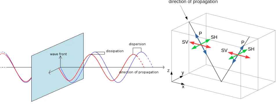
Figure 1. Left: Example of a traveling wave (blue line) and its numerical approximation (red

line). Right: Decomposition of a seismic wave into SH, SV and P components.

we obtain

kehk2E . G+

Z t

0

(ke˙Ik2E+|||e˙I||| 2

DG)dτ. (55)

The interpolation estimates of Lemma 3.4 and Lemma 3.5 lead to

G_. sup

t∈[0,T] (

X

Ω`

h2 min(s`,N`+1)−2

`

N<sub>`</sub>2s`−3

ku˙k2

s`,Ω` +kuk

2 s`,Ω`+

Z t

0

ku˙k2 s`,Ω`dτ

)

, (56)

ke˙Ik2E +|||e˙I|||2_DG. X

Ω`

h2 min(s`,N`+1)−2

`

N<sub>`</sub>2s`−3 ku¨k

2

s`,Ω`+ku˙k

2 s`,Ω`

, (57)

Therefore we obtain

sup t∈[0,T]

kehk2E . sup

t∈[0,T] (

X

Ω`

h2 min(s`,N`+1)−2

`

N2s`−3

`

ku˙k2

s`,Ω`+kuk

2 s`,Ω`+

Z t

0

ku˙k2 s`,Ω`dτ

)

+ Z T

0 X

Ω`

h2 min(s`,N`+1)−2

`

N<sub>`</sub>2s`−3 ku¨k

2

s`,Ω`+ku˙k

2 s`,Ω`

dτ, (58)

and the proof is complete.

4.

Dispersion, dissipation and numerical stability analysis

The aim of this section is to present an analysis of the dispersion, dissipation and stability properties for the fully discrete numerical scheme.

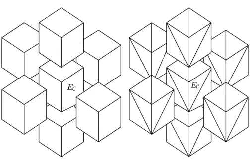
Figure 2. Periodic reference element EC and periodic reference patterns: hexahedral grid (left) and tetrahedral grid (right).

in a three dimensional elastic medium can be decomposed into: i) a pressure wave (P-wave) with velocitycP inducing a displacement in the same direction of the propagating wave;ii)a shear wave (S-wave) with velocity

cS inducing a displacement in a direction transversal to the propagating wave. Additionaly, S-waves can be further decomposed into a vertical component (SV-wave), inducing a motion on a plane perpendicular to the wave direction, and a horizontal component (SH-wave), inducing a transversal motion on a horizontal plane containing the wave direction, see [5, 103] and Figure 1 (right). The Von Neumann analysis [33, 63] investigates the properties of numerical solutions approximating plane waves of the form

u(x, t) =aei(k·x−ωt), (59)

propagating in an unbounded domain and looks for quantitative estimates of the dispersion and the dissipa-tion errors. Here, a = [a1, a2, a3]T ∈R3 represents the amplitude of the wave, ω the angular frequency, and

k= 2π/L(cosθcosφ,sinθcosφ,sinφ) the wave vector, beingLthe wavelength, andθandφthe angles between the propagating direction and the coordinate axes. The physical wave can be recovered by taking the real part of (59).

To comply with unboundedness, we consider problem (1) posed over a reference domain EC and impose

periodic boundary conditions on its boundary, see Figure 2. In the case of a hexahedral tessellation, the smallest periodic grid is made by a single cube, i.e. EC = (−1,1)3 whereas for tetrahedral grids it is composed

by six tetrahedra, Figure 2. Given that we are considering a DG spectral element method, the interelement jump and average contributions are assembled at the interfaces betweenEC and its neighbors (periodic reference

pattern), see Figure 2. Assuming, without loss of generality, no seismic source (i.e. f ≡0), no dumping factor (i.e. ζ= 0) and no reflecting boundaries (i.e. ΓN R=∅), the semi-discrete problem (19) becomes

   

  

M1U¨(t) +AU(t) =0,

U(0) =U0,

˙

U(0) =V0,

(60)

where U0 _{= ae}i(k·x) _{and V}0 _=−iωaei(k·x)_{. Follow the approach of [15, 17, 41, 52, 76, 78] we impose periodic} boundary conditions by introducing a suitable projection matrixΠand we obtain from (60)

e

where Me =ΠTM1Πand eA=ΠTAΠ. We next consider the fully discrete formulation based on employing the leap-frog time integration scheme (20) to (61); the analogous results for the semidiscrete case can be found in [52]. Following [6], we substitute (59) into (61) and we obtain

e

M(e−iωtj+1_−2e−iωtj _+e−iωtj−1₎U 0

∆t2 +Aee

−iωtj_U0_{=0, j = 1, ..., N}

T−1. (62)

The above system can be rewritten as

e

M(2−e−iω∆t−eiω∆t) 4 ∆t2U

0₌ e

AU0. (63)

Now, using the following relation

2−e−iω∆t−eiω∆t= 2(cos(ω∆t)−1) = 4 sin2

ω∆t

2

,

we obtain a generalized eigenvalue problem of the form

e

AU0= ΛMUe 0, (64)

where the eigenvalues Λ are related to the angular frequencyω at which the wave travels in the grid through the relation

Λ = 4 ∆t2sin

2_(ω∆t

2 ). (65)

We will use this after solving the eigenvalue problem in order to derive the grid-dispersion relations as it will be shown later on. We remark that for three dimensional seismic modeling only three eigenvalues in (64) have a physical meaning as they are related to shear and pressure waves, cf. [39, 41] for the bidimensional case. All the other eigenvalues correspond to nonphysical modes, see e.g. [33] for the one dimensional case.

4.1.

Dispersion errors

The relative dispersion errors are given by

eP =

cP,h

cP

−1, eS =

cS,h

cS

−1, (66)

wherecP andcSare the P- and S-wave velocities (see (4)) whereascP,handcS,hare the corresponding numerical wave velocities whose expression is given by

cP,h=

h ωP,h

2πδ , cS,h= h ωS,h

2πδ , (67)

2 4 6 8 10−16

10−13

10−10

10−7

10−4

10−1

∆t= 0.001

∆t= 0.0001

N |eP

|

2 4 6 8

10−16

10−13

10−10

10−7

10−4

10−1

∆t= 0.001

∆t= 0.0001

N

|

eS

|

(a) Hexahedral grid

2 4 6 8

10−16

10−13

10−10

10−7

10−4

10−1

∆t= 0.001

∆t= 0.0001

N |eP

|

2 4 6 8

10−16

10−13

10−10

10−7

10−4

10−1

∆t= 0.001

∆t= 0.0001

N

|

eS

|

(b) Tethrahedral grid

Figure 3. Computed dispersion errorseP (left) andeS(right) versusN for ∆t= 0.001,0.0001. The continuous lines refers to the semi-discrete approximation.

10−2 ₁₀−1

10−12

10−10

10−8

10−6

10−4

10−2

∆t= 0.001

∆t= 0.0001

δ |eP

|

10−2 ₁₀−1

10−12

10−10

10−8

10−6

10−4

10−2

∆t= 0.001 ∆t= 0.0001

δ |eS

|

(a) Hexahedral grid

10−2 ₁₀−1

10−12

10−10

10−8

10−6

10−4

10−2

∆t= 0.001

∆t= 0.0001

δ |eP

|

10−2 ₁₀−1

10−12

10−10

10−8

10−6

10−4

10−2

∆t= 0.001

∆t= 0.0001

δ |eS

|

(b) Tethrahedral grid

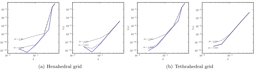
Figure 4. Computed dispersion errorseP (left) and eS (right) versus the sampling ratioδfor ∆t= 0.001,0.0001. The continuous lines refers to the semi-discrete approximation.

eigenvalues approximatingωSV andωSHare not exactly the same but their difference is negligible, cf. [101,115]. In the following we will select ΛS as that eigenvalue, between the two physically relevant ones, that leads to the worst approximation ofcS.

4.2.

Dissipation errors

We next move to the dissipation analysis that is carried out by studying the amplitude of the numerical displacement. By considering as the exact solution of (60) the unitary amplitude plane wave, we can express its amplitude as |ei(k·x−ωt)_|=etIm(ω)_{. Since the physical wave satisfies Im(ω) = 0, its amplitude is equal to 1} for all times t. On the contrary, the numerical wave will have in general Im(ωh)6= 0. Then, we say that the scheme is non dissipative if Im(ωh) = 0, whereas it is dissipative if Im(ωh)<0. In the generalized eigenvalues problems (64) the mass and the stiffness matrices are symmetric and positive definite. Therefore, the computed eigenvalue are all real, leading to a scheme that does not suffer from dissipation errors.

4.3.

Numerical stability

In this section we briefly analyze the stability properties of the fully discrete scheme (21), focusing as before on the case where no dumping is present, i.e. ζ= 0, and no reflecting boundaries are considered, i.e. ΓN R=∅. According to the Courant, Friedrichs and Lewy (CFL) condition, the leap-frog scheme is stable provided that the time step ∆tsatisfies

∆t≤CCF L

h cP

, (68)

wherehis the granularity of the computational grid andcP is the velocity of pressure waves. The constantCCF L depends both on the material properties ρ, λ, µ and on the polynomial degree N. We consider a generalized eigenvalue problem of the form (64) but rescaled on the reference elementKb

b

AU0= Λ0MUb 0, (69)

where Λ0 = (h/∆t)2_sin2_{(ωh∆t/2) and introduce the stabilization parameter q = c}

P∆t/h. The following in-equality holds

q2Λ0=c2_P

sin

_ω h∆t

2 2

≤c2_P, (70)

or, equivalently,

q≤ √cP

Λ0 =CCF L(Λ). (71)

As shown in [40], Λ0 depends on the wave vector kand therefore on the values of the incident anglesφandθ. Thus, (71) can be formulated as

q≤c∗(λ, µ)_p 1 Λ0

max

, (72)

where Λ0_max is the maximum eigenvalue of (69), taken with respect the values of φ and θ. The constant c∗

depends on the Lam´e parameters λand µas well as on the penalty paramenter αappearing in the definition of the stabilization function (22), more precisely it is proportional toα−1/2_{, see [14].}

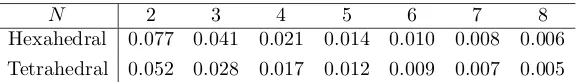
We next present some numerical experiments to give a quantitative estimate of the CFL bound expressed in term of the stability parameter q. The material properties considered are the same as in the previous section and the stability parameterα= 10. In Table 1 we report the computed value of qas a function onN

N 2 3 4 5 6 7 8 Hexahedral 0.077 0.041 0.021 0.014 0.010 0.008 0.006 Tetrahedral 0.052 0.028 0.017 0.012 0.009 0.007 0.005

Table 1. Computed stability parameterqas a function ofN= 2, ..,8 on both the hexahedral

and tetrahedral reference elements.

5.

Numerical experiments

5.1.

Layer over half space benchmark

In this example we apply our method to a more challenging test case, known in the literature as the LOH (Layer Over a Half-space) test. This problem has been proposed in [38] and it has been used as reference benchmark for different numerical codes for the elastodynamics [37, 47]. The domain Ω consists of a rectangle of dimension (−15,15)×(−15,15)×(0,17)km, with a 1km layer (L) on the top surface (see Figure 5). The material properties of the layer and of the halfspace (HS) are summarized in Table 2.

30km

30km

17km

1km x

y

z

Figure 5. LOH test case. Computational domain. The red dot denotes the position of the

seismic source.

Layer ρ[kg/m3] cP [m/s] cS [m/s] L 2600 4000 2000 HS 2700 6000 3464

Table 2. LOH test case. Material properties.

The seismic source is modelled as a point double-couple,f =∇δ(x−xs)M(t), located at the pointxs= (0,0,2)

km, where the moment rate M(t) = M0

t t2 0

e−tt_{0, being M}

0 = 1018 N m the scalar seismic moment and

t0 = 0.1 s a relaxation time controlling the frequency and the amplitude of the seismic source. Finally, we impose a free surface condition on the top surface and absorbing conditions on the remaining ones, while for the time integration we fix ∆t= 0.0002s.

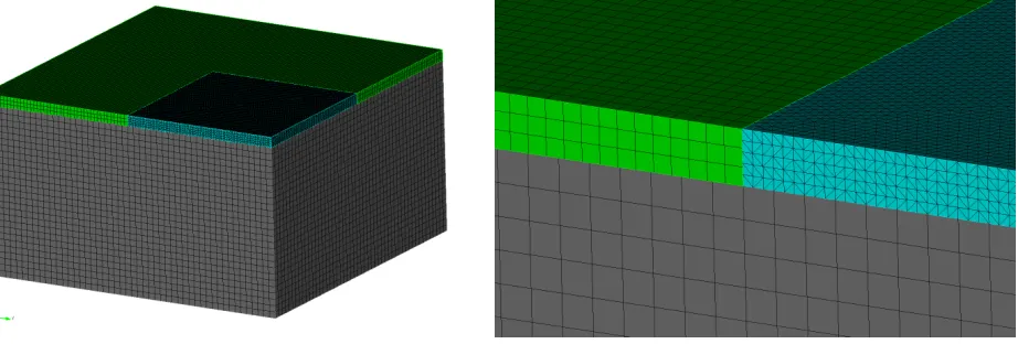
Figure 6. Left: computational grids for the LOH test case B). Right: detail of the grid at the

interface between the layer and the half space. We can observe the non-conforming interface between the tetrahedral and the hexahedral grid.

84141 hexahedral elements. We employN = 5 for the elements in the half-space andN = 4 for the elements in the layer. The resulting number of degrees of freedom Ndof inside the hexahedral region is approximately 10 million. Regarding the region meshed with tetrahedral elements, we consider the three following configurations:

A) h≈150 m,N = 3,Ndof = 6.0×105, B) h≈200 m,N = 3,Ndof = 9.8×105, C) h≈200 m,N = 4,Ndof = 2.3×106.

We also remark that the grid of each portion of the domain has been built independently from the others, leading to a grid characterized by non conforming interfaces on the skeleton.

To compare the results obtained with the reference solution we report the time histories of the velocity field measured at a receiver located at the point (6,8,0) km. For each component of the velocity we also compute the relative seismogram misfitE through the formula

E=

Pns i=1( ˙u

h_{(ti)−u˙(ti))}2 Pns

i=1u˙(ti)2

, (73)

wherens is the number of time samples in the seismogram, ˙uh_{(ti) is the numerical velocity at the timet} i and ˙

u(ti) is the value of a quasi-analytical solution, which can be found in [18, 38].

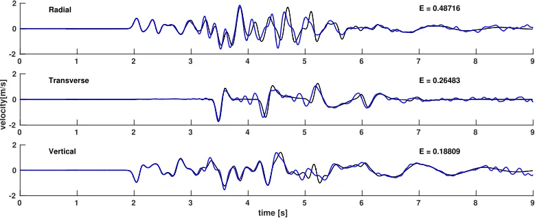
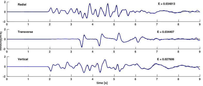
In Figures 7, 8 and 9 we report the radial, transversal and vertical components of the velocity field recorded at the point (6,8,0)km. From the velocity histories we observe that the setting for the case A provides the worst approximation. The numerical solution, indeed, presents spurious oscillations, in particular in the transversal component. This oscillatory effect is probably due to dispersion effects caused by the low order approximation. In both the cases B and C the oscillations are mitigated and the value of the seismic misfit is below the 10% and 4%, respectively. The small oscillations that can be appreciated after 6.5sare probably due to reflecting waves generated by the artificial boundaries. From the numerical results, we can conclude that our approach seems to have at least the same accuracy of other finite difference and finite element numerical approaches [37, 48, 79].

Finally, in Table 3 we report the number of elements and of degrees of freedom used in the tetrahedral portion of the layer, together with the computational times needed for the set-up, the assembly of the mass matrix and to compute the solution at each time step. The results show that the setting used for test case B (h≈200 m,

0 1 2 3 4 5 6 7 8 9 -2

0 2

Radial E = 0.48716

0 1 2 3 4 5 6 7 8 9

-2 0 2

velocity[m/s]

Transverse E = 0.26483

0 1 2 3 4 5 6 7 8 9

time [s]

-2 0 2

Vertical E = 0.18809

Figure 7. LOH test case. Grid configuration A. Velocity field recorded at (6,8,0) km. The

blue line represents the numerical solution, the black line represents the quasi-analytical solu-tion.

0 1 2 3 4 5 6 7 8 9

-2 0 2

Radial E = 0.093605

0 1 2 3 4 5 6 7 8 9

-2 0 2

velocity[m/s]

Transverse E = 0.081861

0 1 2 3 4 5 6 7 8 9

time [s]

-2 0 2

Vertical E = 0.059989

Figure 8. LOH test case. Grid configuration B. Velocity field recorded at (6,8,0) km. The

blue line represents the numerical solution, the black line represents the quasi-analytical solu-tion.

Case Nb. elem. Polynomial degree Ndof Set up [s] Mass ass. [s] Time/step [s] E [%] A 4.2e+4 2 6.0e+5 11.7e+3 0.7 4.3 31 B 2.0e+3 3 9.8e+5 7.1e+3 300 3.2 7.88 C 2.0e+3 4 2.3e+6 7.7e+3 6.2e+3 10.8 3.2

Table 3. LOH test case. Numerical settings, computational times and average seismic misfit

0 1 2 3 4 5 6 7 8 9 -2

0 2

Radial E = 0.034813

0 1 2 3 4 5 6 7 8 9

-2 0 2

velocity[m/s]

Transverse E = 0.034407

0 1 2 3 4 5 6 7 8 9

time [s]

-2 0 2

Vertical E = 0.027606

Figure 9. LOH test case. Grid configuration C. Velocity field recorded at (6,8,0) km. The

blue line represents the numerical solution, the black line represents the quasi-analytical solu-tion.

5.2.

Comparison with a Spectral Element discretization

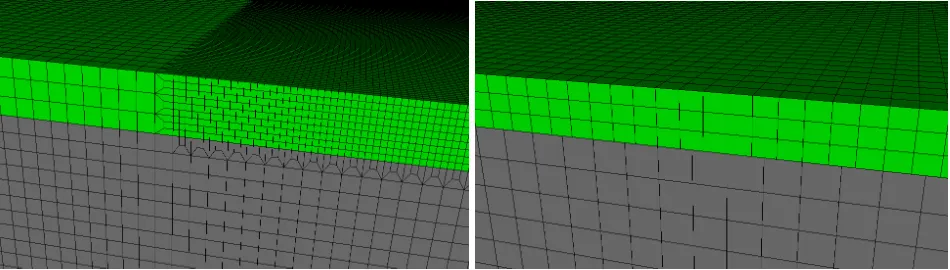
In this section we want compare the overall computation cost of a DGSE discretization with respect to a SE one. In this respect, we consider for the LOH problem described in Section 5.1 two different computational models: the first one consists of a hexahedral conforming mesh, while the second one of a hexahedral non conforming mesh, cf. Figure 10. In Table 4 we report the discretization parameters employed for both com-putational models. For completeness, in Figure 10 a zoom of the computational domains is shown, while in

Case Mesh Elements Mesh Type h(HS) h(L) N Nel Ndof E [%] SE Hex Conforming 300 m 100-300m 4 814833 ≈150·106 ₁ DGSE Hex Non-Conforming 600 m 400 m 5 70228 ≈27·106 _1.3

Table 4. LOH test case: main characteristics of the SE and DGSE numerical models.

Case Cores ∆t Steps Time/step [s] SE 512 5.e-4 18000 0.23 DGSE 512 5.e-4 18000 0.25

Table 5. LOH test case. computational parameters of the analysis performed at Fermi cluster (Cineca).

Figure 11 the radial, transversal and vertical components of the velocity field recorded at the point (6,8,0)km

Figure 10. Detail of the grids at the interface between the layer and the half space. SE (left)

and DGSE (right) computational model.

Figure 11. Velocity field recorded at (6,8,0)km. SE (left) and DGSE (right) solutions.

comparison between the SE and DGSE methods as well as scalability analysis of the DGSE approximation we refer the reader to [36, 79].

5.3.

Earthquake scenarios for the area around Beijing

The accurate evaluation of seismic risk scenario in large urban areas is based on suitable approaches for earthquake ground motion prediction. However, the empirical tools that are most often used for this purpose neglect the specific tectonic and geological conditions in which the urban area lies, thus producing in many cases significant underestimations of the earthquake ground motion intensity. An overview of applications of physics-based numerical modelling approaches to large urban areas was presented in [85]. Specifically, SPEED has been applied so far to several case studies, including Christchurch and Wellington (New Zealand), Santiago (Chile), Istanbul (Turkey), and several urban areas in Italy. In this section, we aim at summarizing results obtained from a large set of earthquake scenario simulations in Beijing (China).

Figure 12. Contour of depth of sedimentary base. Superimposed black line represents the

projection of Shunyi-Qianmen-Liangxiang fault considered in the present work.

Segment Strike Dip Lmax Wmax Fault Origin Top Depth (◦) (◦) [km] [km] (LAT [◦N], LON [◦E]) [m] South 30 80 35.6 30 (39.5586, 116.0657) 31.7 Middle 48 80 29.7 30 (39.8387, 116.2696) 51.9 North 44 80 24.9 30 (40.0211, 116.5248) 38.8

Table 6. Geometric parameters of the Shunyi-Qianmen-Liangxiang fault. Fault Origin is

defined as the point of the fault at zero strike and zero dip.

years, destructive earthquakes have occurred in the area around Beijing, with magnitude varying from Mw 6 toMw 6.5, cf. [58]. For these reasons, the characterization of strong ground motion plays a crucial role for the risk assessment studies in this large urbanized area.

Setup of the 3D computational model

The 3D numerical model for the Beijing area was set up exploiting: i) the topography model; ii) depth of sedimentary base; iii) the kinematic seismic fault model; iv) and the 3D velocity profiles. For the elevation model, a freely-available digital elevation dataset of CGIAR-CSI for the Beijing region has been extracted and downloaded from the website http://www.cgiar-csi.org (with a precision of roughly 90×90m, for east-west and north-south directions around Beijing city), while the depth of sedimentary base model has been derived from the digitalization of the map proposed in [54], as shown in Figure 12.

The seismic fault considered is named Shunyi-Qianmen-Liangxiang fault, lying just through the downtown of Beijing (Figure 12, cf. also Figure 13 left.). This is a quasi-normal segmented fault (with dip angle of about 80◦_{), consisting of three main segments with different strike angles. The total length of the fault is about 90km,}

Figure 13. Left: Vs,30 map adopted in the present work. Right: cs model in the first layer of the domain (depth<2km).

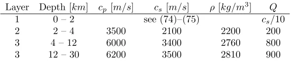
Layer Depth [km] cp [m/s] cs[m/s] ρ[kg/m3] Q 1 0 – 2 see (74)–(75) cs/10 2 2 – 4 3500 2100 2200 200 3 4 – 12 6000 3400 2760 800 3 12 – 30 6200 3500 2810 900

Table 7. Horizontally stratified crustal model, cf. [54].

In order to define the 3D soil model, theVs,30map provided by MunichRe company, cf. [7], and the depth of sediment base obtained previously, see Figure 13, were used. In particular, in the first layer (0 to 2 km depth), we defined different velocity profiles (inm/s) as follows

  

 

cs=Vs,30+ 5 p

|z−ztop|, cp= 1.6cs, forVs,30>= 600m/s

cs=Vs,30+ 10 p

|z−ztop|, cp= 1.6cs, forVs,30<600 m/sandz >=zsed,

cs= 800 + 10 p

|z−ztop|, cp= 2000 + 15 p

|z−ztop|, forVs,30<600 m/sandz < zsed,

(74)

where ztop and zsed represent the projection of a generic point with coordinate z into the surface and the sediment base, respectively. Similarly, for the soil density (kg/m3_{) we consider the following profiles}

  

 

ρ= 1800 + 5p|z−ztop|, forVs,30>= 600m/s

ρ= 1530 + 5p

|z−ztop|, forVs,30<600 m/sandz >=zsed,

ρ= 1800 + 5p|z−ztop|, forVs,30<600 m/sandz < zsed.

(75)

Figure 13 (right) shows the cs model obtained for the first layer. The properties of the underlying bedrock layers (depth>2km) have been selected in agreement with [54]. The quality factor Q is estimated directly by thecsvalues and is assumed to be proportional to frequency, see Section 1, for the target valueQ=cs/10 to be obtained atf = 1 Hz. The 3D velocity model is summarized in Table 7.

Figure 14. Left: Computational domain of Beijing region adopted in the present work.

Shunyi-Qianmen-Liangxiang fault system included in the domain. Right: µ−γandζ−γcurves adopted for the first layer of the model whereVs,30<= 400m/sandztop<=z <=ztop−300m, in a non-linear elastic approach.

Mw Rupture Area (km2) Simulated scenarios 6.5 24×12 15

6.9 36×18 10 7.3 54×24 5

Table 8. Simulated scenarios grouped for magnitude.

wavelength for non-dispersive wave propagation in heterogeneous media by the SE approach (see [79]), and considering a maximum frequencyfmax= 1.5Hz, the model consists of 859,677 hexahedral elements, resulting in approximately 160 million degrees of freedom, using a fourth order polynomial approximation degree. The conforming mesh has a size varying from a minimum of 150m, on the top surface, up to 600mat 4km depth and reaching 1800m in the underlying layers.

Summary of simulated scenarios

A total of 30 scenarios were simulated by varying the magnitude, from 6.5 up to 7.3, the kinematic slip distribution, the hypocenter location and the location of the rupture area. The simulations were performed on the Marconi cluster`ı at CINECA, Italy (http://www.cineca.it/en/content/marconi). Each simulation takes around 12 hours on 512 cores. A summary of the seismic scenarios, grouped according to the magnitude, is given in Table 8.