Mortality Modelling and Forecasting using Cross-Validation Techniques

using Cross-Validation Techniques

Wouter van Wel*

Abstract

This paper investigates how accurately several predictive models perform in the field of mortallity modelling and forecasting, using cross-validation techniques. The main models used in this paper are the well-known Lee-Carter model and the Heligman-Pollard model. Furthermore, some extensions will be investigated: a distinction between the male and female population, extension to a few other countries, the effects of increasing the size of the ”training set” and forecasting without re-estimatingktfor the Lee-Carter model and a weighted estimation for the Heligman-Pollard model.

Keywords: Lee-Carter, Heligman-Pollard, mortality modelling, mortality forecasting, cross-validation

1 Introduction

In the last century, human mortality rates have steadily declined, leading to longer life

expectan-cies. Although, there are differences across gender, age and countries. Mortality trends have been affected by several events, such as the Spanish Flu and World War II, but also by changes

in human behaviour, like smoking and alcohol consumption. Such things present risks for

insurers, who might have not taken this into account. This is what makes mortality modelling, and in particular mortality forecasting, so important these days.

* _{Wouter van Wel received a bachelor degree in Econometrics and Operations Research at Maastricht University}

in 2014. Currently he is taking a master in Econometrics and Operations Research at Maastricht University (specialisation: Econometrics).

Since the publication of the Gompertz law of mortality in 1825, several methods have been

proposed for the modelling of mortality rates. However, this paper will only focus on the

well-known Lee-Carter model and the Heligman-Pollard model. The main objective is to investigate how accurately these two models will perform in practice, using Dutch data1. This will be done

using cross-validation techniques. The first step is to divide the complete data set into two

subsets: the first is used for analysis (modelling and forecasting), the latter for comparison [6]. Additional to the main analysis, a few extensions will be applied: a distinction between the

male and female population, extension to Danish and Norwegian population, the effects of

increasing the size of the ”training set” and forecasting without re-estimatingktfor the Lee-Carter model; and a weighted estimation for the Heligman-Pollard model. All these results will be

compared with the original results for both models with Dutch data.

The paper is structured as follows. Chapter 2 provides an extensive description of the Heligman-Pollard model and the Lee-Carter model. Chapter 3 discusses the main analysis of

these two models and compares their results. Chapter 4 adresses all extensions described before and discusses their results. Finally, Chapter 5 draws conclusions.

2 Methods

Nowadays, many methods have been proposed to model and forecast mortality rates, ranging from an extrapolative approach to GLM methods and the Lee-Carter method; for an extensive

review, see Booth and Tickle [2]. The Lee-Carter is probably the best known method for mortality

forecasting these days. Among the many parameterisation functions which have been proposed, the Heligman-Pollard model is well known.

2.1 Heligman-Pollard Model

The Heligman-Pollard model [3] is an eight-parameter parameterisation function.

Parameterisa-tion funcParameterisa-tions (laws of mortality) are one-factor models which try to depict the age pattern of mortality. However, they are of limited use in mortality forecasting due to unstable parameter

time series and interdependencies [2]. The Heligman-Pollard model is defined as:

qx

px

=A(x+B)C +Dexp[−E(lnx−lnF)2] +GHx (2.1)

whereAtoHare the eight parameters, andpx = 1−qx.

1

The first component, a rapidly declining exponential, reflects the fall in mortality during the

early childhood years. A measures the level of mortality,C measures the rate of decline in

childhood mortality andB is an age displacement. The second component, a function similar to the lognormal, reflects accident mortality for male and accident plus maternal mortality for the

female population. The ”accident hump” can be found in all populations, usually between the

ages of 10 and 40.F indicates location,E spread andDthe severity. The last component, also known as the Gompertz exponential, reflects the rise in mortality at adult ages, or senescent

mortality.Grepresents the base level of senescent mortality andH reflects the rate of increase

of that mortality. Figure 1 provides a nice illustration of all three components.

Figure 1– The mortality curve and its three components. Australian national male mortality, 1970-72 [3].

Mortality forecasting using the Heligman-Pollard model is ideally done by multivariate time

series methods. In this paper however, univariate time series methods are used. The time

function:

110

X

x=0

(qx ˙ qx

−1)2 (2.2)

whereqxis the fitted value at agexandq˙xis the observed mortality rate. The best ARIMA model

is then fit to each parameter by looking at the Akaike Information Criterion (AIC) and the Bayesian Information Criterion (BIC). After forecasting each of the parameters separately, all forecasted

parameters are plugged back into the Heligman-Pollard model to obtain the forecasted mortality

rates.

2.2 Lee-Carter Model

The Lee-Carter model is a two-factor model specified by Lee & Carter [5]. In contrast to parameterisation functions, which try to represent the age pattern of mortality, the Lee-Carter

method is a principal components approach, whereby the age pattern is estimated from the data. The Lee-Carter model is specified as:

lnmx,t=ax+bxkt+εx,t (2.3)

wheremx,t is the central mortality rate at agexin yeart;axis the average log-mortality at age

x;bxmeasures the response at agexto change inkt;ktrepresents the overall level of mortality in yeart; andεx,t is the residual.

Estimation of the parameters is done as follows: ax is estimated by averaging log-mortality rates over time andbxandktvia singular value decomposition (SVD), a method for approximating

a matrix as the product of two vectors. In order to get a unique solution, two constraints are

necessary: thebxshould sum to 1 and thektto 0. Without these constraints, the model in (2.3) is not identifiable. For example, the model with (ax, bx, kt) would be the same as the model

with(ax, bx/c, ckt), for any constantc. Hereafter, the estimatedktis adjusted in such a way that

the observed total deaths equal the total deaths "“predicted” by the model in each year. Doing so compensates the effect of taking log-rates, because ages at which deaths are high receive

greater weights [1]. The adjusted estimatedktis modelled as a simple random walk with drift:

kt=kt−1+d+et (2.4)

where d is the drift parameter and et is an error term. Forecasted mortality rates are then

3 Main Analysis

This chapter will discuss how the mortality rates are modelled and forecasted using the

Heligman-Pollard model and the Lee-Carter model. Furthermore, the results of both methods will be analysed and compared. In the main analysis, only Dutch data (total population) will be

considered. The complete data set (1850-2009) is used, the period 1850-1979 is used as

”training set” and the period 1980-2009 as ”testing set”. Figure 2 gives a graphical overview of the mortality curves for the Dutch population over the entire period from 1850 until 2009.

3.1 Heligman-Pollard Model

The complete estimation of the parameters for the Heligman-Pollard model has been done

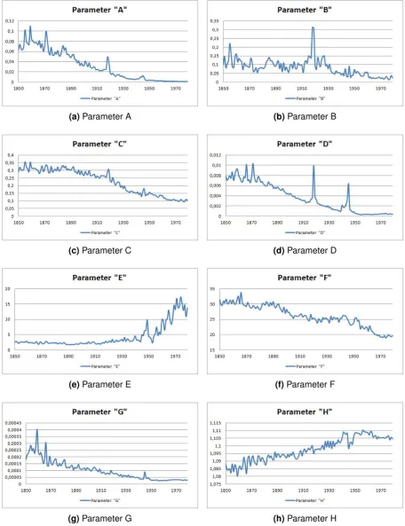
in Microsoft Excel, using its Solver function. Figure 4 shows time series graphs of all eight

parameters. In some of the graphs, one will notice outliers in the years 1918-1919 and 1945. These are due to, respectively, the Spanish Flu and World War II. In order to receive a better

forecast, these outliers have been removed.

Modelling and forecasting of the eight parameters has been done using Eviews. Univariate time series methods have been used to model all parameters according to ARIMA models.

Table 1 provides a small overview of these ARIMA models.

log(A) log(B) C log(D) log(E) F log(G) H

ARIMA (2,1,2) (0,1,1) (3,1,4) (4,1,4) (4,1,4) (2,1,1) (2,1,1) (6,1,0)

AIC -0.9301 0.4326 -5.7585 -0.8471 -0.4825 2.5657 -1.0587 -9.3076

BIC -0.8164 0.4776 -5.5756 -0.6403 -0.2757 2.6567 -0.9677 -9.1445

Table 1– ARIMA models for the parameters of the Heligman-Pollard model.

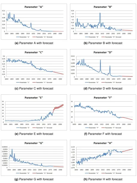
Using these ARIMA models, each parameter is forecasted. The forecasted mortality rates are then obtained by plugging these forecasted parameters back into the model. Time series graphs

of all eight parameters with their forecast are illustrated in figure 3.4.

3.2 Lee-Carter Model

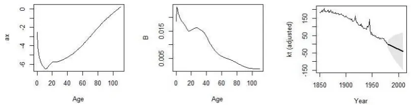
Forecasting mortality rates via the Lee-Carter model has been done using the demography package [4], available for R. Estimates forax andbx and a time series graph for the adjustedkt,

with 95% confidence interval, are shown in Figure 3.

The left graph in Figure 3 shows the average over time log-mortality, whereas the middle graph

shows how a certain age group responds to a change in the adjustedkt, which is illustrated in

the lower-right graph.

The graphs in Figure 6 and 7 give a small illustration of how the actual and forecasted mortality

curve of the Dutch population in the first year (1980) and the last year (2009) of the forecasting

period look like.

3.3 Comparison

The comparison of the Heligman-Pollard and Lee-Carter model for Dutch data will be based on

the mean absolute percentage error (MAPE). Figure 8 and 9 show the MAPE of the log-mortality

for both models. A big disadvantage of the Heligman-Pollard model is that big errors occur at ages 0 and 110+, which obviously can be seen from the graph in Figure 8. The Lee-Carter model

does not have this disadvantage, but seems to have higher errors at adolescent ages. Comparing

their overall fit, the Heligman-Pollard model seems to fit better to the Dutch data, which is a striking result, since the Heligman-Pollard model is supposed to be worse in forecasting than the

(a)Parameter A (b)Parameter B

(c)Parameter C (d)Parameter D

(e)Parameter E (f)Parameter F

(g)Parameter G (h)Parameter H

(a)Parameter A with forecast (b)Parameter B with forecast

(c)Parameter C with forecast (d)Parameter D with forecast

(e)Parameter E with forecast (f)Parameter F with forecast

(g)Parameter G with forecast (h)Parameter H with forecast

Figure 6– Actual and forecasted mortality curve for the Netherlands in 1980 (Lee-Carter).

Figure 8– MAPE Heligman-Pollard for Netherlands, total population (1980-2009).

4 Extensions

This chapter will elaborate on the extensions mentioned before. For the Heligman-Pollard model,

a weighted estimation will be investigated. For the Lee-Carter model, a distinction between male and female population will be made for the Dutch data, Denmark and Norway will be used for

forecasting, the effect of increasing the ”training set” will be considered and forecasts will be

made without re-estimating thektseries.

4.1 Heligman-Pollard Extensions

4.1.1 Weighted Heligman-Pollard Estimation

In Chapter 3, we noticed big errors at ages 0 and 110+ for the Heligman-Pollard model. In order to reduce these errors, a weighted estimation is used. The weights are defined by the number of

deaths in a certain year for a certain age group (dx,t), as proposed by Wilmoth [7]. Since the variance oflnmx,tis roughly1/dx,t, bigger weights should be given to observations with a higher

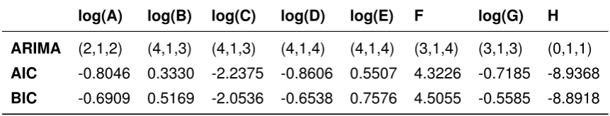
value ofdx,t, since these observations have a lower variance. Table 2 provides an overview of

the ARIMA models selected for each parameter in case of a weighted estimation.

log(A) log(B) log(C) log(D) log(E) F log(G) H

ARIMA (2,1,2) (4,1,3) (4,1,3) (4,1,4) (4,1,4) (3,1,4) (3,1,3) (0,1,1)

AIC -0.8046 0.3330 -2.2375 -0.8606 0.5507 4.3226 -0.7185 -8.9368

BIC -0.6909 0.5169 -2.0536 -0.6538 0.7576 4.5055 -0.5585 -8.8918

Table 2– ARIMA models for the parameters of the weighted Heligman-Pollard model.

The results of using a weighted estimation are illustrated in Figure 10. The purpose of this

adjustment seems not to be fully achieved; the big error at age 0 has been reduced significantly,

but the error at age 110+ has even slightly increased, this being the results of a relatively low weight for age group 110+, as there are few deaths at this age. Furthermore, large errors

at age 14 and 15 arise, almost reaching 50%. Besides these two big errors, this adjustment

seems to reduce the errors at ages 0-20, but performs worse at ages 21-70. Considering ages 71-110+, the weighted estimation seems to slightly reduce the errors, except for ages 89-105

and 110+. The overall fit seems to be slightly worse than before, leading to the conclusion that

Figure 10– Comparison MAPE Heligman-Pollard unweighted/weighted for Netherlands, total popu-lation (1980-2009).

4.2 Lee-Carter Extensions

4.2.1 Distinction between male and female population

The first extension which will be investigated is the distinction between male and female

popula-tion for the Dutch data. The length of the ”training” and ”testing” set will remain the same. The

time-averages ofaxandbx and the time series of the adjustedktfor the Dutch male and female population are reported in respectively Figure 11 and 12.

The comparison for this extension is based on the mean percentage error (MPE). Figure 13 il-lustrates the MPE for the Dutch male and female population. The result is kind of strange. For

the ages 0-20, the MPE for the male population shows high positive errors up to approximately

120%, then slowly fading to 0. For ages 40-110+, the male MPE seems to fluctuate around 10%. However, for the female population, one observes high negative errors at ages 0-60, up

to approximately -60%, then fading to 0 aswell. For the ages 70-110+, the female MPE shows

Figure 11– Estimates forax,bxand the adjustedktfor the Dutch male population.

4.2.2 Extension to Denmark and Norway

The second extensions of the Lee-Carter model includes forecasting using Danish and

Nor-wegian data. These two countries were picked for a certain reason, namely that they cover the same time-horizon as the Dutch data, whereas for all other countries, the data starts after

1850. In this way, and by having the same length of the ”training” and ”testing” set for all three

countries, it makes sense to compare the results. The time-averages ofaxandbx and the time series of the adjustedktfor the Danish and Norwegian population are reported in respectively

Figure 14 and 15.

The comparison for this extension is based on the MAPE. Figure 16 shows the MAPE for the Netherlands, Denmark and Norway (total population). The big error hump at adolescent ages

appears to be smaller for both Norway and Denmark, for the latter it has even decreased untill

approximately 40%. Considering ages 70-90, both Norway and Denmark have bigger errors than the Netherlands. At ages 100-110+, the MAPE’s for Denmark and the Netherlands are

close to eachother, but Norway seems to produce a bit higher errors. We can conclude that the

Norwegian data seems to overall fit slightly better than the Dutch data. Although, the Lee-Carter model seems to fit best to the Danish data, where the MAPE at adolescent ages is considerably

Figure 12– Estimates forax,bxand the adjustedktfor the Dutch female population.

4.2.3 Increasing the ”training set”

This extension of the Lee-Carter looks into the effect of increasing the ”training set”. The Dutch

data will be used again and the ”training set” will be increased twice, once by 10 years and once

by 20 years. One would expect that increasing the ”training set” would reduce the errors, as there is more information available for analysis (i.e. modelling and forecasting). The time-averages of

axandbxand the time series of the adjustedktfor both the 10 and 20 years increased ”training

sets” are reported in respectively Figure 17 and 18.

The comparison for this extension is again based on the MAPE and is illustrated in Figure 19.

The red line shows the MAPE from the main analysis, as in Chapter 3. The black and green

line respresent, respectively, the 10 and 20 years increase of the ”training set”. This means that instead of forecasting over a period of 30 years (1980-2009), now only 20 (1990-2009)

and 10 years (2000-2009) are being forecasted. Looking at the 10 years increase, there is

a slight decrease of errors at ages 0-60 and a somewhat bigger decrease at ages 80-110+. Although, there is a small increase at ages 65-75. Considering the 20 years increase, the errors

at adolescent ages seem to decrease even more and there’s also a slight decrease at ages

Figure 13– Comparison MPE Lee-Carter for Netherlands, male and female population (1980-2009).

better forecasts using the Lee-Carter model, although for ages around 60-80 the MAPE seems

to increase.

4.2.4 Forecasting without adjusting thektseries

Every Lee-Carter forecast in this paper used the adjustment for thektseries, as described in

section 2.2. This section will investigate the effect of not using this adjustment for the Dutch

data. One would expect that errors will rise for age groups with a relative high number of deaths, because their weights will now be lower. Hence, the observed number of deaths will now not be

equal to the number of deaths predicted by the model. Figure 20 shows the time-averages ofax

andbx and the time serieskt, without adjustment.

The comparison for the last extension is again based on the MAPE and is illustrated in

Figure 21. The results show what we expected: a rise in the MAPE for age groups with a relative

high number of deaths. There is a significant larger MAPE for ages 0-10 and also for ages 60-110+ there is an increase. For the adolescent ages, we observe considerably lower errors,

Figure 14– Estimates forax,bxand the adjustedktfor Denmark, total population.

5 Conclusions

In this paper, the Heligman-Pollard model and the Lee-Carter model have been applied to the

field of mortallity modelling and forecasting. Cross-validation techniques were used to measure how accurately these two models performed in practice. The main analysis in Chapter 3 was

based on data from the Netherlands (total population) where the data set was divided into the

”training set” (1850-1979) and the ”testing set” (1980-2009).

The results, based on the MAPE, showed that the Heligman-Pollard model seemed to fit

better to the Dutch data than the Lee-Carter model, although big errors at age 0 and 110+

occured. This is not in line with the general conclusion that parameterisation functions, such as the Heligman-Pollard model, usually do not perform well in forecasting mortality rates.

Chapter 4 focussed on the extensions: a distinction between the male and female population,

extension to Danish and Norwegian population and the effects of increasing the size of the ”training set” for the Lee-Carter model; and a weighted estimation for the Heligman-Pollard model.

All these results were compared with the original results for both models with Dutch data. The goal of the weighted Heligman-Pollard estimation was to reduce the big errors at age 0

and 110+. The results showed that the error at age 0 was indeed significantly reduced, but on

the other hand the error at age 110+ even slightly increased. Furthermore, big errors at age 14 and 15 arised.

The distinction between the Dutch male and female population for the Lee-Carter model led

to remarkable results: high positive errors for the male population ages 0-20 and high negative errors for the female population ages 0-60, completely different from the MAPE for the total

Dutch population.

Extending the Lee-Carter model to Denmark and Norway led to the conclusion that the Lee-Carter model seems to fit best to the Danish data: the big errors at adolescent ages were

reduced significantly, but at ages 70-90 the MAPE increased. The Norwegian data fitted slightly

better than the Dutch data, but large errors remained.

Investigating the effect of an increase in the ”training set” was done by considering three

cases: the original one, a 10-year increase and a 20-year increase, leading to a forecast period

of respectively 30, 20 and 10 years. The results showed that increasing the ”training set” leads to smaller errors at adolescent ages, but there was a significant increase in the MAPE at ages

60-80.

The last extension focussed on the effect of not using the adjustment for thektseries. This meant that the observed number of deaths each year would not be equal to the number of

deaths observed by the model. The results showed that for ages 0-10 and 60-110+ there was

References

[1] H. Booth, R.J. Hyndman, L. Tickle, and P. de Jong. Lee-carter mortality forecasting: a

multi-country comparison of variants and extensions. Demographic Research, 15(9):289–310, 2006.

[2] H. Booth and L. Tickle. Mortality modelling and forecasting: a review of methods. Annals of

Actuarial Science, 3:3–43, 2008.

[3] L. Heligman and J.H. Pollard. The age pattern of mortality. Journal of the Institute of

Actuaries, 107(434):49–80, 1980.

[4] R.J. Hyndman. demography: Forecasting mortality and fertility data, r package. http:

//www.robhyndman.info/Rlibrary/demography, 2006.

[5] R.D. Lee and L.R. Carter. Modelling and forecasting u.s. mortality. Journal of the American Statistical Association, 87(419):659–671, 1992.

[6] P. Refaeilzadeh, L. Tang, and H. Liu. Cross validation. Encyclopedia of Database Systems.,

Springer, 2009.

[7] J.R. Wilmoth. Computational methods for fitting and extrapolating the Lee-Carter model