M. Belhaq, P. Lafitte and T. Leli`evre Editors
SYNCHRONIZATION AND CONTROL OF A NETWORK OF COUPLED
REACTION-DIFFUSION SYSTEMS OF GENERALIZED FITZHUGH-NAGUMO
TYPE
∗Benjamin Ambrosio and M.A. Aziz-Alaoui
1R´esum´e. Nous consid´erons un r´eseau de syst`emes de r´eaction-diffusion de type FitzHugh-Nagumo g´en´eralis´es. Nous nous int´eressons au comportement asymptotique et `a la synchronisation du r´eseau. Ces r´esultats nous permettent d’´etendre d’autres r´esultats obtenus pour un type particulier de syst`emes de FitzHugh-Nagumo.
Abstract. We consider a network of reaction diffusion systems of generalized FitzHugh-Nagumo type, where the cubic function is replaced by a polynomial function with odd degree. We deal with asymptotic behaviour and synchronization of the whole network. These results extend a previous work in which we considered particular systems of FitzHugh Nagumo type.
1.
Introduction
Let us denote bywtthe time derivative of the functionw. The FitzHugh-Nagumo model,
(
xt=c(F(x) +y+z)
yt= 1
c(x−a+by)
whereF is a cubic function with positive leading coefficient,zconstant, anda, b, c >0, is a simplification of the well known Hodgkin-Huxley model describing the propagation of action potential in neurons, see for example, [1–3,5,7]. In [9], we considered a network of coupled reaction-diffusion systems of the following FitzHugh-Nagumo type (FHN),
ǫut = f(u)−v+du∆u
vt = u−δv+dv∆v (1)
where,
f(u) =−u3+ 3u,
∗This work was supported by Region Haute Normandie, France, and FEDER-RISC. 1 LMAH, FR-CNRS-3335,
Universit´e de Le Havre ISCN
PRES Normandie Universit´e, BP 540, 76058, Le Havre Cedex, FRANCE
c
EDP Sciences, SMAI 2013
and where ǫ, δ >0, are small parameters. In this case, the underlying (ODE) part of system (1) induces an asymptotic evolution to a unique limit cycle for the trajectories diferent from (0,0). We showed some results on asymptotic behaviour and synchronization for the network. Here, we will generalize some of these results. Let us consider a network of coupled reaction diffusion systems of the following generalized FHN type,
ǫut = f(u)−v+du∆u+γ
vt = au−bv+dv∆v+µ (2)
where,
f(u) = p
X
k=1
dkuk
is a polynomial function of odd degree with negative leading coefficient, dp <0, p≥ 3. The parameter ǫ > 0 is small. The underlying (ODE) part of system (1) can induce a very more complicated asymptotic behaviour. We assume thata, b, du are positive, anddv is non negative. We look for solutionsu=u(x, t),v=v(x, t) on a smooth bounded domain Ω⊂Rn, with zero-flux Neumann boundary conditions on the boundary of Ω :
∂u
∂ν =
∂v ∂ν = 0,
where ν denotes the exterior normal to the boundary. The coupling is chosen such that, for all i = 2, ..., N, subsystem (ui−1, vi−1) drives subsystem (ui, vi). This means that the whole system reads as,
ǫu1t = f(u1)−v1+du1∆u1+γ1
v1t = a1u1−b1v1+dv1∆v1+µ1
.. .
ǫuit = f(ui)−vi+dui∆ui+αi(ui−1−ui) +γi vit = aiui−bivi+dvi∆vi+βi(vi−1−vi) +µi
.. .
ǫuN t = f(uN)−vN +duN∆uN +αN(uN−1−uN) +γN vN t = aNuN −bNvN+dvN∆vN +βN(vN−1−vN) +µN
(3)
whereαi, βi≥0, fori= 2, ..., N.
2.
Analytical results
2.1.
Space homogeneous asymptotic behaviour
Let (u, v) be the solution of system (2), then we have the following result, Th´eor`eme 2.1. Let,
M = sup x∈R
f′(x),
and λ be the smallest non zero eigenvalue of the Laplacian operator (−∆) with zero flux Neumann boundary conditions. If,
M −λdu<0, (4)
then,
lim
t→+∞ ||(u−u¯||L2(Ω)+||v−v¯||L2(Ω)
where,
¯
u(t) =
R
Ωu(x, t)dx
|Ω| , ¯v(t) =
R
Ωv(x, t)dx
|Ω| . Moreover,u¯,¯v are solutions of the following system,
ǫu¯t = f(¯u)−¯v+γ+g(t) ¯
vt = au¯−b¯v+µ (6)
whereg(t)is a function going to 0 with exponential rate whent goes to+∞ . D´emonstration. Let,
φ(t) = 1 2 aǫ
Z
Ω
|∇u|2+
Z
Ω
|∇v|2 ,
then,
˙
φ =
Z
Ω
(ǫa∇u∇ut+∇v∇vt) =
Z
Ω
(a∇u∇(f(u)−v+du∆u) +∇v∇(au−bv+dv∆v)) =
Z
Ω
(a(f′(u)|∇u|2−du(∆u)2)−b|∇v|2−dv(∆v)2)
Now, we use the following spectral property of laplacian operator with zero-flux Neumann boundary conditions, see for example [10],
Z
Ω
(∆u)2≥λ Z
Ω
∇|u|2.
Then,
˙
φ ≤ a
Z
Ω
M|∇u|2−λdu
Z
Ω
|∇u|2
−b Z
Ω
|∇v|2−λdv
Z
Ω
|∇v|2
≤ a(M−λdu)
Z
Ω
|∇u|2−(λdv+b)
Z
Ω
|∇v|2.
Now, sinceλdu> M we have,
˙
φ≤ −2 min
λdu−M
ǫ , λdv+b
φ,
and thus,
φ(t)≤φ(0)e−c1t
where,
c1= 2 min
λdu−M
ǫ , λdv+b
.
Furthermore,
||u−u¯||2L2(Ω)+||v−¯v||2L2(Ω)≤
1
λ Z
Ω
|∇u|2+
Z
Ω
|∇v|2
≤ 2
λmax
1
aǫ,1
which implies (5). In the remaining of the proof, we show that ¯uet ¯v are solutions of (6). We have,
ǫu¯t = |Ω1|RΩf(u)−¯v+γ ¯
vt = au¯−b¯v+µ thus,
ǫu¯t = |Ω1|
R
Ω(f(u)−f(¯u)) +f(¯u)−¯v+γ
¯
vt = au¯−bv¯+µ. Let us denote,
g(t) = 1 |Ω|
Z
Ω
(f(u)−f(¯u)).
Then, we obtain :
ǫu¯t = g(t) +f(¯u)−¯v+γ ¯
vt = au¯−b¯v+µ. But,
|g(t)| = | 1 |Ω|
Z
Ω
(f(u)−f(¯u))|
≤ L
|Ω|
Z
Ω
|u−u¯|
≤ L
|Ω|12
||u−u¯||L2(Ω),
where,
L= sup t∈R+
|f′(¯u(t))|,
since from a result in [6], we know that (u, v)∈L∞(Ω)×L∞(Ω). It follows that : lim
t→+∞g(t) = 0.
Which completes the proof.
Let (ui, vi), 1≤i≤N be the solution of system (3)
Th´eor`eme 2.2. Let λbe the smallest non-zero eigenvalue of the Laplacian operator, with zero flux Neumann boundary conditions. Assume that,
M−λdu1 <0 andM−λdui−αi<0 ∀i∈2, .., N , (7)
(8) then,
lim t→+∞
N
X
i=1
||ui−u¯i||L2(Ω)+||vi−v¯i||L2(Ω)= 0, (9)
where,
¯
ui(t) =
R
Ωui(x, t)dx
|Ω| , v¯i(t) =
R
Ωvi(x, t)dx
ǫu¯it = f(¯ui)−v¯i+γi+gi(t) +αi(¯ui−1−u¯i) ¯
vit = aiu¯i−biv¯i+µi+βi(¯vi−1−¯vi) (10)
and where, gi(t)→0 whent→+∞with exponential rate decay.
D´emonstration. It comes from an induction argument, by using similar techniques as those given in the proof of Theorem 2.1. More precisely, let,
φi= 1 2
ǫai
Z
Ω
|∇ui|2+
Z
Ω
|∇vi|2
,
we show that for alli∈1, ..., N there exists positive constantsKi, ci such that,
φi(t)≤Kie−cit.
From the proof of Theorem 2.1, we know that this result is true fori= 1, that is,
φ1(t)≤φ1(0)e−c1t.
Let us assume that the result is true untili−1, by algebraic computations we obtain, ˙
φi ≤ ai(M−λdui−αi+ αiκi
2 )
Z
Ω
|∇ui|2−(λdvi+bi+ βi
2)
Z
Ω
|∇vi|2+ai
αi 2κi
Z
Ω
|∇ui−1|2+
βi 2
Z
Ω
|∇vi−1|2
≤ ai(M−λdui−αi+ αiκi
2 )
Z
Ω
|∇ui|2−(λdvi+bi+ βi
2)
Z
Ω
|∇vi|2+s1Ki−1e−ci−1t
≤ −s2φ+Ki−1e−ci−1t
whereκi is a positive constant satisfying
κi<2
λdui+αi−M αi
,
ands1= max(
αi
ǫκi
, βi),s2= 2 min(
λdui+αi(1−
κi
2)−M
ǫ , λdvi+bi+
βi
2),Ki−1,ci−1 are positive constants. By integration, this yields,
φi(t)≤Kie−cit.
The remaining of the proof is similar as this of Theorem 2.1.
2.2.
Synchronization
D´efinition 2.3. LetSi= (ui, vi). We say thatSi andSj synchronize if, lim
t→+∞(||ui−uj||L2(Ω)+||vi−vj||L2(Ω)) = 0.
The quantity,
is called the norm of synchronization error betweenSiandSj. LetS= (S1, S2, ..., SN). We say thatSsynchronize if,
lim t→+∞
N−1
X
i=1
(||ui−ui+1||L2(Ω)+||vi−vi+1||L2(Ω)) = 0
The quantity,
N−1
X
i=1
(||ui−ui+1||2L2(Ω)+||vi−vi+1||2L2(Ω))
12
is called the norm of synchronization error ofS.
Let us consider the system (3) withdui =duj,dvi =dvj andbi =bj =b, ai=aj =a,γi=γj,µi=µj, for
alli, j∈ {1, ..., N}. Let us recall thatf is a polynomial function of odd degree with negative leading coefficient,
f(u) = p
X
k=1
dkuk, dp<0, p≥3.
Let,
M = sup
u∈B,x∈R p
X
k=1
f(k)
k! (u)x k−1,
whereB is a compact interval in which u1 remains strictly.
Th´eor`eme 2.4. If,
αi> M, i= 2, ..., N,
then the network S= ((u1, v1),(u2, v2), ...,(uN, vN))synchronize in the sense of definition (2.3). D´emonstration. Let
ψi(t) = 1 2 aǫ
Z
Ω
(ui−ui−1)2+
Z
Ω
(vi−vi−1)2.
Our proof is based on an induction idea. We show that for alli∈2, ..., N, ψi(t)≤Kie−cit.
We first consider the subsystem (u2, v2). By derivatingψ2and using Green formula, we obtain,
˙
ψ2(t) ≤
Z
Ω
a(f(u2)−f(u1)−α2(u2−u1))(u2−u1)−(b+β2)(v2−v1)2
≤
Z
Ω
a(f′(u1)−α2+ p
X
k=2
f(k)(u 1)
k! (u2−u1) k−1)(u
2−u1)2−(b+β2)(v2−v1)2,
≤ a(M −α2)
Z
Ω
(u2−u1)2−(b+β2)
Z
Ω
(v2−v1)2
this yields,
˙
ψ2(t)≤ −c2ψ.
wherec2= min(α2−ǫM, b+β2) is a positive constant. Thus, we obtain,
Assume the result true untili−1, then by algebraic computations we obtain, ˙
ψi(t) ≤
Z
Ω
a(f(ui)−f(ui−1)−αi(ui−ui−1) +αi−1(ui−1−ui−2))(ui−ui−1)
−(b+βi)(vi−vi−1)2+βi−1(vi−1−vi−2)(vi−vi−1)
≤
Z
Ω
a(M−αi)(ui−ui−1)2+aαi−1(ui−1−ui−2)(ui−ui−1)
−(b+βi)(vi−vi−1)2+βi−1(vi−vi−1)(vi−1−vi−2)
≤
Z
Ω
a(M−αi)(ui−ui−1)2+
a
2(
α2 i−1
αi−M
(ui−1−ui−2)2+ (αi−M)(ui−ui−1)2)
−(b+βi)(vi−vi−1)2+
1 2(
βi2−1 βi
(vi−1−vi−2)2+βi(vi−vi−1)2)
≤
Z
Ω
aM−αi
2 (ui−ui−1)
2−(
b+βi
2)(vi−vi−1)
2
+a 2
α2 i−1
αi−M
(ui−1−ui−2)2+
β2 i−1
2βi
(vi−1−vi−2)2
≤ −s1ψi+s2Ki−1e−ci−1t.
wheres1= min(αi−ǫM,2b+βi) ands2= max( α2
i−1
ǫ(αi−M),
β2
i−1
βi ).
Then, we obtain the result by integration.
Corollaire 2.5. Assume that f is a cubic function,f(u) =d3u3+d2u2+d1uwith d3<0. If,
αi> d1−
d22
2d3
, i= 2, ..., N,
then the network S= ((u1, v1),(u2, v2), ...,(uN, vN))synchronize in the sense of definition (2.3). D´emonstration. In this case, by computation, we obtain that,
M ≤d1−
d2 2
2d3
.
3.
Numerical simulations
We consider the system (3) for N = 3 with for all i ∈ {1,2,3}, dui = dvi = 1, ai = 1, bi = 0.4. Moreover
for i ∈ {2,3}, we fix βi = 0, αi >0 and ǫ = 0.1. Thus, we consider the following network of three coupled generalized FHN systems,
ǫu1t = f(u1)−v1+ ∆u1
v1t = au1−bv1+ ∆v1
ǫu2t = f(u2)−v2+ ∆u2+α2(u1−u2)
v2t = au2−bv2+ ∆v2
ǫu3t = f(u3)−v3+ ∆u3+α3(u2−u3)
v3t = au3−bv3+ ∆v3
0 10 20 30 40 50 60 70 80 90 100 x1
0 10 20 30 40 50 60 70 80 90 100
x2
-2 -1.5 -1 -0.5 0 0.5 1 1.5 2
(a)
0 10 20 30 40 50 60 70 80 90 100 x1
0 10 20 30 40 50 60 70 80 90 100
x2
-2 -1.5 -1 -0.5 0 0.5 1 1.5 2
(b)
0 10 20 30 40 50 60 70 80 90 100 x1
0 10 20 30 40 50 60 70 80 90 100
x2
-2 -1.5 -1 -0.5 0 0.5 1 1.5 2
(c)
Figure 1. Network of three systems of generalized FHN type. Isovalues, of (a)u1(x, t),
(b)u2(x, t), (c)u3(x, t) at fixed time t= 190 for the coupling strengthα2=α3= 0.3.
120 140 160 180 200 220 240
0 20 40 60 80 100 120 140 160 180 200 220
Norm of synchronization error
t
(a)
20 40 60 80 100 120 140 160
0 20 40 60 80 100 120 140 160 180 200 220
Norm of synchronization error
t
(b)
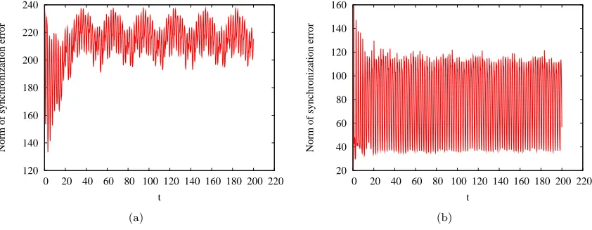
Figure 2. Network of three systems of generalized FHN type. The norm of synchronization
error given by the definition 2.3 on the interval of time [0,200] for the coupling strength α2=
α3= 0.3 : (a) between S1andS2, (b) betweenS2 andS3.
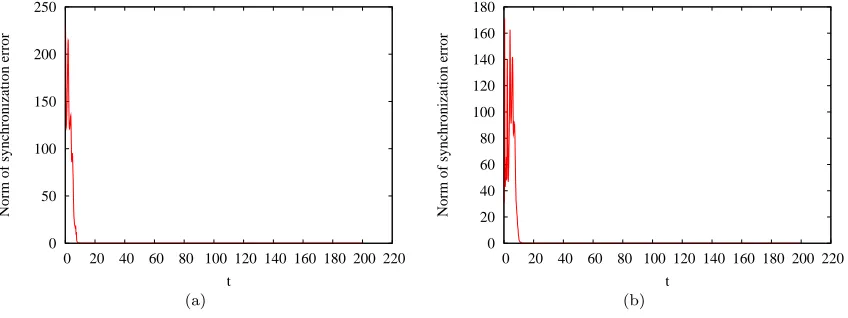
Our numerical simulations, see figure 1, 2, 3, 4, show that system (11) synchronize for a coupling strengthα2=α3
belonging to the interval [0.3,0.4]. In these figures, the initial conditions are (u1(x,0), v1(x,0)), particular
functions leading to multiple spiral pattern formation, see [8,9], and (u2(x,0), v2(x,0)) = (u3(x,0), v3(x,0)) = 1.
0 10 20 30 40 50 60 70 80 90 100 x1
0 10 20 30 40 50 60 70 80 90 100
x2
-2 -1.5 -1 -0.5 0 0.5 1 1.5 2
(a)
0 10 20 30 40 50 60 70 80 90 100 x1
0 10 20 30 40 50 60 70 80 90 100
x2
-2 -1.5 -1 -0.5 0 0.5 1 1.5 2
(b)
0 10 20 30 40 50 60 70 80 90 100 x1
0 10 20 30 40 50 60 70 80 90 100
x2
-2 -1.5 -1 -0.5 0 0.5 1 1.5 2
(c)
Figure 3. Network of three systems of generalized FHN type. Isovalues, of (a)u1(x, t),
(b)u2(x, t), (c)u3(x, t) at fixed time t= 190 for the coupling strengthα2=α3= 0.4.
0 50 100 150 200 250
0 20 40 60 80 100 120 140 160 180 200 220
Norm of synchronization error
t
(a)
0 20 40 60 80 100 120 140 160 180
0 20 40 60 80 100 120 140 160 180 200 220
Norm of synchronization error
t
(b)
Figure 4. Network of three systems of generalized FHN type. The norm of synchronization
error given by the definition 2.3 on the interval of time [0,200] for the coupling strength α2=
References
[1] E. M. Izhikevich, Dynamical systems in Neuroscience, The MIT Press, 2007. [2] J. P. Keener and J. Sneyd, Mathematical Physiology, Springer, 2009. [3] J.D. Murray, Mathematical Biology, Springer, 2010.
[4] R. A. FitzHugh, Impulses and physiological states in theoretical models of nerve membrane, Biophys. J. 1, (1961) 445-466. [5] A.L. Hodgkin and A.F. Huxley, A quantitative description of membrane current and its application to conduction and excitation
in nerve, J. Physiol. 117, (1952) 500-544.
[6] M. Marion, Finite-Dimensionnal attractors associated with partly dissipative reaction-diffusion systems, SIAM J. Math. Anal. 20 (1989) 816-844.
[7] Nagumo J., Arimoto S. and Yoshizawa S, An active pulse transmission line simulating nerve axon, Proc. IRE. 50 (1962) 2061-2070.
[8] B. Ambrosio, Wave propagation in excitable media : numerical simulations and analytical study, in french. Ph.D Thesis, University Paris VI, 2009.
[9] B. Ambrosio and M.A. Aziz-Alaoui, Synchronization and control of coupled reaction-diffusion systems of the FitzHugh-Nagumo type, CAMWA. 64 (2012) 934,943.