The Development of Maximum Likelihood Estimation Approaches for Adaptive Estimation of Free Speed and Critical Density in Vehicle Freeways

٭

The Development of Maximum Likelihood Estimation

Approaches for Adaptive Estimation of Free Speed and

Critical Density in Vehicle Freeways

A. Ramezani

1٭

, B. Moshiri

2

, A. Rahimi Kian

3

1- Assistant Professor, Control and Intelligent Processing Center of Excellence, School of ELec & Comp, Engineering, University of Tehran, Tehran, Iran

2- Professor, Control and Intelligent Processing Center of Excellence, School of ELec, & Comp. Engineering, University of Tehran, Tehran, Iran

3- Associate Professor, Control and Intelligent Processing Center of Excellence, School of ELec & Comp, Engineering, University of Tehran, Tehran, Iran

A

BSTRACT

The performance of many traffic control strategies depends on how much the traffic flow models are

accurately calibrated. One of the most applicable traffic flow model in traffic control and management is

LWR or METANET model. Practically, key parameters in LWR model, including free flow speed and

critical density, are parameterized using flow and speed measurements gathered by inductive loop detectors

and Closed-Circuit TV. The challenging problem here is continuous changes in these parameters due to

traffic conditions (traffic composition, incidents) and environmental factors (dense fog, strong wind, snow)

and missing data. In this paper Maximum Likelihood approaches are developed to the LWR model

identification while inaccurate observations are available at the traffic control center. A Maximum

Likelihood method is accomplished via the employment of an Expectation Maximization algorithm. To

approximate first and second derivatives of optimal filter without sticking in analytical complexities, The

EM algorithm is implemented based on particle filters and smoothers. Two convincing simulation results for

two sets of field traffic data are used to demonstrate the effectiveness of the proposed approaches.

K

EYWORDS

1-INTRODUCTION:TRAFFIC FLOW MODEL AND

PROBLEM STATEMENT

Many of traffic control systems are based on the use of a second-order macroscopic traffic flow model or LWR model [1], [2]. For a freeway which divided into N segments, discrete time state space LWR model is represented as:





 

 

   

k

s

k

 

k

r

k

q

k

q

T

k

k

i i i i i i i i i 

























_

]

[

)

(

1

₁ (1)









 

  



 



 





 

 

 



   

 

 

k

k k k v k r T k k k k vT k v v k v T k v k V T v k v v i i i i i i i i i i i i i i i i k i





















               

1 1

1 (2)

 

   

q

i i i i

i

k

k

v

k

q











(3)

 

k

   

k

q

k

s

_i





_{i i1} (4)

 

































a cr f

a

v

V







exp

1

(5)

In the above T is Time step size (hours) and ) ( ), ( ), ( ), ( ), ( ,

, i i k vi k qi k ri k si k

i





 are length, number,

mean speed (km/h), traffic density (veh/km/lane), traffic flow (veh/h), on-ramp inflow and off-ramp outflow of segment i at time kT, respectively. Also τ,υ,δ,κ are model

parameters which have the same values for all segments, and _i(k) is exiting rates on off ramp of segment i at time kT. The model characteristics are most sensitive to variations of the three other parameters denoted by  in the stationary speed equation (i.e., equation 5) which are usually unknown and depend on the physical infrastructure [3]. Usually this model has to be calibrated as exact as possible regarding to infrastructures and environmental condition of each physical site to have better performance and optimal use of infrastructures in traffic mobility. So, we need to develop available approaches to a better estimation of key traffic parameters including the free flow speed,

v

_f, the critical density,



_cr and the exponent α. As we usually have uncertainties and imperfectness in the traffic data set due to weather condition (rain, snow, fog and pollution) and link loss between sensors, here we develop statistical approaches to optimize the estimation results. Approaches used here are based on Maximum Likelihood (ML) parameter estimation accomplished via the employment of direct particle filtering and also via the employment of an Expectation Maximization (EM) algorithm. There is a little work which covers exactly the statistical estimation methods in traffic state estimation. The previous studies usually include classical estimation methods such as

filtering methods (Extended Kalman Filters, Particle Filters) or regression models (Least Square Error Methods). Finding a proper ML estimation can help traffic user to interpolate missing data or nearest possibility to control or predict congestion or recurrent traffic phenomenon. In the first part of this paper, regarding to a given LWR model and using maximum likelihood estimation including a direct particle filtering routine, the traffic flow model parameters referred to by

n R 



are estimated based on the input and output observations and information gathered by geographically distributed loop detectors implemented in the on-ramp, off-ramp, cross section and some pre-determined places in the urban roads and traffic infrastructure. In the second part of this paper, an Expectation Maximization (EM) algorithm is used to solve the maximum likelihood problem. Here an offline and online parameter estimation using the EM algorithm is addressed for Gaussian nonlinear LWR traffic flow model.

The rest of the paper is organized as follows: In Section 2, we describe the Maximum Likelihood estimation in a recursive and a batch manner. Section 3 presents maximum likelihood estimation based on expectation maximization algorithm and sequential Monte Carlo approach. Online EM algorithm using Split-Data Likelihood concept is reviewed in section 4. Test results of the algorithm by field data are shown in section 5. Finally in Section 6, we discuss the results and provide some concluding remarks.

2-RECURSIVE AND BATCH MAXIMUM LIKELIHOOD

ML estimation is a nonlinear system identification problem [4] seeking an estimate of the parameter values

n

R





ˆ

as

_:

)

,...,

(

arg

ˆ

1

y

N

y

p

MAX

_







 (6)

where

p

_

(

y

₁

,...,

y

_N

)

denotes the joint likelihood of N output measurements, as postulated by model output equation. In ML estimation methods, we seek



*based on

 

Y

_{n n0}

.

There are various earlier attempts in the literature [5] to solve the ML estimation problem based on particle filters. However, it still remains a challenging problem. Particle filter algorithm here used sequence of marginal distributions



p

_



x

_n

|

y

_0:n





to approximate the filter derivatives. Then a gradient ascent algorithm should be implemented to maximize likelihood function and compute the maximum likelihood estimates of the model parameters. Scaling the gradient components is based on estimates of the derivatives of the filter extracted via particle methods. The expression maximized in a standard Recursive ML (RML) estimation approach at iteration k

is a summation of log-likelihood functions

 

 





_







k

n n n

k

p

Y

Y

Y

p

0: ₀

log

|

0: 1

log

 

The expression p



Yn|Y_0:n₁



is known as the predictive

likelihood and can be written as [6]:







_{n n}



_{n n}

n n n n n

dx

Y

x

p

x

x

f

x

Y

g

Y

Y

p

: 1 1 : 0 1 1 1 : 0

|

)

|

(

)

|

(

|

    





    (7)

Maximization is performed by updating parameter estimate at time n using a Stochastic Approximation (SA) algorithm formulated by the following recursion [7]:

)

|

(

log

₁

1 0: 1 











_{n n n n}

n





p

n

Y

Y



(8)

where



_n1 is the parameter estimate at time

n



1

and

)

|

(

log

₁ 1 :

0 



p

n

Y

n

Y

n denotes the gradient of

)

|

(

log

₁ 1 :

0

Y

n

Y

n

p

n



.

This recursion needs a numerical

approximation from the expressions for

p





x

_n

|

Y

_0:n



and



x

n

Y

n



p



|

0:



starting from the recursion given below for the joint posterior density, we can derive the suitable formulation for the required gradient and Hessian matrix [8]:





), | ( ) , | ( ) | ( ) , ( | 1 : 0 1 : 0 1 1 : 0 : 1 : 0 : 0     

 n n n n n

n n n n n n n Y x p x Y x q Y Y p Y x Y x p     



(9)

One can improve Hessian matrix according to a recursive sample mean formulation such as [9]:

)

ˆ

(

1

1

1 1  









_{n n n}

n

H

H

n

H

H

(10) where:

)

|

(

ˆ

log

ˆ

1 : 0 2 





n n

n

p

Y

Y

H

_

Hessian matrix is invertible according to its properties- see [9] and [10] for details- and The Newton-type SA version of (8) is in the form of [10]:

)

|

(

ˆ

log

_{0: 1}

1

1 0: 1 









_



n n n n n

n

Y

Y

p

H

n 







(11)

An offline type of Maximum Likelihood Estimation algorithm, namely BML, can be used when a batch or a set observations

Y

0:_n is received in each time step. BML maximizes the log-likelihood logp(Y0:n) using a modified Stochastic Approximation recursion at iteration

m given by:

)

(

ˆ

log

_0:

1 m 1 n

m

m













p

m

Y



(12)

To do so, one can modify RML as follows: considering the parameter fixed at the current estimated value



_m1 , one runs RML during time step 0 to n and finally,

log

ˆ

(

_0:

)

1

Y

n

p

m



_ can be computed using a Monte Carlo method as:

)

(

ˆ

log

p

_m1

Y

_0:n



_









 _    





  n k N j j k N j j k n

k k k

k k

a

Y

Y

p

Y

Y

p

m m 0 1 ) ( 1 ) (

0 0: 1

1 : 0

)

|

(

ˆ

)

|

(

ˆ

1 1



 

Where

Y

_0:1





3-EM-BASED MAXIMUM LIKELIHOOD PARAMETER

ESTIMATION

The iterative gradient-based search procedures in MLE requires calculations of the likelihood and the predictor gradient, which in turn requires the solution of a nonlinear filtering problem as shown in [11]. In non-differentiable case (or in case it is non-trivial to extract), Expectation Maximization (EM) methods are considered as a well-known alternative for maximization of likelihood functions. Relaxation from computation of gradients is one of the remarkable advantages of EM method. Also this approach is well recognized as being particularly robust against trapping into local minima [12]. Getting the benefits of above comments, here an EM-based Maximum Likelihood estimation approach is developed for handling the LWR model calibration. The Expectation Maximization (EM) algorithm introduced in [13] demonstrates a non gradient-based approach to estimate the maximum likelihood postulated by (6) in a finite number of iterations. By introducing an extra data set, in applied statistics referred to as incomplete data or

missing data,X_n, the EM approach extends (6) as given below such that the solution of new problem be straightforward. So the key parameter to design a suitable EM problem structure is the choice of missing data [14]:

)

,

(

max

arg

)

,

(

ˆ

N N N

N

Y

p

X

Y

X

_







Using Bayes’ rule for conditional probability and taking logarithm leads to [14]:

) / ( log ) , ( log ) (

logp_ Y_N  p_ X_N Y_N  p_ X_N Y_N

Given observation Y_N setting  to a value ′ , taking conditional expectations of both sides of this equation with respect to , we obtain[14]:

                      ) , ( ) , ( } | ) / ( {log } | ) , ( {log ) (                v N N N Q N N

N Y Y E p X Y Y

X p E L

E-Step: Form the expected value of

L



(

X

,

Y

)

over the missing data X based on the current parameter estimate

k



and the measurements Y via [15]:











dX

Y

X

p

Y

X

L

Y

Y

X

L

E

Q

k

(

|

)

)

,

(

}

|

)

,

(

{

)

,

(

   





(13)

M-Step: Obtain a new estimate



_k1 by maximizing

)

,

(







Q

over  , i.e.:

) , ( max arg 1 k

k Q 







Iterating between these expectation and maximization steps is known as the Expectation Maximization (EM) algorithm [14]. Clearly, its employment requires a mechanism for computing the expectation involved in

) ,

( k

Q





, and also a means for maximizing Q(



,



k) over . Here, Sequential Monte Carlo methods (also known as particle filter) has been employed to approximate the distribution p (X|Y)

k

 in (13). With this

software available, then we can maximize

Q

ˆ

using any practical gradient-based search procedure. Here, the Sequential Monte Carlo is presented to calculate the

weights () |

~

i N t

q

and the smoothed particles

x

_t(_|i_N) .

4-TEST ON FIELD DATA

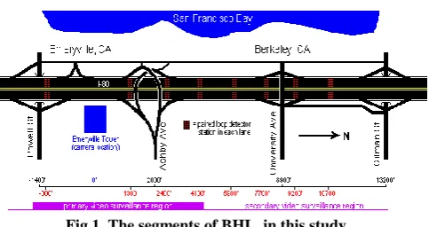
Berkley Highway Laboratory: The field data used first is from the Berkeley Highway Laboratory. A schematic of BHL is shown in Figure 1. The data chosen in this study are from Westbound, station 3, lane 3. Speed and flow measurements from the dual loop detectors were aggregated and converted to a 15 second speed and density data for one day (24 hour) in August 2003 [16]. Data has been selected such that it includes both free flow states and congested states. The initial parameter estimates were selected as:

, 100 ) 0 (

h km

v_f 

lane

km

veh

cr

(

0

)



20

/

/



5 . 1 ) 0

( 

a

]

,

,

[

v

_f



_cr

a







d

i

i

N

q

v

,



,





~

(

₀

,

1

),

.

.



The RML algorithm was implemented using the optimal importance density:

)

|

(

)

|

(

)

,

|

(

x

_n

Y

_n

x

_n1



g

Y

_n

x

_n

f

x

_n

x

_n1

q

_{  }

and N=1000 particles. The analytical and numerical values of the score vector

)

|

(

log

_0:1



p



Y

_n

Y

_n and the Hessian matrix )

| (

log 0: 1

2



 p Yn Yn were compared up to n=10000.

These were almost indistinguishable. An example of the comparison results obtained for the component

2 1 : 0 2

) | ( log

 



 p Yn Y n is shown in

Figure 2.

Fig.1. The segments of BHL, in this study

As it can be seen for the results in Figure 2, the estimate converged to a value



ˆ

in the neighborhood of the true parameter. We then applied the BML method to the traffic flow parameters. The parameter estimates for M=1000 iterations using N=1000 particles are shown in Figure 3. Our results are consistent with those obtained by approaches in [1].

(a)

0 100 200 300 400 500 600 700 800 900 1000 -120

-100 -80 -60 -40 -20 0

O

pt

im

a

l

Fi

lt

e

r

D

e

ri

v

a

ti

v

e

sample

0 5 10 15 20

80 100 120 140 160 180 200

vf

(

k

m

/h)

Fig. 2. (a) Analytical and numerical results for second derivative using N= 1000 (b)-(c)-(d) Estimation results for RML and BML: solid line: Sequence of RML parameter estimates for [v_f,_cr,a] and N=1000. Sequence of BML parameter estimates for [v_f,_cr,a] and N=1000

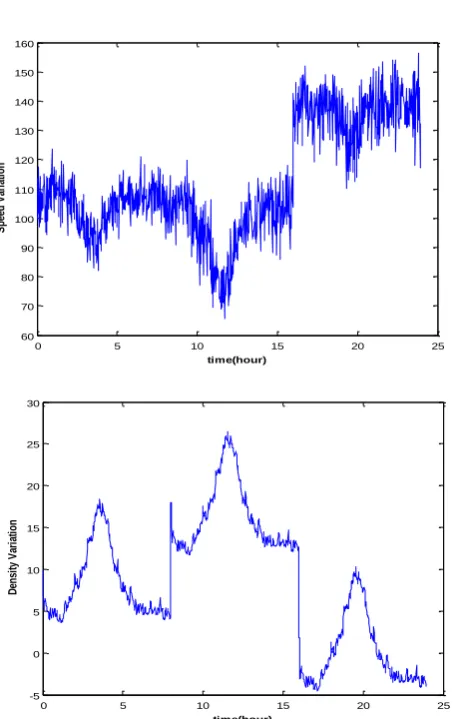
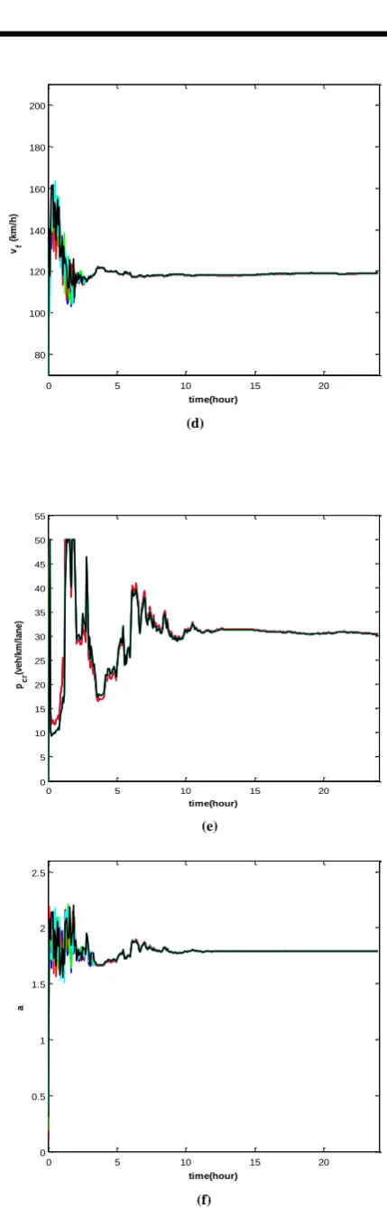
Parameter tracking: A unique advantage of the RML algorithm is its ability to track variations in. An example of the tracking performance of the RML algorithm based on the state space traffic flow model, having time-varying drift parameters, is shown in Figure 3 and 4. For the same data set, the EM Algorithm has been used with M=50 particles. Figure 3 shows the filtered estimated free flow speed, critical density and the exponent, respectively. Different initial values of the parameters were also used in the estimation. Results show that the estimation algorithm was not sensitive to these factors. It took about 5 hours for the estimates to settle at the steady state values.

Fig. 3. Data flow in a time varying parameter environment

0 5 10 15 20

0 5 10 15 20 25 30 35 40 45 50 55

pc

r

(v

e

h/

k

m

/l

a

ne

)

time(hour)

0 5 10 15 20

0 0.5 1 1.5 2 2.5

a

time(hour)

0 5 10 15 20 25

60 70 80 90 100 110 120 130 140 150 160

S

pe

ed

V

ar

ia

ti

on

time(hour)

0 5 10 15 20 25

-5 0 5 10 15 20 25 30

D

ens

it

y

V

ar

ia

ti

on

time(hour)

0 5 10 15 20

0 0.5 1 1.5 2 2.5

a

Fig. 4. (a)-(b)-(c): RML algorithm tracking performance for time-varying parameters using N = 1000 particles. (d)-(e)-(f): Estimated parameters: Estimated free flow speed, Estimated critical density and Estimated exponent, respectively.

2) Metro Freeway (Twin Cities Freeway): Another test field data was chosen from Minnesota freeway network, I-494 highway, between TH101 Boulevard to TH95 Street, Westbound (red light in Fig. 5). Speed and flow measurements from the 14 loop detectors, between detectors number 702 and 708 were aggregated and converted to 30 second speed and density data for 25 hours in February 2009 (Fig 5). The initial parameter estimates were selected as:

,

100

)

0

(

h

km

v

_f



lane

km

veh

cr

(

0

)



10

/

/



5

.

1

)

0

(



a

And EM Algorithm has been used with M = 100 particles. Figure 6 shows the filtered estimated free flow speed, critical density and the exponent, respectively. The steady state free flow speed is about 95 km/h, the steady state critical density is about 35 veh/km/lane and the mean exponent value is about 1.75.

0 5 10 15 20

0 5 10 15 20 25 30 35 40 45 50 55

pc

r

(v

eh/

km

/l

ane

)

time(hour)

0 5 10 15 20

0 0.5 1 1.5 2 2.5

a

time(hour)

0 5 10 15 20

80 100 120 140 160 180 200

vf

(

km

/h

)

time(hour)

0 5 10 15 20

0 5 10 15 20 25 30 35 40 45 50 55

pc

r(

ve

h/

km

/la

ne

)

time(hour)

0 5 10 15 20

0 0.5 1 1.5 2 2.5

a

(a)

(b)

(a)

(b)

(c(

(d)

(e)

(f)

Fig. 6. (a)Estimated free flow speed (b)Estimated critical density (c) Estimated exponent. (d)-(e)-(f) Parameter estimates for each of the simulation runs as they evolve over 1000 iterations of the EM method. The true parameter

0 5 10 15 20

70 80 90 100 110 120 130 140

v

f

(k

m

/h

)

time(hour)

0 5 10 15 20

0 5 10 15 20 25 30 35 40 45 50 55

p

c

r(

v

e

h

/k

m

/l

a

n

e

)

time(hour)

0 5 10 15 20

0 0.5 1 1.5 2 2.5

a

time(hour)

0 5 10 15 20

80 100 120 140 160 180 200

vf

(

k

m

/h)

time(hour)

0 5 10 15 20

0 5 10 15 20 25 30 35 40 45 50 55

pc

r

(v

eh/

km

/l

ane

)

time(hour)

0 5 10 15 20

0 0.5 1 1.5 2 2.5

a

values are

8 . 1 ) 0 ( , / / 30 ) 0 ( , 120 ) 0

(   veh km lanea 

h km

vf cr

To address the issue of finding appropriate initial parameter values and to illustrate the inherent robustness of the EM-based approach, each of the simulation runs was initialized at a randomly chosen initial estimate

)

0

(

f

v

which itself was formed using perturbations from

the true values. Using N=4000 data samples, and despite only using a very modest number of M=50 particles in the smoothing calculations, the empirical estimation results shown in Fig. 5 are encouraging. In particular, we should note that despite quite widely varying initializations, convergence to the true parameters occurred in most cases. Further simulations were conducted with M=100 and a higher number of particles, but without any significant performance benefit. This suggests a robustness of the EM-based approach to inaccuracies in computation in the E-step. In relation to this, note that the method requires ( 2)

NM

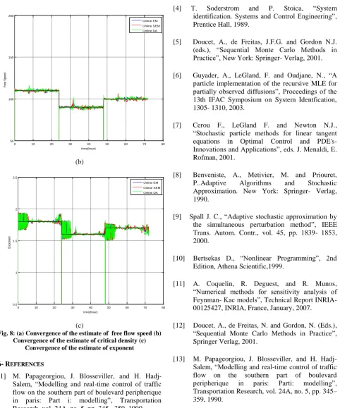
O floating point operations per iteration. The computational load is sensitive to the number of particles chosen, but scales well with increasing observed data length. To provide a reference point for these scaling comments, each simulation is required to present the Monte–Carlo presentation in Fig. 6 (d)-(f) completed within 3 minutes on a Pentium IV running at 3GHz. By way of comparison, alternative methods, including Newton-based gradient search were also tried, but proved very unsuccessful. Here, it is better to say these alternative methods: three different versions of gradient-based search Methods have been tried on the same platform, a Pentium IV running at 3GHz and the simulation for the same data base and initial condition completed in: 15 min (Quasi-Newton method ), 31 min (Gauss–Newton algorithm), 49 min (Gradient descent). The parameters estimated based on the data gathered in the first segment shown in Figure 7, However, It can be shown that other segment data produce near estimates with a little difference. In another word, the data generated by these parameters has less MSE in the first segment rather than other segments. But they can be accepted as an efficient estimates to provide data in another segment as illustrated in the Figure 7 for second segments. Apparently as we go far from the first segment the estimates will involve larger MSE. Finally, the Online EM algorithms were used for L =5 with a temperature _n0.5

n 

 . The data was chosen from three different highway traffic conditions from 3 days. Figure 8 shows the filtered estimates and the tracking performance can be easily seen.

(a)

(b)

(c)

0 5 10 15 20 25

100 105 110 115 120 125 130

E

s

ti

m

a

te

d

s

p

e

e

d

s

o

f

s

e

g

m

e

n

ts

Time(hour)

v-real v-estimation

0 5 10 15 20 25

1000 1500 2000 2500 3000 3500 4000 4500 5000 5500

E

s

ti

m

a

te

d

f

lo

w

s

o

f

s

e

g

m

e

n

ts

Time(hour)

q-real q-estimation

0 5 10 15 20 25

2 4 6 8 10 12 14 16

E

s

ti

m

a

te

d

D

e

n

s

it

ie

s

o

f

s

e

g

m

e

n

ts

Time(hour)

p-real

(d)

(e)

Fig.7. Real and Estimated data from the first segment (a) Speed ( 4.53*104)

MSE (b) Flow( 6.20*104)

MSE .

the second segment:(a) Speed (MSE6*104) (b) Flow

) 10 * 5 . 8

(  4

MSE (c)Density

5-CONCLUSION

In this study, several types of recursive estimators based on particle methods have been designed and tested to estimate the three important parameters of a second-order macroscopic traffic flow model. The particle methods to estimate the first and second derivative of the optimal filter in general state-space models have been presented. This allows the calculation of accurate approximations to the score vector and the Hessian matrix of the log-likelihood with respect to the model parameters. Based on this, a recursive and a batch algorithm to perform ML parameter estimation using a gradient ascent method were proposed. The Hessian

estimate can be used as an adaptive step-size in the gradient ascent recursion to provide faster convergence of the algorithm. The computational cost of the used particle methods for the filter derivatives is quadratic in the number of particles. Fast computation methods can however be employed to address this issue. Then, in this study, an offline Maximum Likelihood estimator based on EM algorithm has been presented whose key distinguishing features include the use of expectation maximization methods as opposed to more traditional gradient-based search and the use of Monte Carlo based “particle” methods for the computation of required smoothed state estimates, and a capacity for simply encompassing multivariable problems. Simulation results justified that it would probably benefit from an improved expectation step. The plug-and-play nature of the proposed EM algorithm implies that it is straightforward to use it with a different smoothing and maximizing algorithm and in any highway with different infrastructure. Finally, three online estimators based on EM algorithm and Split-Data Likelihood contrast function type have been provided to estimate time varying traffic parameters in different conditions and the invariant distribution of the missing data. These algorithms are simple and their effectiveness were demonstrated using two traffic field data.

(a)

0 5 10 15 20 25

1000 1500 2000 2500 3000 3500 4000 4500 5000 5500

E

s

ti

m

a

te

d

f

lo

w

s

o

f

s

e

g

m

e

n

ts

Time(hour)

q-real

q-estimation

0 5 10 15 20 25

100 105 110 115 120 125 130

E

s

ti

m

a

te

d

s

p

e

e

d

s

o

f

s

e

g

m

e

n

ts

Time(hour)

v-real

v-estimation

0 10 20 30 40 50 60 70 80

0 5 10 15 20 25 30 35 40 45 50 55

time(hour)

C

ri

ti

c

a

l

D

e

n

s

it

y

(b)

(c)

Fig. 8: (a) Convergence of the estimate of free flow speed (b) Convergence of the estimate of critical density (c)

Convergence of the estimate of exponent

6-REFERENCES

[1] M. Papageorgiou, J. Blosseviller, and H. Hadj-Salem, “Modelling and real-time control of traffic flow on the southern part of boulevard peripherique in paris: Part i: modelling”, Transportation Research, vol. 24A, no. 5, pp. 345– 359, 1990.

[2] Y. Wang, M. Papageorgiou, and A. Messmer, “A real-time freeway network traffic surveillance tool”, IEEE Trans. Control Systems Technology, vol. 14, no. 1, pp. 18– 32, 2006.

[3] L. Ljung., “System identification, Theory for the user. System sciences series”, Prentice Hall, Upper Saddle River, NJ, USA, second edition, 1999.

[4] T. Soderstrom and P. Stoica, “System identification. Systems and Control Engineering”, Prentice Hall, 1989.

[5] Doucet, A., de Freitas, J.F.G. and Gordon N.J. (eds.), “Sequential Monte Carlo Methods in Practice”, New York: Springer- Verlag, 2001.

[6] Guyader, A., LeGland, F. and Oudjane, N., “A particle implementation of the recursive MLE for partially observed diffusions”, Proceedings of the 13th IFAC Symposium on System Identfication, 1305- 1310, 2003.

[7] Cerou F., LeGland F. and Newton N.J., “Stochastic particle methods for linear tangent equations in Optimal Control and PDE's- Innovations and Applications”, eds. J. Menaldi, E. Rofman, 2001.

[8] Benveniste, A., Metivier, M. and Priouret, P..Adaptive Algorithms and Stochastic Approximation. New York: Springer- Verlag, 1990.

[9] Spall J. C., “Adaptive stochastic approximation by the simultaneous perturbation method”, IEEE Trans. Autom. Contr., vol. 45, pp. 1839- 1853, 2000.

[10] Bertsekas D., “Nonlinear Programming”, 2nd Edition, Athena Scientific,1999.

[11] A. Coquelin, R. Deguest, and R. Munos, “Numerical methods for sensitivity analysis of Feynman- Kac models”, Technical Report INRIA- 00125427, INRIA, France, January, 2007.

[12] Doucet, A., de Freitas, N. and Gordon, N. (Eds.), “Sequential Monte Carlo Methods in Practice”, Springer Verlag, 2001.

[13] M. Papageorgiou, J. Blosseviller, and H. Hadj-Salem, “Modelling and real-time control of traffic flow on the southern part of boulevard peripherique in paris: Parti: modelling”, Transportation Research, vol. 24A, no. 5, pp. 345– 359, 1990.

[14] Doucet, A. and Tadic, V.B., “Parameter estimation in general state-space models using particle methods”, Ann. Inst. Stat. Math., 55, 409- 422, 2003.

[15] N. J. Gordon, D. J. Salmond, and A. F. M. Smith., “Novel approach to nonlinear/non-Gaussian Bayesian state estimation”, In IEE Proceedings on

0 10 20 30 40 50 60 70 80

50 100 150 200

time(hour)

Fr

e

e

S

p

e

e

d

Online EM Online SEM Online DA

0 10 20 30 40 50 60 70 80

0.5 1 1.5 2 2.5

time(hour)

E

x

p

o

n

e

n

t

Radar and Signal Processing, volume 140, pages 107– 113, 1993.