Iranian Journal of Electrical & Electronic Engineering, Vol. 10, No. 3, Sep. 2014 223
Effects of Wind Speed Forecasting Error on Control
Performance Standard Index
S. M. Eslami*, H. Rajabi Mashhadi**(C.A) and H. Modir Shanechi***
Abstract: Increasing the penetration of wind turbine generations, needs more study about
controlling frequency impacts of power system. Frequency control is changed with unbalancing real-time system generation and load. Also wind turbine generations have more fluctuations and make system more unbalance. Then Automatic Generation Control (AGC) loop helps to adjust system frequency and the scheduled tie-line powers. The quality of AGC loop is measured by some indices. It is expected a proper measure shows the AGC performance just as it acts (operates). One of well-known measures in literature which was introduced by North American Electric Reliability Corporation (NERC) is Control Performance Standards (CPS). Previously it is claimed that a key factor in CPS index is
P K* /
σ . This paper focuses on impact of a day ahead wind speed forecast error on this
key factor and CPS. The study system is a two area system. One area has only thermal power and other area constitutes of significant wind farm and thermal power. Effects of wind speed standard deviation and also degree of wind farm penetration are analyzed and importance of mentioned factor criticised. After that, influence of mean speed forecast error on this factor is noticed.
Keywords: AGC, CPS, Load-Frequency Control, Wind Farm.
1 Introduction1
The main purpose of the electric power systems is to provide the customers’ demand with electricity, featuring high quality voltage and frequency. The errors in load forecasting and generation planning are the main factors results the frequency moving away from its permissible range and tie-line transmitted power deviating from the scheduled value. Generally, two approaches may be applied in order to solve afore-mentioned problem. The first approach is to improve load forecasting accuracy [1] and the second solution is to provide sufficient reserve power for the system.
However, technical limitations of generating units prevent the system from reaching desired frequency. Therefore, the frequency error is inevitable in the power systems. Thus, the AGC system tries to maintain power system frequency within permissible limits by adjusting
Iranian Journal of Electrical & Electronic Engineering, 2014. Paper first received 29 Aug. 2013 and in revised form 1 Feb. 2014. * The Author is with the Department of Electrical Engineering, Ferdowsi University of Mashhad, Mashhad, Iran.
** The Author is with the Department of Electrical Engineering at Ferdowsi University of Mashhad and the Center of Excellence on Soft Computing and Intelligent Information Processing, Ferdowsi University of Mashhad, Mashhad, Iran.
*** The Author is with Illinois Institute of Technology.
E-mails: [email protected], [email protected] and [email protected].
the system generation. To evaluate performance of the AGC, proper performance indices should be used. A suitable index should be able to reflect the actual quality of the AGC system.
Due to the accelerating penetration of the Wind Turbine Generators (WTGs) in recent years and future planning, the conventional indices must be reviewed and modified necessarily [2].
The indices are divided into two categories of deterministic and probabilistic. Owing to the uncertain nature of the WTGs in the power system and the large forecasting error of the wind power generation, the probabilistic indices seem to be more appropriate. The main goal of this paper is to study different statistical indices and evaluate AGC indices in power system which has large penetration of the WTGs.
Early studies on AGC were initiated in 1950. In a pioneering study by Cohn [3], the Area Control Error (ACE) was introduced as the error of the frequency control system, and the regulation has been analyzed based on different qualities of Economic Dispatch (ED) and AGC loop and then suitable state has been introduced. System frequency and tie-line power must be measured and then are used in frequency control loop. Besides, those measurements have errors. The influence of the measuring error in output of frequency control loop has been studied [4]. The requirements of
224 Iranian Journal of Electrical & Electronic Engineering, Vol. 10, No. 3, Sep. 2014
the AGC loop have been introduced in different items, one of these items is the significant differences between settling times of AGC, Load Frequency Control (LFC) and ED loops. Furthermore, the appropriate constant values for governor and recloser dead-bands have also been studied in [5]. The IEEE standard terms and definitions on AGC can be found in [6].
Later on, Control Performance Standards (CPS), the standard rules for frequency regulation service, including A1, A2, B1 and B2 rules were adopted by North American Electric Reliability Council (NERC). The A1 and A2 criteria were employed during normal conditions while B1 and B2 rules were applied during emergency conditions [7].
In an AGC system, the goal is to keep changes in tie-line power error (ΔPtie) and frequency error (ΔF) as small as possible. However, reaching this goal results in too much wear and tear in generating units [8]. Hence, the average value of the ACE signal is forced to zero, not instantaneous ACE. In fact, removal of a non-zero value from the averaged ACE signal requires changes in generation level and energy transfer between control areas. On the other hand, in 50 % of the control actions to bring the negative value of ACE to zero, a positive change in generation has had an inverse effect on ACE and vice versa [6].
Large rate of changes in ACE may require fast changes in the units' generations with its associated financial cost. Furthermore, large values of ACE result in large deviation in the units' generations. It is to be noted that repeatation rate and amplitude of changes are important, and ACE doesn’t reflect deviation speed. So ACE is not a good index for AGC. A good AGC index must be directly related to AGC quality [9].
In 1999, CPS1 and CPS2 indices were introduced by NERC. Compared with previous indices, there is less maneuvering and wear & tear in the units’ generation when these indices reach to accepted standard values. So system operation using NERC indices is more economic.
CPS1 and CPS2 are based on limiting the standard deviation of Δf, during different periods of time. The time-window for calculating the average values has a great impact on their results [9]. Short time-window used for average calculation reduces the effect of the idea of using the statistical information and is getting closer to calculations with online data. On the other hand, long time-window does not monitor deviations of the system. These indices have also been used as control signals in AGC (in replacement of ACE integral) [10].
It is proven that permitted values of error in CPS1, guarantees permitted value of CPS2 [11]. Indicator of Regulating Trajectory Tracking (IRTT) and Regulating Help Indicator (RHI) indices have also been defined by EDF [12]. Like CPS1 and CPS2, these indices are based on the average calculation of the product of the two terms. These two terms are functions of ΔPtie and ΔF (or ACE). There are some differences in the monitoring
of the system operation using CPS or RHI. In some situations, RHI index detects the system status as improper and identifies a need for emergency operations, while CPS rules detect the system situation as normal or correctable with normal control methods and does not require emergency operations.
On the other hand, from the viewpoint of the power generation regulation, fossil fuel generators have basic differences with WTGs. For instance, to regulate the power generation in a certain value, the fuel should be provided and the technical condition of the unit should be proper.
Although ambient temperature is one of the technical parameters of the generation units, it is possible to forecast it with a great accuracy for the next days [13]. Therefore, appropriate generation planning could be done for the next days if sufficient fuel is available. In this condition, the error of actual generation and planned generation will be very small. Although such a small error is not considerable, but accumulation of the small errors of the units or loads in the system will result in large frequency and tie-line power errors. This would be important for the system.
To decrease the frequency error of the system, units with fast maneuvering ability serve as the AGC units. These units can easily change their output in less time compared to other units. Since the generation of the WTGs is usually at their maximum power point, they cannot increase their generations to take part in the AGC. On the other hand, due to the large error in wind speed forecasting, power generation error of a WTG is much more than a conventional unit. Therefore, not only WTGs cannot operate in AGC, but also their presence in the system requires participation of more thermal units in the AGC.
Hence due to ever-increasing penetration of WTG, a crucial question arises: Are conventional control performances enough in power systems with large-scale wind power penetration? In this paper, we are going to find an answer to this question.
The rest of this paper is organized as follows. In section 2, a test system is explained and the relevant mathematical equations are presented. In section 3, probabilistic equations are defined. The zero-mean error in wind speed forecasting is discussed in subsection 3-1 and the non-zero mean condition is addressed in subsection 3-2. Finally, concluding remarks are presented in section 4.
2 Problem Description
In this paper, the test system consists of two control areas. Errors in generation planning and load forecasting have been considered for both control areas.
The system frequency error and tie-line power error is denoted by ∆f and ∆Ptie, respectively and Ki shows
the frequency response characteristic of the i-th control area. Unit of “f” and “∆f” is Hz. Units of P, ∆P, P1, P2,
∆R1, ∆R2, ∆G1, ∆G2, ∆L1, ∆L2 are MW. Units of K1, K2
Eslami et al: Effects of Wind Speed Forecasting Error on Control Performance Standard Index 225
and K are pu.MW/Hz. If the load forecasting error and generation planning error in area 1 are denoted by ∆L1
and ∆G1, respectively, then the overall error in load
forecasting and generation planning of the first area would be [14]:
1 1 1
R G L
Δ = Δ − Δ (1)
Hence:
1 2
( ) / ( * )
f R R K P
Δ = Δ + Δ (2)
where:
1 2
P = P + P (3)
1 1 2 2
( * * ) /
K = K P+K P P (4)
and
2 2 1 1 1 2
( * * * * ) / ( * ))
tie
P K P R K P R K P
Δ = Δ − Δ (5)
where, P1 and P2 are generation capacities of the two
control areas in Fig. 1.
Assuming ∆R2 = 0 we'll have:
) P * K /( P
f=Δ tie 2 2
Δ (6)
Therefore, according to Eq. (6), an increase in the power transmitted from the first area results on the frequency increase in the power system. It’s different of a general system. In general, we think that after increasing output power of an area or increasing loads of that area.
Therefore, according to Eq. (6), an increase in the power transmitted from the first area results on the frequency increase in the power system. It’s different of a general system. In general, we think that after increasing output power of an area or increasing loads of that area, frequency of that system must be decreased. So, the system operator in the first area detects this condition as unusual. On the other hand, the second area senses the frequency increase as a normal and expected response of the system, since the additional power is transmitted into this area through tie-line (although the second area does not need this power).
Considering ∆R1 = 0, we will have
) P * K /( P
f=−Δ tie 1 1
Δ (7)
In Fig. 2, the operating line with negative slope is related to Eq. (7). The behavior of the system in this condition is opposite to the system behavior associated
with positive-slope line. According to Eq. (7), increase in the transmitted power from the first control area decreases the frequency of power system, which is quite in the contrary to the system behavior associated with Eq. (6). However, if ∆R1 and ∆R2 are non-zero, then the
slope of the operation is the function of the parameters of these two control areas (K1, K2, P1, P2) and the load
disturbances (∆R1, ∆R2). This condition holds in the
power system during at all times.
Generally, if the operating point lies in quadrature 1 or 3, it means that control area 1 is the main source of disturbances, but if it lines in quadrature 2 or 4, the major part of the load disturbance happens in the control area 2. Probabilistic approaches have been used here to study these behaviors.
3 AGC Probabilistic Modeling
It's assumed in this paper that the first control area has significant WTG penetration. The wind speed forecast error has a non-zero mean and significantly large standard deviation. In proportion to the wind speed forecast error, is the difference between the planned generation and the actual generation. Hence, it's reasonable to say that the error in estimation of the WTGs generation has a non-zero mean and large standard deviation. The probability distribution of the load and generation error in the control areas have been considered as normal distribution:
) , ( N ) R (
PDF Δ 1 = μ1 σ1 (8)
) , ( N ) R (
PDF Δ 2 = μ2 σ2
Second area does not have any WTGs. Therefore, generation of this area has zero-mean error. Also the correlation between the generation and load planning errors of these two control areas is neglected and it is assumed that these parameters are independent. Hence, we'll have:
) R ( PDF * ) R ( PDF ) R , R (
PDF Δ 1Δ 2 = Δ 1 Δ 2 (9)
Since,
2
1 R
R R = Δ + Δ
Δ (10)
) , 0 ( N * ) , ( N ) R R R , R (
PDF Δ 1 Δ 2=Δ −Δ 1 = μ1 σ1 σ2 (11)
1 1
1 2
1 2 1
2
1 1
2 2
1 2
2 1
2 2 2
1 2 1
2 2 2 2
1 2 1 2
2
1
2 2 2
1 2 1
2 1
( exp
2
2 1 1
exp exp
2 2
2 1
exp 1
2
1
exp exp
2
( R μ ) PDF R , R)
π σ σ σ
( R R ) μ
π σ σ
σ σ
σ σ σ
ΔR ΔR
σ σ σ σ
μ ΔR
R
σ σ σ
⎡ Δ − ⎤
⎢ ⎥
Δ Δ = × − ×
× × ⎢⎣ ⎥⎦
⎡ Δ − Δ ⎤ ⎡ ⎤
⎢− ⎥= × ⎢− ⎥×
× ×
⎢ ⎥ ⎣ ⎦
⎣ ⎦
⎡ + ⎡⎛ ⎞ ⎤⎤
⎢− ×⎢⎜ − ⎟ ⎥⎥×
⎢ × ⎢⎝ + ⎠ ⎥⎥
⎢ ⎥
⎢ ⎣ ⎦⎥
⎣ ⎦
⎡ ⎤
− × ×Δ
⎢ + ⎥
⎣ ⎦ 1
⎡ ⎤
⎢ ⎥
⎣ ⎦
(12)
Fig. 1 schematic diagram of the test system.
226
Fig. 2 ∆Ptie–∆f
Five term term is indep constant valu µ1 and σ1. V
This term can µ1 and ∆R1 a
of ∆R1, ∆R, σ
∆R1 is a
cannot be m analyze the power flow based on the to whole sys
measured in a
density func and ∆f, instea P * K R = Δ 1 tie R P
Δ = Δ +
in Eq. (12), w
(
(
1 2 1 2 1 2 1 2 1 Δf μexp ΔPt
σ
σ σ
1 exp
2σ σ
K P 1 exp
2 σ
PDF( , ΔPti
⎡ × ⎢ ⎣ ⎡ + ⎢− ⎢ × ⎢⎣ ⎡ × ⎢− ⎢ ⎣ Analyzing different con 1 1 K P
K P σ
× −
×
Setting σ
deviation of ∆
P * K1 1
1 < σ
Therefore denoted by g
f Curve.
ms can be ide pendent of ∆R
ues of σ1 and
alues of µ1 an
n take large an are large. The
σ1 and σ2.
variable in measured by
probability o error, this pro parameters a stem. The err
all control are
ctions should
ad of∆R and ∆R f
* P Δ
1* *1 K P Δf
we'll have:
)
)
1 2 1 1 2 2 tie 2 2 2 2 1 2tie-K P Δf
σ
ΔP K P
σ
2 P Δf
exp
σ
ie
π σ σ
) = × × ⎤ × × ⎥ ⎦ ⎛ + × ⎜ ⎝ ⎤ × ⎥ × ⎥ + ⎦ ⎡ ⎢ ⎣
3.1 Zero
g the factor K nditions, if: 2 1 2 2 1 2 0 σ
σ +σ > σ12 + σ22 =
∆R, then Eq.
P * K
σ <
e, the param gi in the follo
Ir
entified in Eq
R and ∆R1 and
d σ2. Second t
nd ∆R1 appear
nd quite diffe remaining ter
the first con the second a f frequency e obability shou and signals wh
ror signals ∆P as. Therefore
be rephrased
R1. Substitutin
2 1 2 1 1 1 2 1 1 tie 1 2 1 μ 1 exp 2σ
K P σ
(
K P σ
μ
( P K
σ ⎡ ⎤ × ⎢− ⎥× ⎣ ⎦ ⎤ × ⎦ × × − ×
× Δ +
⎡ ⎣
o Mean Error
K*P*∆f in th
0
σ2
where σ (16) is restate
meter σi/ K
owing, plays a
ranian Journa
q. (12). The f only depends term is related
in the fifth te erent values w rms are functi
ntrol area wh area. In order error and tie-uld be expres hich are availa
Ptie and ∆f can
e, the probabi d to include ∆
ng: ( ( 2 1 2 2 1 2 σ ) f σ
P Δf)
×
⎤ ⎞ ⎥
Δ ⎟ ⎥×
+ ⎠ ⎥⎦
× × ⎤⎥
⎦
(
r
he fourth term
(
is the stand ed as:
(
i
i*P , which
an important r
al of Electrica
first s on d to erm. when ions hich r to line ssed able n be ility
∆Ptie
(13) (14) (15) m in (16) dard (17) is role in con tha roo sys dis fas lar and act con inc fre mo are red con hen 3 s val ∆f of axe qua bei sta Be the and opp wil pla inc the inc fou Fig
l & Electronic
determining ntours in diff at gi's unit is
ot of ∆f*∆P. W stem. An are sturb power sy ster and there
ge Pi means m
d its higher tions. Hence, ntrol area in capability of equency. An a ore disturbed ea with small ducing error ntribute to red Analyzing E nce, the secon shows contou lues of k = g1/
Based on Fig plane have di If gi for two
the ellipse ar es and the p adrants are eq ing in norma ate (quarters 1 esides, the pro e same. Howe d third quad posing behav ll restore the f The probabil ane is not the crease in g2 w
e first and thir crease the pr urth quadrants
g. 3 Contours of
c Engineering
the locatio ferent control
Hz *
MW whic
We named it ea with large ystem. Large e will be less more nominal
capability i we can interp n disturbing
maneuvering area with larg and can’t wor gi not only
due to its d duce error occ Eq. (15), first
nd and third te urs with same
/g2.
g. 3, even add ifferent probab
control areas re parallel to probabilities o
qual. In other al state (quart and 3) are th obability of p
ever, electrica drants of the
ior. In this ca frequency to it lity of being in same if gis ch
will increase t rd quadrants. H robability of s.
f constant PDF.
g, Vol. 10, No.
on of the areas. It sho ch is the unit as the ability er σi has mo
Ki makes AG
s frequency e l power of the in maneuveri pret gi as the
power syst g for contro ge gi can mak
rks well in A can maneuve disturbances,
urred by other consider the erms are equa e probabilities
odd quadrant bilities. s is the same,
the horizonta of being in r words, the p ters 2 and 4) he same for c
resence in all al control are e ∆Ptie-∆f pla
ase, the other ts nominal va n different qu hange. For a c the probability Hence a decre
being in the
.
3, Sep. 2014
constant-PDF ould be noted of the square of disturbing ore ability to GC operation error. Finally, e control area, ing in AGC ability of the tem and its olling system ke the system GC, while an er enough for but also can r areas.
case µ1 = 0;
al to one. Fig. s for different
ts of the ∆Ptie
-the diameters al and vertical each of four probability of or abnormal ontrol area 1. l quadrants is ea in the first ane observes r control area
lue.
uadrants of the onstant g1, an
y of being in ease in g2 will
e second and F d e g o n , , C e s m m n r n ; . t -s l r f l . s t s a e n n l d
Eslami et al:
If the fir system frequ
1- It's m probability d quadrants, s corrective ac 2- It sho small values Contrary small and h values of ∆P not appropria
A change the axis of s skewness of Therefore quarters wil being in the Density Func of the first co is shown in F For ident equal to 50 probability i defined simil H11 is the
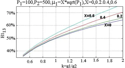
area in the f H13 and H14
the probabili the first an probability o second and f equal to unity
In Fig. 4 different va sensitivity o capacity in c If the initial additional 10 will increase installed cap 400 MW is increase abou So it can farm does no wind farm.
Fig. 4 H113 ve
Effects of Wi
rst control ar uency, then:
more appropr distribution b since such u ctions in the sy uld have larg of ∆R1.
to the previou has large valu Ptie and ∆f for
ate for this are e in g1 has sev
symmetry of t its curve will e, the probab ll change. Fo e first and th ction (CDF) f ontrol area in Fig. 4. tical values of 0 % while f increases. The
larly.
e probability o first quadrant
4 can be defin
ity of operatio d third quad of operation fourth quadra y.
4, H113 versu
alues of P1. f H113 to k i
control area 1 installed capa 0 MW is also
e about 3%. pacity in area also installe ut 2%. n be conclude
ot affect H113
ersus k, differen
ind Speed For
rea competes
riate that ma be in the sec units are mo
ystem. ge values of ∆
us condition, ues of σ1, it
small values ea and also oth
eral effects on the PDF chan also change. bility of bein or a better u hird quarters, for the probab
the first quad
f g1 and g2, t for larger va e parameter H
of operation o of the plane ed. Now, H11
on of the firs drant. Likewi of first con ants. Sum of H
us k = g1/g For small is also small
increases, the acity in area installed (k = . On the oth 1 is 100 MW ed (k = 1.8),
ed that installi
3 more than i
nt P1.
recasting Erro
s for controll
ajor part of cond and fou ore effective
∆Ptie and ∆f.
if the first are can sense la of ∆R1, whic
her areas. n PDF (∆f, ∆P nges and also
ng in the pl understanding the Cumulat bility of operat drant (called H
this probability alues of g1, H11 can also
of the first con . Similarly, H
13 = H11 + H1
st control area ise, H124 is
ntrol area in H124 and H11
g2 is plotted values of . If the insta en H113 will r
1 is 10 MW = 1.8), then H her hand if W and additio , then H113 w
ing a large w installing a sm
or on Control P
ling its urth for By ea is arge h is
Ptie):
the
lane g of
tive tion H11)
y is the o be
ntrol H12,
13 is
a in the the
13 is
for P1, lled rise. and H113 the onal will wind mall spe WT non wil be eff Fig abo me zer cha inc 100 (w on ide Th con sho AG con pro cha qua ma can val ma hig ope me ave win som sm lar dec Fig Performance 3.2 As mentione eed has a non TGs, the mea n-zero [15, 16 ll not coincide displaced. T fects on the v g. 5 show the For X = 0 ( out 63%. For ean error), H1 ro mean erro anges in H11
creasing the i 0 MW to 500 ith zero mean Hence wind AGC perform
Based on Fi entical gi for
herefore, gi is
ndition of the ould be defin GC in differen Fig. 6 shows nstant proba obability of op
anges, but a adrant decrea aximum error
n be said that lue for the m aximum value gher probabilit The curves eration in the ean of genera
erage of powe nd speed fore me effects on
It can be un mall values of ge change in crease the valu
g. 5 H113 versus
Standard Inde 2 Non-Zero
ed earlier, the n-zero mean. an error in ge 6]. In this case e with the cen These chang values of H11
effect of μ1 o (zero mean er r this value of
13 will be abou
or of the win
3. In addition
installed capa 0 MW leads to n error).
speed forecas mance than ins ig. 5, if μ1 is all areas, the not a proper e system. He ned for determ nt control area
s the effect of ability. In th
peration in th also the max ases and the in the third qu t in the condi mean error of e of error is
ty.
in Fig. 6 e first and thi ation and lo er error can b ecasting. This the performan nderstood from g1, having a n
the curve of H ue of H113, su
s k–different M
dex Mean Error
e error of est Therefore, in eneration plan e, the center o nter of coordin ges may hav
3 and H124. T
n H113.
rror) and k = f k and X =
ut 67 %. It me nd forecastin n, it was seen acity of a win
o only 3% inc
sting error ha stalling more w s non-zero an en H113 will n
index for de ence an appr mining the pe as.
f μ1 on the co his case, no he first and th ximum error
e absolute v uadrant increa ition of havin f generation a larger and h
show the p ird quadrants
ad error. Inc be due to the s error would nce of the AG m the above f non-zero μ1 w
H113. Therefor
ufficient amou
Mean1.
227
timating wind n presence of nning will be f the contours nates and will ve significant The curves in
= 1.8, H113 is
0.4 (non-zero eans that non-ng forces 4% n before that nd farm from crease in H113
as more effect wind farms. nd there is an
not be 50 %. termining the opriate index erformance of
ontours of the ot only the hird quadrants in the first value of the ases. Hence, it ng a non-zero and load, the happens with
percentage of for non-zero crease in the large error in d surely have GC.
figure that for would cause a re, in order to unt of reserve
7 d f e s l t n s o -% t m 3 t n . e x f e e s t e t o e h f o e n e r a o
228
should be c frequency er operation an AGC.
4 Conclusio
The high considerably required to r In this pape forecasting h is non-zero WTGs. For mean error i control area responsible f it. Furthermo
P K*
σ , w
good index efficient deci a unit or c Therefore, performance should be de
Finally, i forecasting e installing m installing sm than installin define new a
Appendix
The nome
AGC A
WTG W
CPS C
ACE A
LFC L
NERC N
C
ED E
IRTT I
RHI R
Fig. 6 Countor
considered fo rror and tie-lin nd hence to av
on
h penetration y affect the po e-assess conv er, it was as has non-zero m
mean genera a system wi in wind spee has a large for this big er ore, it was sho which had bee and used in ision criterion control area
better indic in the presen fined. it was found error has mo more wind f mall wind farm ng large win and better inde
enclature is as Automatic Gen Wind Turbine Control Perfor Area Control E Load Frequenc North Ame Corporation Economic Dis Indicator of Re Regulating He
rs with non-zer
Ir
or WTG to ne power flow void poor per
n of bulk w ower system a ventional perfo ssumed that mean error an ation error in
ith small WT d forecast, th effect on the rror which AG own in this pap en previously n CPS1 & C n to assess the in load fre ces for mo nce of large W
in this paper ore effects on farms. As a ms has more in d farms. We ex in next rese
s follows: neration Cont Generator rmance Standa Error cy Control erican Elect patch egulating Traj elp Indicator
ro μ1.
ranian Journa
prevent a la w in the time rformance of
wind farms m and therefore ormance index the wind sp nd therefore th the presence TG and non-z he correspond e AGC. WTG GC must rem per that the in y introduced a CPS2, is not
e effectivenes equency cont onitoring A WTG penetrat
that wind sp n the AGC t another findi nfluence on A are working earches. trol ard tric Reliabi jectory Tracki
al of Electrica
arge e of the may it's xes. peed here e of zero ding G is move ndex as a an s of trol. AGC tion peed than ing, AGC g to ility ing Re [1] [2] [3] [4] [5] [6] [7] [8] [9] [10 [11 [12
l & Electronic eferences
] L. Ghods
Long-Term Comprehe
Electrical
4, pp. 249
] P. E. McS
“Probabili timing o
Transactio
pp.
1166-] N. Cohn,
Interconne
Power Ap
12, pp. 15
] L. A.
“Interrelat Deviation Interconne
Power Ap
2, pp. 520
] C. Conco
Control C Performan
Apparatus
752-756, M
] “IEEE S
Automatic Systems”,
Apparatus
1364, 199
] M. Yao, R
Based on Standard
IEEE Tra
No. 2, pp.
] Y. Wan a
Impact on
Report, N
] N. Jaleeli
Control
Transactio
pp. 1092-0] Real Pow
NERC
ftp://www /BAL-001
1] G. Gross
Frequency Criteria”, Vol. 16, N
2] N. Mauej
Dupuis an Frequency Between IEEE Tra pp. 1382-c Engineering
and M. Kalan m Electric Lo ensive Revie
l & Electronic
9-259, Dec. 20 Sharry, S. Bo istic forecast of peak ele
ons On Powe
1172, May 20 “Considerati ected Areas”
pparatus and S
527-1538, Dec Mollman tionship of n, and Ina
ected System
pparatus and S
0-525, Feb. 19 ordia, “Effect Characteristics
nce”, IEEE s and Systems
May 1969. Standard De
c Generation , IEEE T s and Systems
92.
R. R. Shoults n NERC's N and Disturb
ansaction on
. 852-857, Ma and J. R. Liao
n WFEC Syst
NREL, TP-500 i and L. S.
Performanc
ons on Power
1099, Aug 19
wer Balancin Standard
w.nerc.com/pu 1-0.pdf, 2005. and J. W. y Control
IEEE Transa
No. 3, pp. 520-ouls, T. Marg nd J. M. Tesse
y Control Sys American an
ans. on Power
1387, Nov. 20
g, Vol. 10, No.
ntar, “Differen oad Demand F
ew”, Iranian c Engineering
011.
ouwman and G ts of the ma ectricity dem
er Systems, Vo 005.
ions in the R ”, IEEE Tra
Systems, Vol. c. 1967.
and T. Time Error advertent Flo m”, IEEE Tra
Systems, Vol. 968.
t of Prime-M on Electric P
Transactions s, Vol. PAS-8 efinitions of
Control on E
Transactions s, PAS-89, No
and R. Kelm, New Control
bance Contro
Power Syste
ay 2000. o, Analysis of
tem Operation
0-37851, Aug VanSlyck, “ ce Standar
r Systems, Vo 99.
ng Control P BAL-001-0
ub/sys/all_upd
Lee, “Analy Performance
actions on Po
-525, Aug 200 gotin, M. Tro eron, “Measur stem Service: nd European
r Systems, Vo 000.
3, Sep. 2014
nt Methods of Forecasting; A
Journal of g, Vol. 7, No. G. Bloemhof, agnitude and
mand”, IEEE
ol. 20, No. 2,
Regulation of
nsactions on
PAS-86, No.
Kennedy, r, Frequency ow on an
ansactions on
PAS-87, No.
Mover Speed Power System
s on Power
88, No. 5, pp.
Terms for Electric Power
on Power
o. 6,
“AGC Logic Performance ol Standard”,
ems, Vol. 15,
f Wind Energy ns, Technical 2005. “Nerc’s New
rds”, IEEE
ol. 14, No. 3,
Performance,
0, online:
dl/standards/rs
ysis of Load Assessment
ower Systems, 01.
otignon, P. L. rment of Load : Comparison n Indicators”, ol. 15, No. 4, f A f . , d E , f n . , y n n . d m r . r r r -c e , , y l w E , : d t , . d n , ,
Eslami et al: Effects of Wind Speed Forecasting Error on Control Performance Standard Index 229
[13] A. Khotanzad, M. H. Davis, A. Abaye and D. J. Maratukulam, “An artificial neural network hourly temperature forecaster with applications in
load forecasting”, IEEE Trans. on Power
Systems, Vol. 11, No. 2, pp. 870-876, May 1996.
[14] T. Sasaki and K. Enomoto, “Statistical and
Dynamic Analysis of Generation Control
Performance Standards”, IEEE Transaction on
Power Systems, Vol. 22, No. 4, pp. 476-481, May 2002.
[15] EPRI, California Regional Wind Energy
Forecasting System Development, Vol. 1, Exclusive Summary, EPRI, CEC-500-2006-089, Sep 2006.
[16] C. P. Sweeney P. Lynch and P. Nolan, “Reducing errors of wind speed forecasts by an optimal combination of post processing methods”,
Meterological Applications, Vol. 20, No. 1, pp. 32-40, March 2013.
Sayyed Mahdi Eslami was born in Mashhad, Iran, in 1966. He received the B.Sc. and M.Sc. degrees both from the Department of Electrical Engineering of Sharif University of Technology, Tehran, Iran in electrical power system engineering. He is studying for Ph.D. degree in the Ferdowsi University of Mashhad, Iran. His research interests are wind farm operation, power electronics and drives.
Habib Rajabi Mashhadi was born in Mashhad, Iran, in 1967. He received the B.Sc. and M.Sc. degrees with honor from the Ferdowsi University of Mashhad, both in electrical engineering, and the Ph.D. degree from the Department of Electrical and Computer Engineering of Tehran University, Tehran, Iran, under joint cooperation of Aachen University of Technology, Germany, in 2002. He is as Professor of electrical engineering in Ferdowsi University of Mashhad and is with the Center of Excellence on Soft Computing and Intelligent Information Processing, Ferdowsi University of Mashhad, Mashhad, Iran. His research interests are power system operation and planning, power system economics, and biological computation.
Hassan Modir Shanechi, Senior Member IEEE, obtained his M.Sc. in Electrical Engineering with Distinction from Tehran University and his Ph.D. in System Science from Michigan State University. He was with the EE Department of Ferdowsi University, Mashhad, Iran and also an associate professor at the Department of Electrical Engineering, New Mexico Tech 2001-04. He joined the Electrical and Computer Engineering Department at Illinois Institute of Technology in August 2007. His general area of research is nonlinear and intelligent systems. He has been especially active in the area of power system dynamics and security. His research interests include power system operation, economics, and dynamics, large scale and intelligent systems, and distributed energy resources.