www.geosci-model-dev.net/10/1467/2017/ doi:10.5194/gmd-10-1467-2017
© Author(s) 2017. CC Attribution 3.0 License.
ASIS v1.0: an adaptive solver for the simulation of
atmospheric chemistry
Daniel Cariolle1,2, Philippe Moinat1, Hubert Teyssèdre3,†, Luc Giraud4, Béatrice Josse3, and Franck Lefèvre5
1Climat, Environnement, Couplages et Incertitudes, UMR5318 CNRS/Cerfacs, Toulouse, France 2Météo-France, Toulouse, France
3Centre National de Recherches Météorologiques, UMR3589 CNRS/Météo-France, Toulouse, France 4Institut National de Recherche en Informatique et en Automatique, Talence, France
5Laboratoire Atmosphères, Milieux, Observations Spatiales, CNRS/UPMC/UVSQ, Paris, France †deceased, April 2013
Correspondence to:Daniel Cariolle ([email protected]) Received: 9 November 2016 – Discussion started: 21 November 2016
Revised: 9 March 2017 – Accepted: 16 March 2017 – Published: 11 April 2017
Abstract. This article reports on the development and tests of the adaptive semi-implicit scheme (ASIS) solver for the simulation of atmospheric chemistry. To solve the ordinary differential equation systems associated with the time evo-lution of the species concentrations, ASIS adopts a one-step linearized implicit scheme with specific treatments of the Ja-cobian of the chemical fluxes. It conserves mass and has a time-stepping module to control the accuracy of the numeri-cal solution. In idealized box-model simulations, ASIS gives results similar to the higher-order implicit schemes derived from the Rosenbrock’s and Gear’s methods and requires less computation and run time at the moderate precision re-quired for atmospheric applications. When implemented in the MOCAGE chemical transport model and the Laboratoire de Météorologie Dynamique Mars general circulation model, the ASIS solver performs well and reveals weaknesses and limitations of the original semi-implicit solvers used by these two models. ASIS can be easily adapted to various chemical schemes and further developments are foreseen to increase its computational efficiency, and to include the computation of the concentrations of the species in aqueous-phase in ad-dition to gas-phase chemistry.
1 Introduction
In chemical transport models (CTMs) or general circula-tion models (GCMs), the descripcircula-tion of atmospheric chem-istry has rapidly increased in complexity. Early model de-velopments were devoted to the study of the stratospheric and upper tropospheric compositions focusing on the gas-phase reactions that control the ozone distribution. Empha-sis has since been put on tropospheric chemistry due to its oxidant properties and its possible impact on climate via the lifetime of several greenhouse gases and the distribution of secondary-formed aerosols.
∂C/∂t=f (t,C)=P(t,C)−L(t,C).C, (1) whereCrepresents the vector of the local species concentra-tions,P(t,C)andL(t,C)the production and loss term matri-ces. The stiffness of the systems comes from the wide range of values that can take the production and loss terms. Small values of the loss term correspond to stable species having long lifetimes (e.g., CH4, N2O, . . . ) whereas large values
correspond to radical species (e.g., O(1D), OH, Cl, . . . ) with short lifetimes. Typical atmospheric situations lead to species lifetimes ranging from milliseconds to years. Since the other physical processes can change the conditions and composi-tions of the air masses (i.e., surface emissions, transport at all scales, day–night transitions, etc. . . ), the chemical system is often out of chemical equilibrium and the ODE system to be solved can be very stiff.
Adequate algorithms must then be used to deal with the stiffness of the ODE systems and to achieve good accu-racy. Existing algorithms vary in formulation and complex-ity. They can be classified as explicit or implicit schemes (see, e.g., Sandu et al., 1997a), and use single or multistep or multistage methods (Sandu et al., 1997b). Multistage implicit algorithms based on Gear (Hindmarsh, 1980) and Rosen-brock (Hairer and Wanner, 1991) formulations are the most accurate but require a significant amount of computation, which limits their use in comprehensive atmospheric chem-istry models. To reduce the computational cost the solver de-scribed in the present article is based on a one-step implicit algorithm. Its characteristics are detailed in the next sections along with comparisons with other implicit schemes.
For atmospheric applications some numerical properties of those algorithms should be particularly sought for the fol-lowing:
i. Mass conservation: atmospheric models are often inte-grated for long-term simulations (up to several decades for global climate simulations), and small trends and anomalies are investigated. Any bias or trend in the atmospheric composition due to numerical algorithms must therefore be avoided. It is therefore essential that the algorithms chosen to solve the chemical systems preserve mass. All the atoms or elementary groups of atoms (e.g., nitrogen oxides) must be conserved. ii. Accuracy: it is of course always desirable to obtain a
numerical solution that is as accurate as possible, al-though the uncertainties associated with the other oper-ators and the fact that they are integrated successively in time introduce a significant degree of inaccuracy. This leads also to transient evolutions in the chemical sys-tem, especially for the short-lived radicals, that have no real physical basis. It is not always necessary to obtain a very accurate numerical solution during those transient evolutions if they do not last long and have little impact
on the solutions for the other longer lived species. The key point is to design an algorithm where the accuracy can be chosen a priori by the user and controlled during the course of the numerical integration.
iii. Positivity: it is highly desirable to maintain positivity of the concentrations. Otherwise instability might arise when coupled to other operators dealing with advection or convection of the minor species. Some algorithms maintain positivity of the solution by construction, oth-ers introduce clipping of the negative values at the ex-pense of local mass conservation. Negative values can be tolerated if they are small and transient, and if they have little impact on the algorithms used to account for the other physical processes.
iv. Adaptability and flexibility: the adopted solver should cope with a variety of chemical mechanisms with the possibility to easily add or remove species and reac-tions. It is also desirable to give to the user a minimum of free parameters to tune. The solver should also run efficiently on a large variety of computers without hav-ing to rewrite large parts of the code. This can be ob-tained with extensive use of mathematical libraries that are often optimized for the computer being used. This article describes a solver for the simulation of gas-phase atmospheric chemistry, the adaptive semi-implicit scheme (ASIS), that has most of the desirable properties discussed above. Section 2 gives the basic formulation of the scheme and discusses its characteristics in comparison with other solvers currently used within atmospheric models. Section 3 gives results from box-model simulations and comparisons with other state-of-the-art algorithms, and Sects. 4 and 5 de-tail the implementation of ASIS within the MOCAGE CTM (Michou and Peuch, 2002; Josse at al., 2004; Teyssèdre et al., 2007) and the GCM of planet Mars (Lefèvre et al., 2004) of the Laboratoire de Météorologie Dynamique (LMD). Possi-ble future extensions of the solver are discussed in the final section.
lifetimes much lower than the time step are often assumed to be at equilibrium (C=P/L) the intermediate species are obtained using an exponential solution of Eq. (1), and the long-lived species are computed using the simple explicit so-lution. Other explicit schemes gain in accuracy with the use of multistep algorithms with predictor–corrector evaluations of the concentration at timet+δt, for instance the CHEMEQ solver of Young and Boris (1997) with subsequent develop-ments by Mott et al. (2000). Limitations of these explicit schemes are that they often do not conserve mass and that the choice of species classifications is somewhat arbitrary. Mass conservation can be improved using the technique of “species lumping” where additional equations are introduced for linear combinations of species concentrations to reduce the stiffness or enforce conservation for a chemical family. The drawback of those approaches is that the algorithm be-comes problem-dependent and requires a very good knowl-edge of the chemical system, especially when updating the constant rates or the list of reacting species.
One possibility to increase the time step is to treat part of the right-hand side of Eq. (1) implicitly, for instance keeping the evaluations ofPandLat timet butCat timet+δt: Ct+1(I+L(t,C)δt )=Ct+P(t,C)δt, (2) whereCt+1is the concentration vector of the species at time t+δt. The second term of the left hand side of this equation forms a diagonal matrix so the numerical solution of Eq. (2) is straightforward. With this discretization the numerical so-lution is positive and unconditionally stable. The mass con-servation is however not maintained due to the fact that for a given reaction between two species the value of the associ-ated tendency is different for each species.
One way to alleviate this problem is to discretize Eq. (2) fully implicitly in time using the simple Euler-backward (EB) method:
Ct+1(I+L(t+1,C)δt )=Ct+P(t+1,C)δt. (3) Solution of Eq. (3) requires an evaluation of the termsL(t+ 1,C)andP(t+1,C)that can be obtained usingCt+1from the solution of Eq. (2). In practice Eq. (3) is solved itera-tively with successive evaluations ofCt+1, for instance us-ing the iterative Newton method. A correctus-ing term to the iterative solution can also be added to increase the accu-racy (Stott and Harwood, 1993; Carver and Stott, 2000). Still, the mass conservation can only be obtained if a good convergence of the solution is reached and additional con-straints, such as species lumping or equilibrium assumptions for the shorter-lived species, are often used to increase ac-curacy and to speed up convergence. Schemes of this type are, for example, used within the MOZART model (Emmons et al., 2010), the ECHAM-HAMMOZ model (Pozzoli et al., 2008), the TM5 model (Huijnen et al., 2010), the UKCA climate-composition model (O’Connor et al., 2014), and the MOCAGE CTM.
The implicit methods described above to solve the ODE chemical system are all one time step: only concentrations at timet are used to evaluate the concentrations at timet+δt. Although the numerical stiff ODE field is largely developed and accurate ODE solvers are available and have been used for atmospheric chemistry problems, many of them involve multiple steps or stages. Consequently, several evaluations of Cat various past or intermediate time steps are used to ob-tain the concentration at timet+δt. A direct extension of the simple EB method is to use a higher-order backward dif-ferentiation formula (BDF) to solve Eq. (1). Based on that approach, Verwer (1994) has developed the TWOSTEP at-mospheric chemical solver, which uses a second-order BDF formula combined with a Gauss–Seidel iteration technique to solve the resulting implicit system. This solver can be very efficient but it is not naturally mass conserving. It is, for ex-ample, implemented in the CHIMERE model (Menut et al., 2013).
Mass-conserving, multistep or multistage, and high-order accurate implicit methods exist to solve the ODE stiff sys-tem. Among the methods based on BDF, Gear’s predictor– corrector method has been adapted to atmospheric chemi-cal systems, for example, the SMVGEAR code (Jacobson and Turco, 1994) implemented in the GEOSCHEM CTM (Bey et al., 2001). More recently, the Rosenbrock’s method (Rosenbrock, 1963) is becoming widely used in atmospheric chemistry modeling (Sandu et al., 1997b) despite the fact that its computational cost is still rather high compared to ap-proaches based on low-order BDF methods. The implemen-tation in chemical models of Rosenbrock’s and other high-order methods has been eased by the development of the Kinetic PreProcessor (KPP) by Sandu and Sander (2006), which allows the choice of an integration method and gen-erates the adequate codes accordingly.
When the chemical scheme involves more than 100 species and over 200 reactions, the implicit multistage meth-ods are still computationally expensive, especially if they are to be used within global 3-D models with horizontal reso-lutions on the order of 1◦×1◦, with several tens of verti-cal levels and for simulations lasting for several years. The increase of the computational cost comes from the need to solve at each stage a linear system on the order of the number of species, and this cost varies non-linearly (often quadrati-cally; see, for example, Golub and Van Loan, 2013) with the number of species.
2.2 Formulation of the ASIS solver
The starting point comes from the decomposition of chem-ical tendencies in three terms:
∂Ck
∂t = X
l,m
σKl,mClCm−DkCk+Fk, (4)
withσ= −1 ifm=k andl6=k,σ = −2 ifl=m=k, and σ =1 iflandm6=k, whereCkis the concentration of thek
species.
The first term of the right-hand side corresponds to the chemical productions or destructions due to first-order re-action rates with constantsK. The second term arises from thermal decompositions and/or photodissociations of species with a rateD, and the last term accounts for external tenden-cies that come from other physical processes than chemistry. For example, the surface emissions affecting the lowest lev-els of the model will result in species tendenciesF.
The time discretization of Eq. (4) is then performed with a semi-implicit scheme for the first term adapted to each re-action and time step and an implicit discretization for the second one, and the external tendencies are assumed to be constant over the time stepδt:
(Ct+k 1−Ctk)
δt =
X
l,m
σ Kl,m[1tl,mC t
lC
t+1
m
+(1−1tl,m)Ct+l 1Ctm] −DkCt+k 1+Fk, (5)
with 0≤1tl,m≤1.
Equation (5) can be recast with terms containing species concentrations at timet+1 on the left-hand side and the oth-ers on the right-hand side.
Ct+k 1−X
l,m
σ Kl,mδt[1tl,mCtlCt
+1
m +(1−1tl,m)Ct+l 1C
t
m]
+DkδtCt+k 1=C t
k+Fkδt (6)
that can be reformulated in a matrix form:
(I−Mδt )Ct+1=Ct+Fδt, (7) with the matrixM, an approximation of the JacobianJ, con-taining species concentrations at timet and values of1l,m
also evaluated at timet.
Compared to other one-step semi-implicit schemes like SIS (i.e., Ramarosson et al., 1994), one specificity of our scheme lies in the evaluation of 1tl,m. Let us consider the system of a single reaction between speciesClandCmwith
a reaction rate constantKl,m. If the initial values of the
con-centrations are equal (C0l =Cm0 =C0), the exact solution of the system gives a hyperbolic decay for the concentrations: Cl(t )=Cm(t )=C0/(1+Kl,mC0t ). (8)
This solution is obtained exactly using the discretization given by Eq. (6), with 1l,m=1/2. IfC0l C0m, the
evolu-tion of the lowest concentraevolu-tionCmshows a
quasiexponen-tial decay with an e-folding timeτ =1/(Kl,mC0l)while the
concentrationCl reaches its steady-state valueC0l −C0mthat
does not depart strongly from its initial value. In that case, in order to maximize the time step and to increase the stability of the scheme, there is an advantage in treating the evolu-tion of the shorter-lived speciesCmas implicitly as possible
by giving more weight to the termCtlCt+m1 in Eq. (6). This is obtained if1l,mtends towards 1. Those simple
considera-tions lead us to introduce the following function for1l,mthat
depends on the concentrations at timet:
1tl,m=(Ctl)β/((Ctl)β+(Ctm)β), (9) withβ≥1. With this formulation the value of1l,mhas the
required properties: 1l,m=1/2 if Cl=Cm and1l,m→1
ifClCm. The value ofβ controls the sensitivity of1tl,m
as a function of the concentrations. Large values ofβ favor the implicit treatment for the lowest concentrations. Positive values ofβ lower than 1 could also be used but they may not discriminate enough the treatment of species according to their concentrations. For the situations studied in this paper the numerical simulations did not show a large sensitivity to this parameter, which was fixed to 1 hereafter.
Furthermore, the use of Eq. (9) to calculate1tl,mand eval-uateM, the approximate Jacobian matrix, gives interesting properties to our scheme:
– The oscillations from odd to even time steps that can appear in the numerical solution of Eq. (6) when the semi-implicit scheme is centered and symmetrical (i.e., Suhre and Rosset, 1994), as would be if the fixed value 1tl,m=1/2 was adopted, is damped with the evaluation of1tl,mby Eq. (9).
– Since the largest terms contributing to the evolution of the shortest-lived species are treated implicitly, the sys-tem increases in stability. Larger time steps can be used and positive values for the concentrations are more eas-ily preserved.
– All the species are treated in the same manner with-out any a priori considerations on lifetimes or abun-dances. For instance in the case of the Earth composi-tion, O2is treated like the other species even if its
chem-ical sources and sinks are negligible. Since the con-centration of O2is much larger than the other species
concentrations, any species reacting with O2 will be
treated implicitly. This is the case, for example, with atomic oxygen O reacting with O2to form O3. The
cor-responding term in Eq. (6) for the O tendency will be 1Ot2Ot+1+(1−1)Ot+2 1Ot, which reduces to Ot2Ot+1 since1=(O2t)β/((O2t)β+(Ot)β)u1. The option to
Once the matrix Mis evaluated and the time step is deter-mined (see the next section), the solver computes the solution to the system of linearized Eq. (7), which becomes a possible computational bottleneck. Our approach is to use standard methods and well-optimized software libraries.
Our baseline option is to use the direct solver DGESV of the Lapack library that solves system (6) by lower–upper (LU) decomposition. Therefore no extra specific routine as-sociated with the chemical mechanism is needed and the op-timization on the computer used is left to the implementa-tion of the Lapack library. As reported below, this opimplementa-tion works well and gives accurate results even for comprehen-sive mechanisms involving hundreds of species or more.
To reduce the computational cost, other options for the so-lution of the linear system have been investigated. Two it-erative solvers have been tested. The first one is an imple-mentation of the Gauss–Seidel algorithm. This algorithm has been used with success to solve stiff systems from chemi-cal kinetics (Verwer, 1994; Menut et al., 2013). For the cases studied in the following sections, the Gauss–Seidel algorithm was found to be efficient with a good rate of convergence in most cases. Although in specific situations where the system is largely driven out of equilibrium, for instance during day– night transitions and for large surface emissions, the number of iterations could increase by 1 order of magnitude to obtain the required accuracy.
A second iterative algorithm has been implemented, the generalized minimal residual method (GMRES). The method approximates the solution by a vector in a Krylov subspace with minimal residual norm. The Arnoldi iteration algorithm is used to find this vector. The GMRES method was devel-oped by Saad and Schultz (1986) and further described by Saad (2003). In order to accelerate the convergence, precon-ditioning techniques are used. An efficient technique was ob-tained by introducing the matrix Busing the lower triangu-lar part of the A=I−Mδt matrix to compute an approx-imation of A−1 and apply GMRES to the solution of the right-preconditioned linear systemABC∗=Ct+Fδtwhere Ct+1=BC∗. For the implementation discussed hereafter, the GMRES method needs fewer iterations than the Gauss– Seidel one, especially in situations where the Gauss–Seidel algorithm shows slower convergence, and was found to speed up the computation by at least a factor of 2 compared to the DGESV implementation.
2.3 Time stepping
Since the time discretization adopted to solve system (7) is first-order accurate, the choice of the time stepδt is impor-tant to obtain a solution with a desired accuracy. In our ap-plications the evolution of the species over rather large time intervals1tis required. The value1tis determined by other physical processes than chemistry, for instance advection, convection, or vertical diffusion, and is often too large to be used directly to solve Eq. (7) without encountering
nu-merical instabilities and loss of accuracy. For example, in the 3-D model results discussed in Sect. 4, the time interval 1t=15 min is determined by horizontal advection whereas the chemical time step has to be decreased to a few seconds in situations where the chemical state is driven far from a quasi-steady-state.
Therefore a variable stepsize strategy has to be imple-mented with the time interval1t divided innsuccessive in-tegrations of the chemical system with time stepsδtn.
The choice ofδtnis made iteratively using a strategy
sim-ilar to the one described by Verwer (1994). First a local error indicatorEis computed:
Ek+1=max
m (
| 2 (γ+1)(γC
k+1
m −(1+γ )Cnm
+Cn−m 1)|/Wm), (10)
with
Wm=ATOL+RTOL.Cnm, (11)
whereγ=δtn/δtk+1,δtk+1is a first-guess time step,Ck+m 1is
the concentration of the speciesmat the iterationk+1, and ATOL and RTOL are absolute and relative error tolerance. Ck+1
m is evaluated using Eq. (2) withCnmas initial
concentra-tion and the time stepδtk+1.Ek+1depends on the curvature of the solution, a measure of the departure of the solution from linearity. IfEk+1≤1, the time stepδtk+1is adopted (δtn+1=δtk+1), otherwise a new time step is estimated by
the following:
δtk+2=max(0.1,min(2.0,0.8/pEk+1))δtk+1. (12)
Then a new valueCk+m 2is evaluated followed by the compu-tation ofEk+2, and so on until convergence. In practice the convergence is obtained within a few iterations, less than 5 in the cases reported thereafter. Those iterations have a low computational cost because the solution of Eq. (2) at each iteration involves only diagonal matrices. Once the value of δtn+1is determined, the concentration Cn+m 1 is obtained by
the solution of Eq. (7).
For the first iteration species, concentrations at two con-secutive times and a first-guess time step are needed. To avoid storing concentrations at consecutive times we assume that at the beginning of the iterative process the system is in a steady state,Cnm=Cn−m 1in Eq. (10), and the first-guess time step is set to its largest possible value1t. To secure the iter-ative process a minimum time step,δtmin, is also prescribed
in order to limit the number of iterations. The value of this minimum time step is left to the user who has to choose a value consistent with the error tolerance parameters.
3 Tests and validation
Table 1. List of species used for the box-model simulations. The upper part of the table lists the species active in the free troposphere and the stratosphere. The lower part lists additional VOC species or generic species involved in the RACM mechanism (Stockwell et al., 1997).
O(1D),O(3P),O2,O3,
N,N2O,NO,NO2,NO3,N2O5,HNO2,HNO4,HNO3(gas&solid), CH4,CH2O,CH3,CH4O,CH3O,CHO,CH4O2,CH3O2,CO,CO2 H2,H2O(gas&solid),H,OH,HO2,H2O2,
SO2,H2SO4,DMS,SULFATE
CCl4,CFC−(11&12&113&114&115),HCFC−22, HA−(1202&1211&1301),CH3Cl,CHCl3,CH3CCl3, Cl,Cl2,ClO,OClO,ClO2,Cl2O2,HOCl,HCl,ClONO2 CH3Br,CHBr3,
Br,Br2,BrO,HBr,HOBr,BrONO2,BrCl ACO3,ADDC,ADDT,ADDX,ALD,API,APIP, CLS,CSLP,DCB,DIEN,ETE,ETEP,ETH,ETHP,
GLY,HC3,HC3P,HC5,HC5P,HC8,HC8P,HKET,ISO,ISOP KET,KETP,LIM,LIMP,MACR,MGLY,MO2
OLI,OLIP,OLND,OLNN,OLT,OLTP,ONIT,OP1,OP2 PAA,PAN,PHO,TCO3,TOL,TOLP,TPAN,
UDD,XO2,XYL,XYLP
used. All the cases reported in this section are based on the RACMOBUS chemical scheme used within the MOCAGE CTM. RACMOBUS is a combination of the REPROBUS scheme adapted to the stratosphere and the free troposphere (Lefèvre et al., 1994) and the RACM scheme (Stockwell et al., 1997) that treats the urban polluted earth atmosphere with the addition of volatile organic compounds (VOCs) and their degradation products. Table 1 lists the chemical species taken into account; the overall scheme includes about 120 species linked by 200 gas-phase reactions and photodissociations. The photodissociation rates are calculated every 15 min us-ing the tropospheric ultraviolet and visible (TUV) radiation model version 5.2 (Madronich and Flocke, 1998) for condi-tions corresponding to the equinox at 30◦latitude.
Two test cases are used to evaluate the accuracy and per-formance of the ASIS scheme. The first one is based on the FLUX test case described by Crassier et al. (2000). It corre-sponds to a ground-level situation in a polluted urban area. The list of species and fluxes emitted at the surface is given in Table 2. The emissions are injected in a boundary layer with a 2000 m constant thickness weighted by an emission factor of 0.6. This leads to a constant tendencyFin Eq. (4) for the emitted species. The initial concentrations are given in Table 3, the atmospheric temperature is set to 298 K, and the ground pressure is 1000 hPa.
The second case, STRATO, is representative of situations encountered in the middle stratosphere. The initial concen-trations for this case are given in Table 3. The atmospheric temperature is 215 K and the pressure is 50 hPa. For both cases the integration starts at midnight and stops 24 h after, and the photodissociation rates are updated every 15 min.
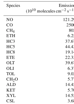
Table 2.VOC emissions in the FLUX test case.
Species Emission
(1010molecules cm−2s−1)
NO 121.29
CO 2500
CH4 802
ETH 6.25
HC3 37.67
HC5 44.43
HC8 19.14
ETE 22.33
OLT 39.67
OLI 6.37
TOL 9.02
CH2O 5.77
ALD 14.45
KET 5.70
XYL 14.55
CSL 3.68
Table 3.Initial conditions for the FLUX and STRATO test cases.
Species STRATO FLUX
vmr vmr
O3 1.0×10⁻⁶ 50×10−9
CO2 330×10−6 330×10−6
N2O 300×10−9 310×10−9
NO 1.0×10⁻⁹ 2.0×10⁻⁹
NO2 0.3×10⁻⁶ 1.0×10⁻⁹
HNO3 4.0×10⁻⁹ 0.5×10⁻⁹
CH4 1.4×10⁻⁶ 1.6×10⁻⁶
CO 20×10−9 150×10−9
HCl 2.5×10⁻⁹ 1.0×10⁻¹²
ClONO2 0.3×10⁻⁹ –
BrO 15×10−12 1.0×10⁻¹³
3.1 The FLUX case
The same FLUX case is integrated using the ASIS solver. In a first simulation noted A1, ASIS uses a RTOL value of 0.001 and a minimum time step of 1 s. For the solution of the linear system associated with ASIS, the DGESV code of the Lapack library is used. To compare with the Rosenbrock’s solver a second simulation A2 has been obtained with the same settings as A1 but with a higher relative tolerance value of 0.01, and a third one A3 with a tolerance value of 0.025. For all experiments the FLUX case is integrated over 24 h. The settings used in the overall simulations are given in Ta-ble 4.
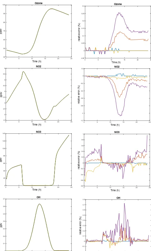
Figures 1 and 2 show the evolution of some key species for each experiment and the relative differences from the R1 experiment. Those results are representative of all of the species. As expected, the R1, G1, and A1 simulations give very close results. R1 and G1 show relative differences below 0.1 %, consistent with the value chosen for RTOL. A1 results are comparable with differences in the 0.1–0.2 % range, ex-cept at the beginning of the simulation when the chemical state is out of equilibrium and during day–night transitions. In those situations the differences between A1 and R1 or G1 can reach 0.5 %. As expected from the choice of a higher value for RTOL, the A2 experiment shows less accuracy but is still in the range of 0.5 % compared to the other experi-ments. The A3 experiment has differences below 2 % with the other experiments. For most of the atmospheric simula-tions an accuracy below 1 % is sufficient for the longest-lived species, and even larger values are acceptable for short-lived species if they are transient, given the uncertainties in the representation of the other processes and the inaccuracies in-troduced by their solution by a series of successive operators. The efficiency of ASIS can be first evaluated by compar-ison of the mean time steps (Table 4). For simulations R1 and G1 the mean time steps are between 25 and 40 s. Since ASIS uses a first-order scheme to maintain good accuracy, the mean time step is lowered, in the 5 s range for the A1 experiment. However, ASIS is a one-stage scheme (only one linear system is solved by time step) compared to R1 and G1 that need three or more stages. The amount of computation is therefore comparable. When the relative tolerance is in-creased, the mean time step of ASIS increases. For the A2 experiment it is 25 s, identical to R1, and up to 49 s for A3. Since for most atmospheric simulations a relative tolerance of 0.01 to 0.025 seems to be sufficient, the ASIS solver gives acceptable solutions with less computation than the higher-order schemes.
The efficiency of ASIS in terms of CPU time has been evaluated within the Matlab environment. Table 4 gives the ratio of CPU time used for each simulation relative to the R1 case. The ode23s code used to run the R cases needs the implementation of two subroutines, one that computes the species tendencies and one that gives the Jacobian of the sys-tem. If the latter is not provided, the ode23s code computes an approximation of the Jacobian by differentiation and the CPU cost increases by a factor of 2 to 10. As can be seen from
Table 4, the CPU cost of ASIS is comparable to or lower than the ode23s cost for relative tolerance values larger than 0.01. An important point to mention is that within the Matlab environment the CPU cost does not come from the linear al-gebra parts of the algorithms but from the evaluation of ten-dencies and Jacobian matrices. Therefore it is very dependent upon the chemical system and the details of the programming of the associated subroutines. The situation is quite different within the Fortran environment. With the Fortran version of ASIS the CPU cost for the calculation of the approximated Jacobian (the matrixMof Eq. 7) is negligible compared to the linear algebra computations. This is because the compiler efficiently handles the associated subroutine (fill_matrix, see Sect. 7) that contains frequent indirect addressing. It is not possible to evaluate if this is also the case with all the codes based on Rosenbrock’s algorithm, but if it is so, ASIS should perform well when the mean time steps are comparable since it needs fewer linear algebra computations.
For the A experiments, ASIS uses the DGESV code for the solution of the linear systems. To save computational time two iterative solvers have been tested, one using the Gauss– Seidel algorithm, the other the GMRES method. Both solvers used the same criterion for convergence (tolerance for con-vergence set to 10−14). For the GMRES method the precon-ditioning technique described in Sect. 2.1 is implemented. With those settings the experiment A2 has been repeated.
The results are practically identical to the solution ob-tained using the DGESV code; the differences between the solutions are below 0.02 % for all the species concentrations. The simulation with the Gauss–Seidel algorithm shows good efficiency in terms of mean number of iterations, but requires 6 to 10 times more iterations when the system is driven out of equilibrium during day–night transitions. Using GMRES was found to be more stable and efficient, with less than 10 it-erations needed to solve the linear systems and half as much computational time (using the Fortran version of the code) compared to the simulation using DGESV.
From the simulations of this FLUX case, which is rather representative of situations encountered in polluted earth boundary layers, it can be concluded that the ASIS solver performs well compared to higher-order schemes when mod-erate accuracy is required. Apart from tolerance parameters and the choice of a minimum time step, no specific tuning is required. The one-step implicit scheme gains in efficiency when coupled to the GMRES iterative solver used for the so-lution of the linear systems.
3.2 The STRATO case
The STRATO case differs from the FLUX case in the domi-nant chemical regimes involved. In the FLUX case the VOC decomposition during day and night dominates the system. With the STRATO case the chemistry is dominated by NOx,
HOx, Clxcatalytic cycles, and the ozone content. The
Table 4.List of the different settings used by the 0-D model for the FLUX test case. The mean time step is denoted byδtmand CPU-Ratio
is the CPU time used in each simulation relative to R1. The simulations are performed in the MATLAB environment.
R1 R2 R3 G1 A1 A2 A3
Method/code Rosen./ode23s Rosen./ode23s Rosen./ode23s Gear/ode15s ASIS ASIS ASIS
RTOL 0.001 0.01 0.025 0.001 0.001 0.01 0.025
δtm 39 s 44 s 46 s 25 s 4.7 s 25 s 49 s
CPU-Ratio 1 0.94 0.92 0.82 3.8 0.97 0.72
0 5 10 15 20 25
T ime (h) 40 50 60 70 80 90 100 ppbv Ozone
0 5 10 15 20 25
T ime (h) -0.05 0 0.05 0.1 0.15 0.2 0.25 0.3
relative error (%)
Ozone
0 5 10 15 20 25
T ime (h) 1.5 2 2.5 3 3.5 4 4.5 5 5.5 6 ppbv NO2
0 5 10 15 20 25
T ime (h) -1.2 -1 -0.8 -0.6 -0.4 -0.2 0 0.2
relative error (%)
NO2
0 5 10 15 20 25
T ime (h) 0 20 40 60 80 100 120 140 pptv NO3
0 5 10 15 20 25
T ime (h) -0.8 -0.6 -0.4 -0.2 0 0.2 0.4 0.6 0.8 1
relative error (%)
NO3
0 5 10 15 20 25
T ime (h) 0 0.1 0.2 0.3 0.4 0.5 0.6 0.7 pptv OH
0 5 10 15 20 25
T ime (h) -0.2 -0.1 0 0.1 0.2 0.3 0.4 0.5 0.6 0.7 0.8
relative error (%)
OH
Figure 1. FLUX case. Time evolution of selected species (O3,NO2,NO3,OH) for the R1, G1, A1, A2, and A3 experiments.
The left column shows the volume mixing ratios and the right one the differences in percentage (%) relative to the R1 experiment. The color code is the following: blue for G1, orange for A1, red for A2, and purple for A3.
0 5 10 15 20 25
T ime (h) 0 1 2 3 4 5 6 7 8 9 C o n c e n tr a ti o n ( m o le c c m ) 3
×1010 CH2O
0 5 10 15 20 25
T ime (h) 0 0.5 1 1.5 2 2.5 C o n c e n tr a ti o n ( m o le c c m ) 3
×107 HC8P
0 5 10 15 20 25
T ime (h) 0 0.5 1 1.5 2 2.5 3 ppbv
×1010 PAN
0 5 10 15 20 25
T ime (h) -0.5 -0.4 -0.3 -0.2 -0.1 0 0.1 0.2 0.3 0.4 0.5 R e la ti v e e rr o r (% ) CH2O
0 5 10 15 20 25
T ime (h) -2 -1.5 -1 -0.5 0 0.5 1 1.5 2 R e la ti v e e rr o r (% ) HC8P
0 5 10 15 20 25
T ime (h) -0.7 -0.6 -0.5 -0.4 -0.3 -0.2 -0.1 0 0.1 0.2 0.3 R e la ti v e e rr o r (% ) PAN
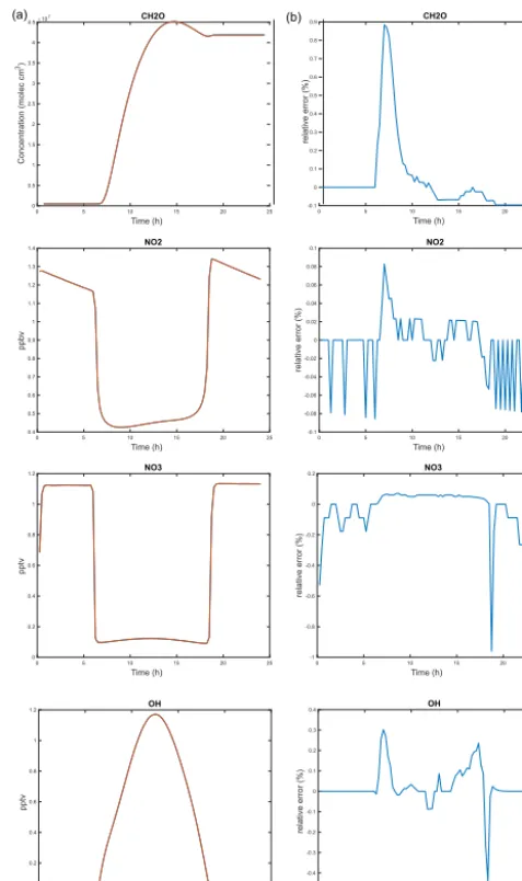
Figure 2.FLUX case. Same as Fig. 1 for CH2O, HC8P (peroxy
radicals), and PAN (peroxyacetyl nitrate).
concentrations of the species are tightly linked to the varia-tions of the insulation at sunrise and sunset.
simu-0 5 10 15 20 25
T ime (h)
0 50 100 150 200 250 300
N u
m b e r o f t im e s te p s
RTOL = 0.01, dtmin = 1 s
Figure 3.STRATO case. Number of time steps of the ASIS solver for each interval of 15 min in experiment AS2.
lation that starts in a situation out of equilibrium, the largest values are found at sunrise and sunset in the 150–200 range. It corresponds to time steps of about 4.5 s.
In terms of accuracy, the AS2 experiment gives results that depart less than 1 % compared to RS1. This is consistent with the chosen value of 0.01 for RTOL. Figure 4 shows that the lowest accuracy is found at sunrise and sunset when the short-lived radical species have the largest variations. Those transition situations are the most difficult because not only must the accuracy be maintained but spurious numerical os-cillations must be avoided. ASIS performs well here and adapts its time step automatically to reach the required ac-curacy. The numerical treatment adopted to calculate an ap-proximation of the Jacobian (Eq. 9 with β=1) contributes greatly to the reduction of numerical oscillations without sig-nificant degradation of the accuracy of the solution.
Equally, the approximations in the Jacobian are efficient to prevent the development of negative mixing ratios. In the two cases FLUX and STRATO, we did not encounter any signifi-cant (larger than ATOL) negative values during the course of the simulation, and all the concentrations remain positive at the end of the 15 min intervals before the photodissociation rates are updated.
In summary, the results of the two test cases confirm the properties targeted in the design of ASIS. At the moder-ate accuracy required for atmospheric simulations, the ASIS solver compares well with higher-order schemes, and lim-its the computational cost while assuring mass conservation. The next sections illustrate how it performs in more realis-tic situations with implementations in state-of-the-art global CTMs for Earth and Mars atmospheres.
0 5 10 15 20 25
T ime (h) 0 0.5 1 1.5 2 2.5 3 3.5 4 4.5 C o n c e n tr a ti o n ( m o le c c m ) 3
×107 CH2O
0 5 10 15 20 25
T ime (h) 0.4 0.5 0.6 0.7 0.8 0.9 1 1.1 1.2 1.3 1.4 ppbv NO2
0 5 10 15 20 25
T ime (h) 0 0.2 0.4 0.6 0.8 1 1.2 pptv NO3
0 5 10 15 20 25
T ime (h) 0 0.2 0.4 0.6 0.8 1 1.2 pptv OH
0 5 10 15 20 25
T ime (h) -0.1 0 0.1 0.2 0.3 0.4 0.5 0.6 0.7 0.8 0.9
relative error (%)
CH2O
0 5 10 15 20 25
T ime (h) -0.1 -0.08 -0.06 -0.04 -0.02 0 0.02 0.04 0.06 0.08 0.1
relative error (%)
NO2
0 5 10 15 20 25
T ime (h) -1 -0.8 -0.6 -0.4 -0.2 0 0.2
relative error (%)
NO3
0 5 10 15 20 25
T ime (h) -0.5 -0.4 -0.3 -0.2 -0.1 0 0.1 0.2 0.3 0.4
relative error (%)
OH
(a) (b)
Figure 4. STRATO case. Time evolution of selected species (CH2O,NO2,NO3,OH) for the RS1, and AS2 experiments. (a)shows the mixing ratios or concentrations and(b)the differences in percentage (%) for AS2 relative to the RS1 experiment.
4 Implementation within the MOCAGE model
October 2011. Wind and temperature fields come from the operational weather analyses of the ECMWF. They are up-dated every 3 h and linearly interpolated in between these time intervals.
The reference simulation (referred to hereafter as MR) uses the original solver for chemistry, an iterative semi-implicit scheme with assumptions of equilibrium for short-lived species and species lumping for NOxand Clxfamilies.
The chemical time step varies with altitude but is kept con-stant during the model integration. It increases from 20 s in the planetary boundary layer to 15 min in the stratosphere.
The simulation with the ASIS solver, MA, uses the same configuration for MOCAGE as MR except that the original chemical solver is replaced by ASIS with set-tings similar to experiment A3: RTOL=0.025, ATOL= 104molecules cm−3, a minimum time step of 5 s, and the GMRES solver for the solution of the linear systems.
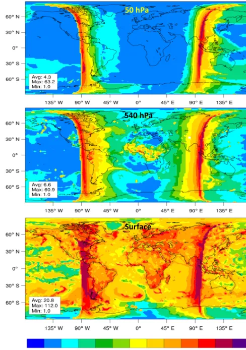
The characteristics of the ASIS functioning implemented within MOCAGE can be first examined by the diagnostic of the number of sub-time-steps for chemistry. Figure 5 shows this number for three different levels for a date corresponding to 15 September at midday. In the midstratosphere, at 50 hPa, the number of sub-time-steps varies in accordance with what was found for the STRATO test case. At midday or midnight the chemical system is in quasi-steady-state and this num-ber is small, below 3. Close to the terminators, this numnum-ber increases up to 40–60, highlighting the change of regime of the chemical system when the photodissociation is activated or deactivated. During these transition phases the stiffness of the system increases and the sub-time-steps decrease to maintain the required accuracy. Also barely noticeable is an increase of the number of sub-time-steps over the Antarctic coast at the edge of the polar vortex. In these regions the het-erogeneous reactions acting at the surface of polar clouds are activated, driving the concentrations of the chlorine species out of equilibrium. It leads to a reduction of the sub-time-steps to cope with the rapid variations of the chemical com-position of the air masses.
In the middle troposphere the same behavior is encoun-tered near the terminators, with a tendency to maintain re-duced sub-time-steps during longer periods after sunrise or before sunset (Fig. 5). An increase of the number of sub-time-steps is also encountered over the African continent at low latitudes. Those regions are prone to convective activity, and injection of species by convection is activated, leaving air masses far from chemical steady state. Since the chemi-cal evolution of the species is chemi-calculated after the transport processes, ASIS starts with a situation far from a chemical equilibrium and the number of sub-time-steps increases.
At the surface, Fig. 5 shows the same characteristics as in the midtroposphere with an increase of the number of sub-time-steps at the terminators and over the continents. Over the continents the surface emissions play a larger role than convection in destabilizing the chemical system. Within MOCAGE the emissions are calculated according to
inven-Figure 5.Number of sub-time-steps per time step of 15 min in the MA simulation for the 15 September at midday. Three levels are presented representative of the stratosphere (50 hPa), the midtropo-sphere (540 hPa), and the surface.
tories and deposited in the boundary layer. This is treated as an isolated process that changes the concentrations. As a re-sult ASIS starts with situations out of chemical equilibrium and adopts small sub-time-steps, about 20 s compared to 60 s over the oceans.
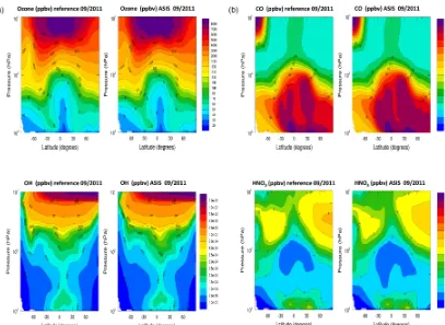
Except for noticeable cases that are discussed hereafter, the species distributions of the simulation with the ASIS solver (referred to hereafter as MA) are close to those ob-tained in MR. As an illustration, Fig. 6 shows the zonally av-eraged distributions of O3,CO,OH, and HNO3for the month
of September. In most altitudes the differences are below 10 %, with the largest differences in Southern Hemisphere high latitudes in the lower stratosphere. Similar differences are found for the other species, except for the NOx species
in the lower troposphere and the chlorine species in the high latitudes of the Southern Hemisphere during the formation of the stratospheric ozone hole.
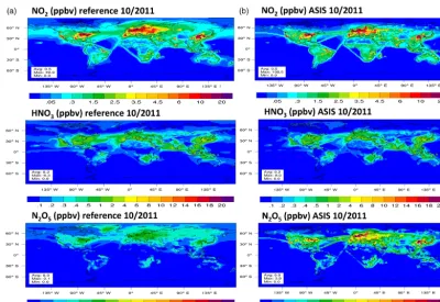
assumptions are made for the computation of the nighttime NO2/NO3/N2O5system. These approximations are valid in
the stratosphere but fail in the lower troposphere where the pressure and temperature are larger. As a result the MR sim-ulation underevaluates the concentrations of NO3and N2O5.
Figure 7 shows, for example, the distributions of NO2,HNO3, and N2O5 at the lower level near the surface
averaged over the month of October. In the region of sur-face emissions, the MR simulation strongly underestimates the N2O5concentrations. Since the chemical scheme adopted
for the present simulations does not include the formation of HNO3by the hydrolysis reaction of N2O5on aerosol surface
(Dentener and Crutzen, 1993), it does not have a major influ-ence on the other species. Nevertheless, the maximum values for HNO3and NO2are larger in the MA simulation than in
the MR simulation.
Another significant difference between MR and MA is found in the simulation of the ClOx system in the lower
stratosphere at high Southern Hemisphere latitudes. In late August and early September, the solar radiation comes back at high latitudes and the lower stratospheric O3is destroyed
by catalytic cycles involving chlorine radicals (Solomon, 1999). The chlorine radical concentrations are enhanced by the heterogeneous reactions on polar stratospheric clouds’ (PSCs) surface that convert HCl and ClONO2into Cl2that
is photodissociated to form the chlorine radicals. In addi-tion, the catalytic destruction of O3also involves the bromine
species.
In the air masses prone to heterogeneous reactions on PSC, the composition changes rapidly at sunrise and non-linear processes, like the formation of Cl2O2, a key species for the
O3 destruction, play a major role. As a result the chemical
system is very stiff and the ASIS solver diminishes the chem-ical time step to a few seconds to maintain good accuracy. In these transient situations the original code in MR does not change its settings and a fixed time step of 15 min is used.
As a result, the MR simulation produces a much more pronounced ozone depletion over Antarctica than the MA simulation. MR calculates ozone column contents as low as 100 Dobson Units (DU), whereas the MA simulation maintains values in the range of 150 DU. This is well illus-trated in Fig. 8, which shows the evolution of the total ozone columns over two Antarctic stations, Dumont d’Urville and Dome C. For these two stations the measurements done by SAOZ instruments (Pommereau and Goutail, 1988) at sun-rise and sunset are also presented (data available at http: //saoz.obs.uvsq.fr/).
Starting around Julian day 220, the MR and MA simu-lations start to diverge. Over Dumont d’Urville, the station that sees first the return of the sunlight, the ozone decrease is about 50 % larger in the MR simulation than for MA. By day 260 the ozone column is just above 150 DU whereas it is in the 200 DU range in the MA simulation. Clearly the MA simulation is in better agreement with the SAOZ measure-ments.
The same behavior is seen for the Dôme C station. The ozone depletion starts slightly later, around day 240. In the MR simulation the depletion is very pronounced and the ozone column diminishes rapidly in a few days from 240 to 150 DU, and further decreases at a slower rate to reach a minimum of 100 DU at day 260. The MA simulation shows a more continuous decrease from day 240 to 260, with an ozone column reaching a minimum of 150 DU. The MA sim-ulation is here again in very good agreement with the SAOZ observations.
Implementation of the ASIS solver within MOCAGE has thus revealed two weaknesses of the original model. One problem is in a limitation on the validity of assumptions made to compute the night-time distribution of the NOx
species. It can be solved by adequate coding. The other one is a lack of accuracy in the solution of the chemical system in specific situations in the lower stratosphere. This can cer-tainly be avoided by a drastic reduction of the time step, but it would need the implementation of a time-varying time step strategy somewhat similar to the one adopted for ASIS.
Clearly the implementation of ASIS within MOCAGE is very beneficial to the model simulations and increases the confidence on the model results. In addition, further evo-lution of the model with adoption of different chemical schemes or addition of new reactions is very easy with ASIS. There is, however, a price to pay in terms of computer time. Overall the MA simulation takes 4.7 times more com-putational time than the MR simulation. This number could certainly be decreased by further tuning of the parameters of the solver, RTOL, ATOL, andδtmin, and maybe also by
the use of the Gauss–Seidel algorithm instead of GMRES in situations where the solution of the linear system converges easily.
Our experience with ASIS shows that, since various pro-cesses are computed by a series of operators, the solver starts new time steps with situations often out of chemical equilib-rium and must use small sub-time-steps. To alleviate this, one possibility is that tendencies from these operators would be computed and stored rather than used to update the species concentrations. The tendencies can then be used to solve the system though their introduction in the term F of Eq. (7). We have tested this option for the species emissions at the surface and found that the number of sub-time-steps is de-creased by a factor of 2 in the lower troposphere. It remains to be seen if other processes can be treated that way. Emis-sions are the most straightforward because the resulting ten-dencies are positive and cannot lead to the calculation of neg-ative concentrations.
Figure 6.Zonal mean distributions of O3,CO,OH, and HNO3for the month of September. The panels in(a)show results for the reference
simulation, MR; those in(b)show results of the MA simulation with the use of the ASIS solver.
the stratosphere and upper troposphere more computer time is needed near the terminators and in case of PSC-induced chemistry. In the lower troposphere more computer time is spent in grid points influenced by surface emissions, and con-vective and boundary-layer transport processes. A speedup of 15 was, however, obtained for the MA simulation on our cluster computer (using 1 node and 16 cores of our BULL computer) with a decomposition that groups more longi-tudes in the Southern Hemisphere than in the Northern Hemi-sphere, near the poles. But further tuning would be required if more nodes are to be used. This tuning could vary with sea-son and additional parallelization could be introduced with domain decomposition on the vertical.
5 Implementation within the LMD Mars model
To illustrate the versatility of the ASIS solver, we present re-sults of the implementation of ASIS in the LMD Mars model with photochemistry (Lefèvre et al., 2004). This Mars GCM describes the evolution of 19 species (Table 5) by means of 54 chemical or photolytic reactions. The bulk atmosphere of Mars is composed of 95 % CO2with trace amounts of H2O.
As a result, the only processes that initiate Martian photo-chemistry are the photolysis of CO2and H2O by ultraviolet
solar light. Therefore, the photochemistry of the lower
at-Table 5.List of species used in the Mars model simulations.
O(1D),O(3P),O2,O3,
N,N2,NO,NO2,N(2D),
H2,H2O(gas & solid),H,OH,HO2,H2O2,
CO,CO2,Ar
mosphere of Mars can be summarized by the interactions be-tween the oxygenated species O(1D), O, and O3produced by
CO2photolysis and the hydrogen radicals H, OH, and HO2
produced by H2O photolysis. These processes are similar to
those occurring in the Earth’s mesosphere, with comparable conditions of pressure and temperature.
photo-Figure 7.Monthly mean distributions of NO2,HNO3, and N2O5at the surface for the month of October after a 2 month integration. The
panels in(a)show results of the reference simulation, MR; those in(b)show results of the MA simulation with the use of the ASIS solver. The MR simulation underevaluates the N2O5in the lower troposphere.
210 220 230 240 250 260 270 280 290 300 310
J ulian days
150 200 250 300 350 400 450
Dobson units
Ozone column over Dumont d' Urville, 2011
210 220 230 240 250 260 270 280 290 300 310
J ulian days
100 150 200 250 300 350
Dobson units
Ozone column over Dome C, 2011
Figure 8.Evolution of the total ozone column over the Dumont d’Urville and Dome C Antarctic stations. The dots are the observations of the SAOZ instrument, the orange line is the evolution calculated in the reference simulation, MR, and the red line the same output from the simulation MA using the ASIS solver.
chemical equilibrium are used to increase accuracy and avoid very small time steps. However, conditions of photochemical equilibrium change at night and are also very dependent on altitude. For instance, on Mars, the lifetimes of O(3P)and H vary between less than 1 s near the surface and several years at 100 km. Such stark variation prevents the assump-tion of photochemical equilibrium or use of Eq. (3) through-out the atmosphere. Thus, despite its apparent simplicity, the EB method may complicate the problem by requiring
dif-ferent treatments for specific species or specific parts of the atmosphere.
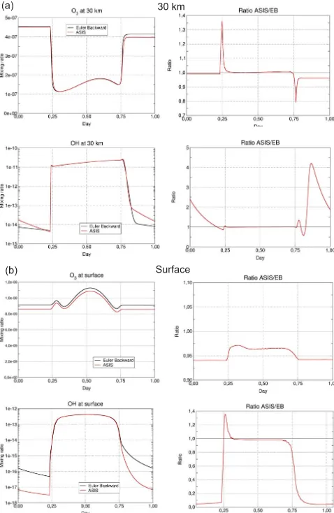
Figure 9. Comparison of the Euler-backward (EB) and ASIS solvers applied to the Mars box-model version. The left column shows the mixing ratios of O3 and OH and the right one the
ra-tio between the ASIS and EB experiments. Results are presented at 30 km(a)and at the surface(b), for equatorial conditions in north-ern spring (solar longitude Ls=70◦). Local noon is at day 0.5.
model adapted to Mars. The time step of the EB solver is fixed toδt=7.5 min as done in the Mars GCM. ASIS uses the variable stepsize strategy described in Sect. 2.3, bounded by a maximum value of 15 min and the minimum time step of 10 s. RTOL is fixed to 0.05 and the ATOL density corre-sponds to a volume mixing ratio of 10 ppt. ATOL is therefore variable with altitude. The solution of the linear systems as-sociated with ASIS is done using the DGESV direct solver. We found that these settings were adequate to reach a satis-fying compromise between accuracy and computing time.
At the surface, Fig. 9 shows that the ASIS solver calculates an O3mixing ratio that is lower by 3 to 6 % compared to the
EB solver. This difference is related to the lack of accuracy in the treatment of the HOxspecies in the EB solver, which
assumes that OH and HO2are at photochemical equilibrium
at all times within the HOx family. This assumption is close
to reality during the day, but becomes problematic at sunrise and sunset and is wrong at night, when the HO2lifetime can
reach several hours at the surface. As a result, the OH mixing ratio calculated by the EB solver is overestimated by a factor of 10 compared to ASIS, which does not require any a pri-ori assumption on chemical lifetimes and provides an accu-rate solution throughout sunset and nighttime. At sunrise and sunset ASIS reduces the chemical time step down to 10 s to solve the sharp transitions in the concentrations of short-lived species H, OH, O, and NO. Outside these critical (but short) periods, the Martian settings of RTOL and ATOL allow time steps that increase rapidly and may reachδt=15 mn without sacrificing the accuracy. Thus, in the example of Fig. 9, at the surface level, the number of chemical time steps performed by ASIS over 1 Martian day is only 12 % larger than in the EB simulation.
The box-model simulations at 30 km are performed at the hygropause level where the production rate of HOx radicals
by H2O photolysis is the largest. This results in a maximum
stiffness of the system at sunrise and sunset, when the H2O
photolysis rate varies rapidly. Those critical day–night tran-sitions show large differences between the ASIS and the EB simulations. In the EB run, ozone is integrated implicitly by Eq. (3) at night and is assumed to be at photochemical equilibrium within the Oxfamily during the day. This abrupt
change in treatment contrasts with the smooth transition car-ried out with the time-step-adaptive scheme of ASIS. At the price of a strong reduction of the time step to maintain the required accuracy, ASIS calculates an O3 mixing ratio that
is respectively 35 % larger and 20 % smaller than in the EB run at sunrise and sunset. Both solvers give the same results during the day. However, the more accurate description of the O3increase at sunset by ASIS induces a 5 % difference
with the EB solver that persists into the night. Regarding OH, the simulation at 30 km confirms the weakness of the steady-state approximation for HOx at night in the EB scheme. In
ASIS, the stiffness of the system diagnosed by the solver re-mains high in the first hours following sunset (due to strong curvature of the solution for H, not shown here) and leads to a reduction of the time step to about 30 s. The nighttime OH mixing ratio is larger by a factor of 2 to 4 than in the EB simulation. For this extreme case of stiffness in the Mars at-mospheric chemistry, the total number of chemical time steps executed by ASIS over one Martian day is 65 % larger than in the EB simulation.
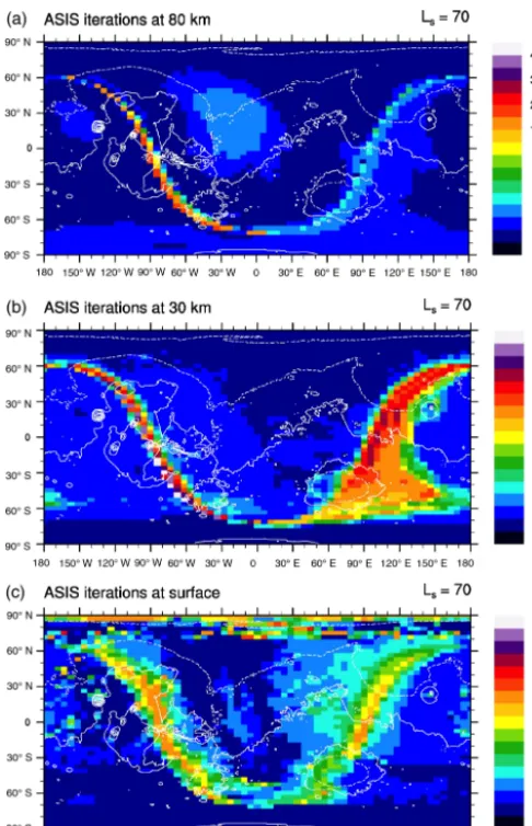
In its 3-D implementation, ASIS is called by the LMD GCM at each physical time step1t=15 mn. The ASIS set-tings in the GCM are identical to those of the box model pre-sented earlier, i.e., the solver may select any sub-time-step value between1t and the minimum valueδtmin=10 s. To
Figure 10. Number of sub-time-steps per time interval of 15 min in the LMD Mars GCM in northern spring (instantaneous result at solar longitude Ls=70◦and day 150 of the simulation). Three al-titude levels are represented at 80 km(a), 30 km(b), and the sur-face(c). Local noon is located at longitude zero. The white contour represents topography, with a 4 km interval.
Figure 10 shows the number of sub-time-steps per phys-ical time step of 15 mn in a GCM simulation of northern spring (Ls=70◦) using ASIS. For the three levels presented here (surface, 30 km, 80 km), the number of sub-time-steps is equal to 1 or 2 for a large fraction of time. This is the case when the chemical system is in equilibrium, far from the terminators at night or during the day. As in the MOCAGE model, at the terminators the number of sub-time-steps in-creases dramatically to cope with the change of chemical regime at the day–night transitions. The maximum number (40–50) is found at sunrise at 30 km and is essentially driven by the abrupt changes in OH and O3already seen in Fig. 10.
At the surface, an increase in the number of sub-time-steps is also visible near the North Pole. This is related to fast het-erogeneous reactions of HOx species on water–ice clouds
(Lefèvre et al., 2008), a process similar to that occurring with chlorine on Earth stratospheric clouds. In those cases ASIS adopts a smaller time step to resolve with good accuracy a system that is locally away from chemical equilibrium.
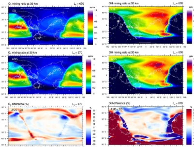
Figure 11 compares at 30 km the results of GCM simula-tions using either the EB or the ASIS solver. Both schemes give distributions of O3and OH that are in general very close
during daytime and away from the terminators. At the ter-minators, ASIS calculates O3amounts that are about 50 %
larger than EB at sunrise and 25 % smaller at sunset. These large differences are similar to those found with the box-model runs (Fig. 9) but are limited in time and space. How-ever, the better description of O3by ASIS across the
termi-nators may be crucial when comparing the GCM to Martian ozone measurements performed at the terminators by the so-lar occultation technique. Regarding OH, the GCM results confirm the poor description of the HOx chemistry by the
EB scheme at the terminators. At night, OH values calcu-lated by EB are more than 30 % smaller than with ASIS. The amount of nighttime OH is small relative to daytime values. Thus, the bias in the EB scheme does not significantly affect the oxidizing capacity of Mars simulated by the GCM. Nev-ertheless, similarly to ozone, the more accurate description of OH and the Martian nighttime chemistry in general is an important advantage brought by ASIS for the interpretation of the numerous observations of nightglow or measurements by stellar occultation carried out on that planet.
6 Conclusions
The ASIS solver has been designed to cope with the various situations encountered within the numerical simulation of the atmospheric chemistry. The main properties of the solver are mass conservation, an approximation of the Jacobian matrix of the chemical fluxes that stabilizes the associated system of differential equations, a time-stepping varying module to control accuracy, and a code implementation that allows an easy adaptation to various chemical schemes. In box-model test cases, the numerical solutions obtained with the ASIS solver were found to be in good agreement with those of mul-tistep algorithms like Rosenbrock’s and Gear’s methods.
The ASIS solver has been implemented in 3-D models of the Earth (MOCAGE) and Mars (LMD model) planets. The results with MOCAGE using ASIS reveals two weaknesses of the original semi-implicit solver. One is related to the cal-culation of the partitioning of the NOxspecies at the surface
and the other to an overestimation of the ozone depletion in the Antarctic stratospheric vortex in Spring. In the simulation of the Mars atmosphere ASIS gives more accurate simula-tions during day–night transisimula-tions and at night for the HOx
Figure 11.Distribution of O3(left) and OH (right) at 30 km calculated by the LMD Mars GCM in northern spring (instantaneous result at
solar longitude Ls=70◦and day 150 of the simulation). Top: Euler-backward (EB) solver. Middle: ASIS solver. Bottom: relative difference (%) between ASIS and EB, using thresholds of 10 ppbv for O3and 10 pptv for OH. Local noon is located at longitude zero. The white
contour represents topography, with a 4 km interval. Off-scale differences in O3and OH are limited to±50 % and±30 % respectively.
attributed to missing chemistry or misrepresentation of some physical processes.
The model simulations show the benefit of using a chem-ical solver with good properties such as mass conservation and controlled accuracy. This objective can be achieved us-ing multistep high-order algorithms, but the computational cost of those schemes increases rapidly with the number of species considered. Since ASIS is implicit and one-step, a single linear system has to be solved for each iteration. For this, direct or iterative algorithms can be used. The di-rect methods based on LU decomposition see their compu-tational cost increasing at least quadratically with the num-ber of species, whereas the cost of iterative solvers increases rather linearly. Within ASIS we found that the GMRES iter-ative algorithm is stable and efficient, and is competitive in terms of CPU cost compared to the direct DGESV algorithm. In atmospheric models the computational cost is a key issue, and parallelization of the computations must be effi-cient to reduce the elapsed time spent for the simulations. As pointed out earlier, the amount of computation spent by ASIS to solve the chemical system can vary significantly from one grid point to another. This renders the work balanc-ing of tasks more difficult if a domain decomposition strategy
is adopted to implement the parallelization. As already dis-cussed with the surface emissions, one possibility to dimin-ish the number of iterations and the heterogeneity in the CPU used at each grid point is to account for nonchemical tenden-cies in the spetenden-cies continuity equations (termF of Eq. 4). Rather than updating the concentrations after each process, the resulting tendencies could be added and integrated within ASIS. This strategy has been adopted by, for example, Menut et al. (2013) for the CHIMERE model; it remains to be seen if the stability and the positivity of the solution can be main-tained.
diminish and may result in reduced time steps and increased computer time.
In conclusion, the ASIS solver can deal with many situ-ations encountered in modeling atmospheric chemistry for a computational cost affordable by CTMs and GCMs that include comprehensive chemical schemes. Evolution of the ASIS solver to treat aqueous-phase chemistry is planned in the near future.
Code availability. The Fortran code to run the ASIS solver on the FLUX case described is Sect. 3 is available as a Supplement to the present article and can be downloaded from the CERFACS server (www.cerfacs.fr).
The code associated with the chemistry model includes subrou-tines that define the mechanism and those more specific to the ASIS solver. At this stage we have not developed an external driver or a pre-processor that would generate specific codes based on the adopted mechanism. This choice was done because our experience is that the maintenance of the driver outputs can be somewhat cum-bersome when many developers work in parallel on a CTM. In ad-dition, the code generated by the driver must be optimized often for the computer used and adapted to the CTM. It is therefore not used directly, which introduces further constraints on the maintenance of the overall code.
Our approach is rather to define the mechanism by a limited num-ber of fortran subroutines that are simply added to the other rou-tines of the code. Thenum_speciesroutine names and numbers the species, the indices_reactionsroutine does the same for the reac-tions. The reactions are classified in three groups:
1/ A→b B + c C 2/ A + A→b B + c C 3/ a A + b B→c C + d D
The first group includes photodissociations and thermal decom-position of the species. This classification is done in order to opti-mize the calculation of the terms of the matrixMof Eq. (7). Some reactions give more than 2 products and fractional sub-reactions must be introduced. For example, the following reaction with frac-tional products:
HC5P + NO3 → 0.021*HCHO + 0.239*ALD + 0.828*KET + 0.699*HO2 + 0.040*MO2 + 0.262*ETHP + 0.391*XO2 + NO2 will be decomposed in 4
sub-reactions within the indices_reactions routine:
zloc2=Z4SPEC(1.0,JPHC5P,1.0,JPNO3,0.021,JPHCHO,0.239, JPALD)
Zindice_4(JP4_HC5P_NO3_i)=zloc2
zloc2=Z4SPEC(0.0,JPHC5P,0.0,JPNO3,0.828,JPKET,0.699, JPHO2)
Zindice_4(JP4_HC5P_NO3_ii)=zloc2
zloc2=Z4SPEC(0.0,JPHC5P,0.0,JPNO3,0.040,JPMO2,0.262, JPETHP)
Zindice_4(JP4_HC5P_NO3_iii)=zloc2
zloc2=Z4SPEC(0.0,JPHC5P,0.0,JPNO3,0.391,JPXO2,1.0,JPNO2) Zindice_4(JP4_HC5P_NO3_iv)=zloc2, paying attention not to duplicate associated fluxes.
Once the definition of species and reactions is completed, the cal-culation of the matrices (Eq. 7) is done by thefill_matrixroutine, the time steps are monitored by thedefine_dtroutine, and the solution of the linear systems by theSolvesysroutine.
The Supplement related to this article is available online at doi:10.5194/gmd-10-1467-2017-supplement.
Competing interests. The authors declare that they have no conflict of interest.
Acknowledgements. This work was supported by the
Monitoring Atmospheric Composition and Climate
(http://www.gmes-atmosphere.eu/) and COPERNICUS
At-mospheric Monitoring Service (https://atmosphere.copernicus.eu/) EU projects. The authors thank Emanuele Emili, Andrea Piacen-tini, and Michael Prather for their very helpful comments on the manuscript.
Edited by: G. A. Folberth
Reviewed by: three anonymous referees
References
Ashino, R., Nagase, M., and Vaillancourt, R.: Behind and beyond the MATLAB ODE suite, Comput. Math., 40, 491–512, 2000. Audiffren, N., Renard, M., Buisson, E., and Chaumerliac, N.:
De-viations from the Henry’s law equilibrium during cloud events: a numerical approach of the mass transfer between phases and specific numerical effects, Atmos. Res., 49, 139–161, 1998. Bey, I., Jacob, D. J., Yantosca, R. M., Logan, J. A., Field, B., Fiore,
A. M., Li, Q., Liu, H., Mickley, L. J., and Schultz, M.: Global modeling of tropospheric chemistry with assimilated meteorol-ogy: Model description and evaluation, J. Geophys. Res., 106, 23073–23096, 2001.
Carver, G. D. and Stott, P. A.: IMPACT: an implicit time integration scheme for chemical species and families, Ann. Geophys., 18, 337–346, doi:10.1007/s00585-000-0337-y, 2000.
Crassier, V., Suh, K., Tulet, P., and Rosset, R.: Development of a reduced chemical scheme for use in mesoscale meteorological models, Atmos. Environ., 34, 2633–2644, 2000.
Dentener, F. J. and Crutzen, P. J.: Reaction of N2O5on tropospheric
aerosols: impact on the global distributions of NOx, O3, and OH,
J. Geophys. Res.-Atmos, 98, 7149–7163, 1993.
Emmons, L. K., Walters, S., Hess, P. G., Lamarque, J.-F., Pfister, G. G., Fillmore, D., Granier, C., Guenther, A., Kinnison, D., Laepple, T., Orlando, J., Tie, X., Tyndall, G., Wiedinmyer, C., Baughcum, S. L., and Kloster, S.: Description and evaluation of the Model for Ozone and Related chemical Tracers, version 4 (MOZART-4), Geosci. Model Dev., 3, 43–67, doi:10.5194/gmd-3-43-2010, 2010.
Golub, G. H. and Van Loan, C. F.: Matrix computations, Johns Hophins Univ. Press, 4th Edn., 2013.
González-Galindo, F., Forget, F., López-Valverde, M. A., Ange-lats i Coll, M., and Millour, E.: A ground-to-exosphere Martian general circulation model: 1. Seasonal, diurnal, and solar cycle variation of thermospheric temperatures, J. Geophys. Res., 114, E04001, doi:10.1029/2008JE003246, 2009.
Hesstvedt E., Hov, O., and Isaksen, I.: A quasi-steady state approx-imation in air pollution modelling: comparison of two numerical schemes for oxidant prediction, Int. J. Chem. Kinet., 10, 971– 994, 1978.
Hindmarsh, A. C.: ODEPACK: A systematized collection of ODE solvers, in: IMACS Trans. on Scientific Computation, Vol. 1, Sci-entific Computing, edited by: Stepleman, R. S., North-Holland, Amsterdam, 1980.
Huijnen, V., Williams, J., van Weele, M., van Noije, T., Krol, M., Dentener, F., Segers, A., Houweling, S., Peters, W., de Laat, J., Boersma, F., Bergamaschi, P., van Velthoven, P., Le Sager, P., Es-kes, H., Alkemade, F., Scheele, R., Nédélec, P., and Pätz, H.-W.: The global chemistry transport model TM5: description and eval-uation of the tropospheric chemistry version 3.0, Geosci. Model Dev., 3, 445–473, doi:10.5194/gmd-3-445-2010, 2010.
Jacobson, M. Z. and Turco, P.: SMVGEAR: A sparse-matrix, vec-torized GEAR code for atmospheric models, Atmos. Environ., 28, 273–284, 1994.
Josse, B., Simon, P., and Peuch, V.-H.: Rn-222 global simula-tions with the multiscale CTM MOCAGE, Tellus, 56B, 339–356, 2004.
Lefèvre, F., Brasseur, G. P., Folkins, I., Smith, A. K., and Simon, P.: Chemistry of the 1991/1992 stratospheric winter: Three di-mensional model simulations, J. Geophys. Res., 99, 8183–8195, 1994.
Lefèvre, F., Lebonnois, S., Montmessin, F., and Forget, F.: Three-dimensional modeling of ozone on Mars, J. Geophys. Res., 109, E07004, doi:10.1029/2004JE002268, 2004.
Lefèvre, F., Bertaux, J.-L., Forget, F., Lebonnois, S., Montmessin, F., Fast, K., Clancy, R. T., and Encrenaz, T.: Heterogeneous chemistry in the atmosphere of Mars, Nature, 414, 971–975, 2008.
Leriche, M., Pinty, J.-P., Mari, C., and Gazen, D.: A cloud chemistry module for the 3-D cloud-resolving mesoscale model Meso-NH with application to idealized cases, Geosci. Model Dev., 6, 1275– 1298, doi:10.5194/gmd-6-1275-2013, 2013.
Madronich, S. and Flocke, S.: The Role of Solar Radiation in Atmo-spheric Chemistry, Springer-Verlag, New York, 126 pp., 1998. Menut, L., Bessagnet, B., Khvorostyanov, D., Beekmann, M.,
Blond, N., Colette, A., Coll, I., Curci, G., Foret, G., Hodzic, A., Mailler, S., Meleux, F., Monge, J.-L., Pison, I., Siour, G., Turquety, S., Valari, M., Vautard, R., and Vivanco, M. G.: CHIMERE 2013: a model for regional atmospheric composition modelling, Geosci. Model Dev., 6, 981–1028, doi:10.5194/gmd-6-981-2013, 2013.
Michou, M. and Peuch, V.-H.: Surface exchanges in the multi-scale chemistry and transport model MOCAGE, Water Sci. Rev., 15, 173–203, 2002.
Mott, D. R., Oran, E. S., and van Leer, B.: A Quasi-Steady-State Solver for the Stiff Ordinary Differential Equations of Reaction Kinetics, J. Comp. Phys., 164, 407–428, 2000.
O’Connor, F. M., Johnson, C. E., Morgenstern, O., Abraham, N. L., Braesicke, P., Dalvi, M., Folberth, G. A., Sanderson, M. G., Telford, P. J., Voulgarakis, A., Young, P. J., Zeng, G., Collins, W. J., and Pyle, J. A.: Evaluation of the new UKCA climate-composition model – Part 2: The Troposphere, Geosci. Model Dev., 7, 41–91, doi:10.5194/gmd-7-41-2014, 2014.
Pommereau, J. P. and Goutail, F.: Stratospheric O3 and
NO2 Observations at the Southern Polar Circle in
Sum-mer and Fall 1988, Geophys. Res. Lett., 15, 895–897, doi:10.1029/GL015i008p00895, 1988.
Pozzoli, L., Bey, I., Rast, S., Schultz, M. G., Stier, P., and Feichter, J.: Trace gas and aerosol interactions in the fully coupled model of aerosol-chemistry-climate ECHAM5-HAMMOZ: 1. Model description and insights from the spring 2001 TRACE-P experiment, J. Geophys. Res., 113, D07308, doi:10.1029/2007JD009007, 2008.
Ramaroson, R. A., Pirre, M., and Cariolle, D.: A box model for on-line computations of diurnal variations in a 1-D model: potential for application in multidimensional cases, Ann. Geophys., 10, 416–428, 1992.
Rosenbrock, H. H.: Some general implicit processes for the numer-ical solution of differential equations, Comput. J., 5, 329–330, 1963.
Saad, Y.: Iterative Methods for Sparse Linear Systems, 2nd Edn., SIAM, Philadelphia, 2003.
Saad, Y. and Schultz, M. H.: GMRES: A generalized minimal resid-ual algorithm for solving nonsymmetric linear systems, SIAM J. Sci. Stat. Comput., 7, 856–869, doi:10.1137/0907058, 1986. Sandu, A. and Sander, R.: Technical note: Simulating chemical
systems in Fortran90 and Matlab with the Kinetic PreProcessor KPP-2.1, Atmos. Chem. Phys., 6, 187–195, doi:10.5194/acp-6-187-2006, 2006.
Sandu, A., Verwer, J. G., Van Loon, M., Carmichael, G. R., Potra, F. A., Dabdub, D., and Seinfeld, J. H.: Benchmarking stiff ode solvers for atmospheric chemistry problems I: Implicit vs Ex-plicit, Atmos. Environ., 31, 3151–3166, 1997a.
Sandu, A., Verwer, J. G., Blom, J. G., Spee, E. J., Carmichael, G. R., and Potra, F. A.: Benchmarking stiff ode solvers for atmospheric chemistry problems II: Rosenbrock solvers, Atmos. Environ., 31, 3459–3472, 1997b.
Shampine, L. F. and Reichelt, M. W.: The
MAT-LAB ODE Suite, SIAM J. Sci. Comput., 18, 1–22,
doi:10.1137/S1064827594276424, 1997.
Solomon, S.: Stratospheric ozone depletion: A review
of concepts and history, Rev. Geophys., 37, 275–316, doi:10.1029/1999RG900008, 1999.
Stockwell, W. R., Kirchner, F., Kuhn, M., and Seefeld, S.: A New Mechanism for Regional Atmospheric Chemistry Modeling, J. Geophys. Res., 102, 25847–25879, 1997.
Stott, P. A. and Harwood, R. S.: An implicit time-stepping scheme for chemical species in a global atmospheric circulation model, Ann. Geophys., 11, 377–3888, 1993.
Suhre, K. and Rosset, R.: Modification of a linearized semi-implicit scheme for chemical reactions using a steady-state-approximation, Ann. Geophys., 12, 359–361, 1994.