www.geosci-model-dev.net/9/4313/2016/ doi:10.5194/gmd-9-4313-2016
© Author(s) 2016. CC Attribution 3.0 License.
Parameter interactions and sensitivity analysis for modelling carbon
heat and water fluxes in a natural peatland, using CoupModel v5
Christine Metzger1,a, Mats B. Nilsson2, Matthias Peichl2, and Per-Erik Jansson1
1Department of Land and Water Resources Engineering, Royal Institute of Technology, Stockholm, 100 44, Sweden 2Department of Forest Ecology and Management, Swedish University of Agricultural Sciences, Umeå, 901 83, Sweden anow at: Institute for Meteorology and Climate Research/Atmospheric Environmental Research (IMK-IFU),
Karlsruhe Institute for Technology, 82467 Garmisch-Partenkirchen, Germany
Correspondence to:Christine Metzger ([email protected])
Received: 17 May 2016 – Published in Geosci. Model Dev. Discuss.: 30 May 2016 Revised: 9 October 2016 – Accepted: 10 November 2016 – Published: 5 December 2016
Abstract. In contrast to previous peatland carbon dioxide (CO2)model sensitivity analyses, which usually focussed on
only one or a few processes, this study investigates interac-tions between various biotic and abiotic processes and their parameters by comparing CoupModel v5 results with multi-ple observation variables.
Many interactions were found not only within but also between various process categories simulating plant growth, decomposition, radiation interception, soil temper-ature, aerodynamic resistance, transpiration, soil hydrology and snow. Each measurement variable was sensitive to up to 10 (out of 54) parameters, from up to 7 different process cat-egories. The constrained parameter ranges varied, depending on the variable and performance index chosen as criteria, and on other calibrated parameters (equifinalities).
Therefore, transferring parameter ranges between models needs to be done with caution, especially if such ranges were achieved by only considering a few processes. The identified interactions and constrained parameters will be of great inter-est to use for comparisons with model results and data from similar ecosystems. All of the available measurement vari-ables (net ecosystem exchange, leaf area index, sensible and latent heat fluxes, net radiation, soil temperatures, water ta-ble depth and snow depth) improved the model constraint. If hydraulic properties or water content were measured, further parameters could be constrained, resolving several equifinal-ities and reducing model uncertainty. The presented results highlight the importance of considering biotic and abiotic processes together and can help modellers and experimen-talists to design and calibrate models as well as to direct
ex-perimental set-ups in peatland ecosystems towards modelling needs.
1 Introduction
Understanding and quantification of interactions between different processes and between different parameters is re-quired for reducing uncertainty in prognostic modelling in carbon (C) cycle research. Undisturbed peatlands act as car-bon sinks and have accumulated at least 550 Gt of C, which is equivalent to twice the C stock in the forest biomass of the world (Gorham, 1991; Parish, 2008). A more recent es-timate for exclusively northern peatlands amounts to 436 Gt of C (Loisel et al., 2014). Management or climate change can cause this carbon to be released as CO2emissions as has been
ei-ther the output of the model or the measurement to which the model output is compared). Monte Carlo-based sensitiv-ity analyses are used to identify key parameters for both the performance and the impact on various major model outputs (e.g. Verbeeck et al., 2006; Van Oijen et al., 2011; Santaren et al., 2014).
Many studies investigated single processes and their pa-rameters, whereas only a few consider different biotic and abiotic processes and multiple calibration variables; several modelling studies have explored peatland hydrology (e.g. Dimitrov et al., 2010; Dettmann et al., 2014) and heat fluxes in peatlands (e.g. Granberg et al., 1999; Keller et al., 2004), whereas others concentrate on carbon fluxes and pools (e.g. Frolking et al., 2002; Verbeeck et al., 2006; Wu et al., 2013) where the focus is sometimes only on heterotrophic res-piration (e.g. Abdalla et al., 2014). However, many pro-cesses are involved in the C cycle of peatlands; net ecosys-tem exchange (NEE) is the balance of photosynthesis and autotrophic respiration from plants as well as heterotrophic respiration from microbes. All NEE component fluxes are strongly inter-connected in several ways with the amount of plant biomass, temperature, radiation, nutrients and moisture availability (e.g. Clymo, 1984; Lindroth et al., 2007). Photo-synthesis, soil temperature (Ts) and moisture depend, among others, on incoming radiation, transpiration and plant cover-age. Heterotrophic respiration further depends on quality and quantity of plant litter (e.g. Yeloff and Mauquoy, 2006). In addition, phenological events such as the timing of snowmelt are important for soil temperature dynamics, biologic activity and peatland CO2fluxes (Aurela, 2004; Peichl et al., 2015).
Different biotic and abiotic processes are realized in some modelling studies on peatlands, though, only the sensitivity to carbon fluxes or pools was tested (e.g. Yurova et al., 2007; St-Hilaire et al., 2010; Quillet et al., 2013; Webster et al., 2013; Wu and Blodau, 2013; Kim et al., 2014). Also, mod-els are continuously extended or coupled with other modmod-els (e.g. Wang et al., 2005; Prentice et al., 2007; Giltrap et al., 2010; Hidy et al., 2012; Jansson, 2012; Tang et al., 2015), developing into more and more holistic models, accounting for plant and soil carbon processes, water and energy flows and biochemistry. However, often only parameters of the new module are tested (e.g. Belassen et al., 2010; Wania et al., 2010; Zhu et al., 2014; Tang et al., 2015), ignoring possible interactions between processes.
Another limitation of previous peatland modelling stud-ies is the use of local sensitivity analyses, changing only one parameter or one input driver at a time (e.g. Hilbert et al., 2000; Yu et al., 2001; Zhang et al., 2002; Wania et al., 2009; Frolking et al., 2010; Tang et al., 2010; St-Hilaire et al., 2010). This approach does not account for possible in-teractions and non-linearity in equations (e.g. Saltelli et al., 2008; Quillet et al., 2013), but peatland processes are often non-linear and interact in many ways (Belyea, 2009). There-fore, we performed a global sensitivity analysis, calibrating parameters simultaneously and accounting for interactions.
This allows for inter-correlation between the different pa-rameters, which complicates the parameter constraint to an unambiguous solution; several combinations of different pa-rameter values can lead to a similar good fit of model out-put to measured variables, which is defined as equifinality (Beven and Freer, 2001). The model sensitivity to such pa-rameters might be hidden if equifinalities are not consid-ered. Constraining a model based on multiple observation variables can help to resolve or reduce equifinalities (Carval-hais et al., 2010). The profit of using multiple constraints for model calibration and the importance of interactions between parameters and across different processes has been shown by sensitivity analyses on, e.g., forest ecosystems (Carvalhais et al., 2010; Santaren et al., 2014; Tian et al., 2014). Un-like previous modelling studies on peatlands, we therefore investigate the sensitivity to parameters from several differ-ent modules simultaneously, in their effect on not only on NEE but also on latent heat flux (LE), sensible heat (H), net radiation (Rn), leaf area index (LAI), Ts, water table (WT) and snow, and identify parameter interactions.
However, criteria based on multiple variables imply a subjective weighting of variables and performance indices. Fitting the model to a certain variable might improve or worsen the performance in another variable (Carvalhais et al., 2010) and might therefore have implications for the pa-rameter range judged as valid (e.g. Schulz and Beven, 2003). In this study, the effects of selecting a certain criteria on the resulting parameter range will be investigated. We avoided using a Bayesian approach, which was tested by Van Oijen et al. (2011), with several models including the CoupModel, using a data set of more than one variable. The single proba-bility of the model as the summation of many different vari-ables requires a detailed understanding of an error model that is typically not available in field measurements that represent many different errors for each set of variables.
Objectives
The aim was to identify and explore the connections within and between biotic and abiotic processes and parameters that are relevant for modelling NEE in a natural open peatland. Therefore, 54 parameters of the CoupModel v5 from differ-ent plant, decomposition, energy and water flux processes were calibrated to several different output variables, and sev-eral different sets of criteria for selecting acceptable runs were tested. The specific objectives were
1. to identify which processes impact which measured variable, by testing the sensitivity of model performance to the parameters of the different processes;
2. to evaluate the dependence of model performance and resulting parameter ranges on the performance index, the measured variable and the time period of the vari-able that are chosen as criteria;
3. to identify and describe equifinalities between parame-ters from different processes simulating carbon, energy and water fluxes;
4. to test the potential of all available observation data for model constrain and identify missing measurement vari-ables by identifying sensitive or interacting parameters that cannot be constrained by the available data. The answers to these questions will be crucial for model de-velopment and future calibrations of carbon models on peat-lands: they will represent the most valuable information for selecting processes that need to be taken into account, for se-lecting parameters and their value ranges and considering pa-rameter connections, as well as selecting sites and observed variables. They further help experimentalists to decide on the measurement of variables to make their site suitable for mod-elling.
2 Materials and methods 2.1 Site description
Degerö Stormyr (64.182016◦N, 19.55663◦E) is an oligotrophic, minerogenic mire located on a highland (270 m a.s.l) in the county of Västerbotten, Sweden. A detailed description of the site and the measurements can be found in Peichl et al. (2014) and references therein. “The mire catchment is predominantly drained by the small creek Vargstugbäcken in the north-west. The depth of the peat is generally between 3 and 4 m, but depths up to 8 m have been measured. [...] The micro-topography is dominated by mainly carpets and lawns, with only sparse occurrences of hummocks” (Peichl et al., 2014). The plant community of the mire is dominated by cotton grass (Eriophorum
vaginatumL.), tufted bulrush (Trichophorum cespitosumL.
Hartm.) andSphagnummosses (Nilsson et al., 2008; Laine et al., 2012). Total above-ground biomass (moss capitula and vascular plants) is 141±45 g m−2 (Laine et al., 2012).
Seasonal maximum leaf area index of vascular plants was estimated at 0.8 m2m−2in 2012 (Peichl et al., 2015).
The 30-year (1961–1990) mean annual precipitation and air temperature are 523 mm and+1.2◦C, respectively, while the mean air temperatures in July and January are +14.7 and −12.4◦C, respectively (Alexandersson et al., 1991). The snow cover normally reaches a depth of up to 0.6 m and lasts for approximately 6 months (Peichl et al., 2014). The peatland was continuously a sink for atmospheric CO2
during 12 years of eddy covariance (EC) measurements, with a 12-year average (± standard deviation) NEE of −58±21 g C m−2yr−1(Peichl et al., 2014).
2.2 Data used in this study
Hourly values of global radiation, air temperature, relative humidity, precipitation and wind speed were used as mete-orological input data (Table 1). They were measured at the same tower on which the EC sensors were mounted. For gap filling (due to instrument failure) of the input data, as well as for the pre-evaluation period 1991–2000, daily data from the nearby (13 km away) standard climate station at the Svartber-get field station were obtained. In the case of air temperature and relative humidity, seasonal regression relationships were applied to account for temperature and humidity differences between the site and the standard climate station.
An overview of the data used for calibration can be found in Table 2, a more detailed description is provided by Peichl et al. (2014) and references therein. Measured carbon con-centrations per soil layer were used for estimation of pool sizes as described in Sect. 2.3.5. The model was calibrated based on measured NEE, LE,H, WT, Rn, soil temperatures in−2 cm (Ts1)and−42 cm (Ts2)depth, snow depth and LAI
of vascular plants (Table 2). NEE, LE andHwere measured using the eddy covariance technique, and details for data pro-cessing were previously described in Peichl et al. (2014). In this study, only the measured values of NEE, LE andH were used for calibration (i.e. gap-filled values were omit-ted). Negative NEE values indicate net CO2 uptake by the
ecosystem from the atmosphere while positive NEE values indicate emission from the ecosystem to the atmosphere. All calibration data were averaged to hourly values, except snow depth and LAI values, which had a daily and biweekly to monthly resolution.
2.3 Model description and application to Degerö Stormyr
Table 1.Measurement data used as model input.
Variable Period Resolution as used for model inputa Methodb Measurement height Global
radiation
1991–2013 Hourly; 1991–2000: hourly values cal-culated from daily values by assuming a sinusoidal distribution between 07:30 and 19:30 CET.
2001–2013: Li200sz sensor (LI-COR, Lincoln, NE, USA)
3 m
Air temperature
1991–2013 Hourly MP100 temperature and moisture sensor (Rotronic AG, Bassersdorf, Switzerland) equipped with a ventilated radiation shield
3 m
Relative humidity
Hourly; 1991–2000: hourly values cal-culated from daily values by assuming equally distribution during each day
MP100 temperature and moisture sensor (Rotronic AG, Bassersdorf, Switzerland) equipped with a ventilated radiation shield
3 m
Precipitation 1991–2013 Hourly; 1991–2000 and November to April: the total daily precipitation was assumed to fell at 12:00 CET each day
Rainfall tipping bucket (ARG 100, Campbell Scientific, Logan, UT, USA).
1 m
Wind speed 1991–2013 Hourly; 1991–2000: hourly values cal-culated from daily values by assuming equally distribution during each day
2001–2013: three-dimensional (3-D) wind anemometer (Gill Instruments Ltd., Hampshire, UK)
1.8 m
C content per soil layer
1994 One time in 1994 Every 4 cm between 0 and−32 cm, and every 12 cm between−60 and−338 cm
0 to−338 cm
aMeasurement resolution was the same or higher, except where mentioned differently.bThe method description of meteorological input data applies to the climate station at the site. For gap-filling and for the pre-evaluation period, the data were obtained from the nearby standard climate station (Svartberget field station).
CoupModel allows the user to select between different sub-models, different equations and different complexities of the used equations. The following sections describe the config-uration as applied in this study. The model represents the ecosystem with a description of C and N fluxes in the soil and in the plants. It includes the main abiotic fluxes, such as soil heat and water fluxes that represent the major drivers for reg-ulation of the biological components of the ecosystem. For application to Degerö Stormyr, the vegetation canopy was defined as two layers: vascular plants and mosses. The soil profile was divided into 16 layers with an increasing layer depth from 4 cm for the upper 9 layers to 60 cm in the lowest layer, resulting in a total depth of 3.4 m. The model internal time step was half-hourly for abiotic processes and hourly for nitrogen and carbon-related processes. The simulations were started 10 years prior to the evaluation period, so the system could adapt to the site conditions and become more independent of initial values.
The most important equations and the corresponding cali-brated parameters can be found in Tables S1 and S2 in the Supplement. The major model assumptions related to the model application of the peatland are described below. De-tailed assumptions with respect to fixed parameter values can be found in Table S3 in the Supplement.
2.3.1 Radiation interception, evapotranspiration and snow
Table 2.Measurement data used for model calibration.
Variable Period Resolution as used Method Measurement
for calibration height
NEE 2001–2012 hourly EC system, consisting of a three-dimensional (3-D) sonic anemometer (1012R3 Solent, Gill Instruments, UK; heated during winter months) and a closed path infrared gas analyser (IRGA 6262, LI-COR, Lincoln, Nebraska USA). Fluxes were calculated by the EcoFlux software (In Situ Flux AB, Ockelbo, Sweden) according to the EUROFLUX methodology (Aubinet et al., 1999; Sagerfors et al., 2008; Nilsson et al., 2008)
1.8 m
LE andH 2001–2009 hourly Same EC system as above (Peichl et al., 2014) 1.8 m Water table 2001–2009 daily Float and counterweight system attached to a potentiometer
(Roulet et al., 1991) Soil
temperature
2001–2012 hourly TO3R thermistors mounted in sealed, waterproof, stainless steel tubes (TOJO Skogsteknik, Djäkneboda, Sweden) in a lawn community 100 m north-east of the flux tower
−2 cm,−42 cm
Net radiation
2001–2011 NR-Lite sensor (Kipp and Zonen, Delft, the Netherlands) 4 m
Snow depth 2001–2012 daily Sr-50 ultrasonic sensor (Campbell Scientific, Logan, UT, USA) nearby the flux tower
LAI of vas-cular plants
May–Sept-ember 2012
biweekly Destructive sampling (Peichl et al., 2015)
Figure 1.Energy flux partitioning and related soil water flows in the
CoupModel as applied to a peatland using two plant canopies and root systems. Rn: Incoming radiation; LE: latent heat fluxes (sum of actual transpiration, interception evaporation and soil evaporation);
H: sensible heat fluxes.
2.3.2 Soil temperatures and heat fluxes
Surface temperature was simulated based on an energy bal-ance approach, where the radiation reaching the soil equals the sum of sensible and latent heat flux to the air and heat flux to the soil. The same approach was used for the snow surface
temperature. Heat flow between adjacent soil layers were cal-culated based on thermal conductivity functions accounting for the content of ice and water. The heat flow equation is based on a coupled equation also accounting for freezing and thawing in the soil (Jansson and Halldin, 1979). Convection heat flows were not accounted for. The lower boundary tem-perature was calculated based on a sine variation including parameters for the annual mean temperature and amplitude at the site.
2.3.3 Soil hydrology
Soil water flows and water contents were calculated for each of the 16 soil layers. Soil water depended on infiltration to the soil, soil evaporation, water uptake by plants and ground-water flow. Soil moisture represented as liquid ground-water content was calculated based on the water storage and temperature in the corresponding soil layer. Water flows between adja-cent soil layers were calculated based on Richards’ equation (Richards, 1931), considering hydraulic conductivity, water potential gradient and vapour diffusion. Saturation conduc-tivity was assigned depending on mean-measured dry bulk density values of the corresponding layers (see Päivänen, 1973).
between these horizons was positioned at −30 cm as sug-gested for Degerö Stormyr, based on visual differences in the soil profile and water table depth measurements (Granberg et al., 1999). The soil water characteristics were described by the Brooks and Corey equation (Brooks and Corey, 1964) and unsaturated conductivity by the Mualem function (Mualem, 1976). When the current simulated groundwater table is above the assumed drainage level, outflow of satu-rated layers above that level was simulated, based on a linear model.
Surface runoff was controlled by a surface pool of water that covers various fractions of the soil surface. During peri-ods of a fully saturated soil profile the flow of water in the upper soil compartment could be directed upwards, towards the surface pool. Surface runoff was calculated as a function of the amount of water in the surface pool.
2.3.4 Vegetation
Two plant layers were simulated, representing vascular plants and mosses. They differed in their parameters for size, shape, carbon allocation, litter fall and temperature response for as-similation and respiration. A detailed description of the car-bon pools of the two plant types and the partitioning of as-similates to the pools can be found in the Supplement. Vascu-lar plants additionally had a pool for mobile reserves, which was filled during litter fall. They were assumed to have a maximal height of 50 cm compared to 2 cm for mosses.
Plant development was temperature-sum and day-length dependent. Senescence and litter fall for vascular plants de-pended on growth stage, temperature sum and day length. In the case of mosses, litter fall was proportional to assimila-tion. Litter from above-ground carbon pools went through a surface litter pool and then to the upper soil litter pool, and litter from below ground to the corresponding soil layer. In the case of mosses, litter fall occurred only in below-ground parts. For both plant types, assimilation was simulated us-ing the light-use efficiency approach (see Monteith, 1972), where total plant growth is proportional to the net of global radiation absorbed by the canopy but limited by unfavourable temperature and limited soil water. The response to soil wa-ter was defined from the ratio of actual to potential transpi-ration. Potential transpiration depended on vapour pressure, temperature, wind speed and aerodynamic resistance of the plant. Actual transpiration was assumed to equal water up-take from soil layers, depending on the relative amount of roots, the specific response to soil water potential and the soil temperature of each layer. Both plant layers were assumed to be well adapted to wet conditions (see Keddy, 1992; Steed et al., 2002) and therefore experiencing water stress only due to dry conditions, which was supported by pre-study mod-elling results. Plant respiration was assumed to be propor-tional to assimilation (growth respiration) and to the amount of biomass (maintenance respiration), whereas maintenance respiration also depended on temperature through a simple
Q10(constant factor changing the rate with a 10◦C increase
in temperature) approach. 2.3.5 SOC decomposition
The organic substrate was represented by three C and N pools for each of the 16 soil layers: one representing more stable, partly decomposed material (SOMs), one
represent-ing fresh or little decomposed moss litter (SOMm)and one
representing fresh or little decomposed litter from vascu-lar plants (SOMv). Initial conditions were selected to
ful-fil the measured total carbon per layer and partitioned into the pools in a way that they were approximately in equi-librium for a certain parameter combination that produces a reasonable fit to NEE (prior calibration). Decomposition fol-lowed first-order kinetics with pool-specific rates that were reduced under unfavourable soil temperature and moisture conditions. Temperature dependence was described by the Ratkowsky function, which was originally developed for bacteria (Ratkowsky et al., 1982) but has also been applied to fungal growth by Bazin and Prosser (1988). Soil moisture re-sponse was zero at moisture contents below the wilting point, rising to 100 % between two threshold moisture contents and falling to a certain level under saturated conditions.
Decomposition products from the SOMmand SOMvpools
were partitioned into CO2 that was released to the
atmo-sphere and C that is partly moved to the SOMs pools and
partly returned to the SOMm and SOMv pools.
Decompo-sition products from the SOMs pools were partly released
as CO2 and partly returned to the SOMs pools. Under
sat-urated conditions, carbon could leave the pools as methane (CH4), which was later oxidized to CO2or transported to the
atmosphere via plants or through ebullition. Nitrogen- and methane-related processes were considered by a model in-cluding the most important pathways and fluxes, but no em-phasize on the calibration of these processes were made in this study.
2.4 Calibration procedure
A Monte Carlo calibration including acceptance criteria was performed to identify process and parameter interactions. The resulting parameterizations were analysed for correla-tions between different parameters, between parameters and model performance and between performances in different variables. A total of 50 000 runs were performed to calibrate 54 parameters from different processes. Parameter values were randomly assigned from a uniform distribution within assumed prior ranges (i.e. all values had the same probabil-ity of being used). The parameters were selected as candi-dates to demonstrate the role of various regulating processes, which we group into eight different process categories that describe (1) plant growth, (2) decomposition, (3) radiation interception, (4) soil temperature, (5) aerodynamic resis-tance, (6) transpiration, (7) soil hydrology and (8) snow. Prior ranges for calibrated parameters were selected according to literature values or experiences from previous model runs, in most cases a certain range around the default value (Table S1 in the Supplement). Many parameters were still considered with fixed single values (Table S3 in the Supplement). Model outputs were compared with measured field data including many variables in high temporal resolution, spanning up to 12 years of observations (Table 2). Several combined cri-teria were defined to select runs (behavioural models) with an acceptable performance (see Sect. 2.4.2) in different vari-ables. Resulting parameter value ranges of the accepted runs were then compared with the prior ranges and between the different criteria selections to examine the effect of the cri-teria selection. Correlations between parameter values and model performance in the different measurement variables were analysed, as well as between accepted values of dif-ferent parameters. Parameters were ranked on their effect on model performance, their correlation with other parameters and their constraint ability from the available data.
2.4.1 Splitting of calibration variables into sub-periods Additional to the calibration data for the whole period, we introduced further sub-variables for certain sub-periods and times of the day. NEE was separated into night-time values (22:30–02:30 CET), representing ecosystem respiration, and daytime values (09:30–15:30 CET), representing the sum of the respiration component and the assimilation component. Additionally, springtime values were considered separately for NEE and snow depth, and spring- and wintertime values for Rn, Ts,Hand LE. This is justified as low values with few dynamics during winter, and the critical transition of plant emerge and snowmelt in spring might not be properly ac-counted for if only the whole period was considered. WT was calibrated and analysed in the whole profile and addi-tionally in lower soil layers (one sub-variable for WT depths >−0.15 m and one for >−0.2 m). This was encouraging be-cause as WT in the upper soil layers showed high fluctuations
in the modelled and also partly the measured WT, and while our interest was to achieve a good overall water table with good representations of dry summer periods.
2.4.2 Performance indices
The selection of runs and evaluation of model performance were based on three indices: coefficient of determination (R2) assess how well the dynamics in the measurement-derived values are represented by the model; mean error (ME) is the difference between the average of the simulated compared to the average in the measured (i.e. it shows the error in the magnitude); and the Nash–Sutcliffe efficiency (NSE) (Nash and Sutcliffe, 1970) accounts for both devia-tion of dynamics and magnitude (i.e. it ranges from−∞to 1, whereas 1 means the best fit of modelled to measured data). Values < 0 indicate that the mean-measured value is a better predictor than the simulated value (Moriasi et al., 2007). As the NSE may be understood as a combination of the coeffi-cient of determination (R2) and ME, it was only evaluated if theR2and ME alone did not narrow the parameter range.
The decoupling of turbulent transport and biological ac-tivity during night-time may introduce spike-type fluxes in NEE, LE andH if accumulated concentrations during calm night-time conditions are released during the onset of turbu-lence in the morning hours. To attenuate the effect of these spikes, the simulated and measured values were transformed to cumulated total amounts, starting from the beginning of the observation period. An additionalR2 value was calcu-lated for the cumucalcu-lated values (AR2).
2.4.3 Criteria for posterior selection
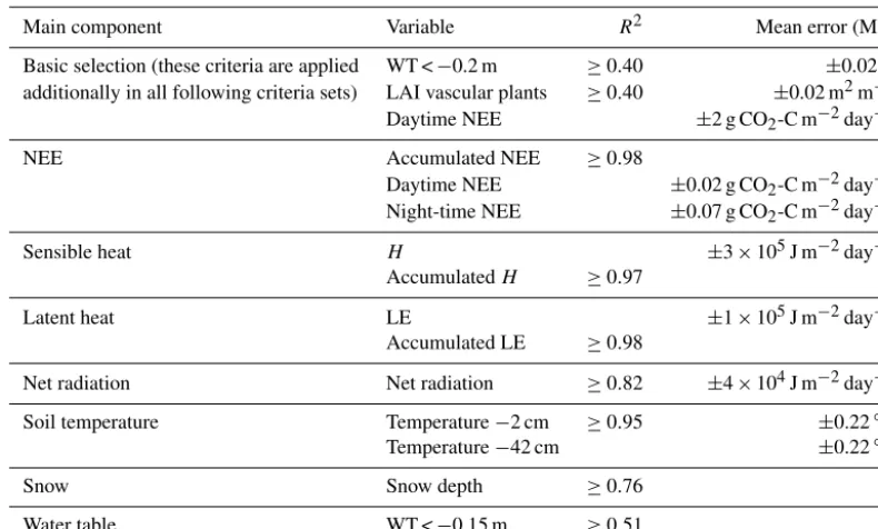
Criteria were applied in two steps. In the first step, a basic set of 1285 behavioural models was selected. Out of these, sev-eral sets of 50 runs each were selected in the second step in two different ways: one for sensitivity analyses and parame-ter ranges, which was based on single criparame-teria, and the other for identification of equifinalities, based on multiple criteria. Basic selection
Table 3.Different criteria sets for the selections of accepted runs.
Main component Variable R2 Mean error (ME) Basic selection (these criteria are applied WT <−0.2 m ≥0.40 ±0.02 m additionally in all following criteria sets) LAI vascular plants ≥0.40 ±0.02 m2m−2 Daytime NEE ±2 g CO2-C m−2day−1
NEE Accumulated NEE ≥0.98
Daytime NEE ±0.02 g CO2-C m−2day−1
Night-time NEE ±0.07 g CO2-C m−2day−1
Sensible heat H ±3×10⁵J m−2day−1 AccumulatedH ≥0.97
Latent heat LE ±1×10⁵J m−2day−1 Accumulated LE ≥0.98
Net radiation Net radiation ≥0.82 ±4×10⁴J m−2day−1 Soil temperature Temperature−2 cm ≥0.95 ±0.22◦C Temperature−42 cm ±0.22◦C Snow Snow depth ≥0.76
Water table WT <−0.15 m ≥0.51
range of daytime NEE ME was additionally applied to ex-clude outliers due to numerical problems, which reached an ME in NEE up to 8×1027g CO2–C day−1m−2in the prior.
Single criteria to identify parameter range
For sensitivity analyses and to test if, and how, parame-ter ranges depend on the selected criparame-teria, the best 50 be-havioural models for each performance index of each vari-able were selected out of the basic selection. Thereby, best means highest in the case of theR2and NSE, but closest to zero in the case of ME. We defined posterior parameter range as the interval between the 5th and the 95th percentile of the distribution of parameter values of the runs selected. Poste-rior parameter ranges were compared with the ranges result-ing from the basic selection. If the upper or lower limit of a posterior parameter range of the final selections differed by ≥10 % from the upper or lower limit of the posterior range of the basic selection, the parameter was assumed to be sen-sitive to the selected criteria and further analysed.
The same was done for each of the best 200 behavioural models, but as the results were similar, they were only plot-ted with respect to parameter ranges. Furthermore, all pa-rameters were plotted against all performance indices of each variable and checked visually for discrepancies with the re-sulting ranges (results are not shown).
Multiple criteria to identify parameter correlations For identification of equifinalities, a set of multiple criteria for each variable (Table 3) was applied to select sets of 50 be-havioural models each. Again, these selections were based on
the basic selection. Parameter ensembles of these accepted behavioural models were then analysed to identify covari-ance between parameters. A pair of parameters was consid-ered to interact if their values correlated with aR2of at least 0.1 in the basic selection, respectively, 0.2 in the final selec-tion. If a pair showed correlations in several criteria sets, the highestR2value was reported in the results.
2.4.4 Evaluation and measures
compared how well overlapping ranges differed between per-formance indices within the same variable and between dif-ferent variables. The overlapping range of each parameter was normalized by dividing it by the average of the poste-rior ranges of this parameter; therefore, a value of 1 would be reached if all posterior ranges of that parameter would be identical for all performance indices and variables. Equifi-nalities were quantified by the R2value of a simple linear regression through the values of the interacting parameter pair in the accepted runs. Parameter concern (P )was defined based on three components: the sensitivity of the parameter, how unambiguously it could be constraint and the sum of correlation coefficients of equifinalities with other parame-ters:
P = SR2+SME
×(1−O)+X2×2
10×R2 equi
10 . (1)
Thereby, sensitivity was the sum of the range reduction for theR2and for ME, respectively NSE in case where no sen-sitivity was detected for the R2 and ME but for the NSE. The sensitivity was multiplied by the factor 1 minus the nor-malized overlapping range, so that the sensitivity of param-eters, which could be unambiguously constrained are down weighted; therefore, with high uncertainty due to different results for different performances, indices or variables are up weighted. Equifinalities were considered by the sum of the R2values for each correlation of that parameter with another parameter, displayed in exponential form and weighted so that strong correlations were emphasized and the contribu-tion of equifinalities were in a comparable scale to the sensi-tivity measures.
3 Results
Processes as well as parameters were strongly interacting, which was reflected in sensitivities of each variable to sev-eral different process categories, correlations between the performance in different variables, and in equifinalities be-tween parameters of different process categories. About half of the parameters were sensitive to model performance in one or more variables, but only a few had a distinct range (Sect. 3.1). Instead they affected several processes, causing trade-offs not only in model performance between the dif-ferent measurement variables and between the difdif-ferent per-formance indices, but also several supporting effects could be identified (Sect. 3.2). A lot of equifinalities were identi-fied between parameters. Parameters were correlated with up to seven other parameters, often from different process cat-egories. Therefore, a good performance often requires cer-tain combinations of parameter values, rather than specific parameter values (Sect. 3.3). Each of the available measure-ment variables (NEE, LAI, sensible and latent heat fluxes, net radiation, soil temperatures, water table depth and snow depth) constrained parameters from several different process
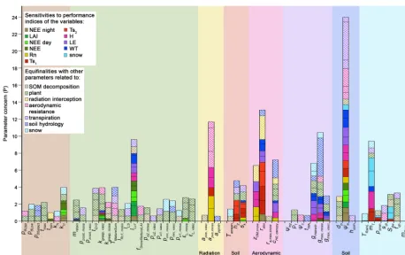
categories, without any variable being redundant (Sect. 3.4). Nevertheless, large uncertainty remained in especially the unsaturated water distribution (ψa)in the soil (Fig. 2), which
affected all considered processes and hindered further param-eter constrain. This might be solved by additional measure-ments of, e.g., soil hydraulic properties. Other important pa-rameters that could not be constrained were the following: define aerodynamic resistance, radiation interception (in par-ticular moss albedo), timing of snowmelt, and in the case of NEE mostly the leaf-litter fall rate of vascular plants during the growing season (Fig. 2). A detailed description of the key parameters for each process and the detected interactions can be found in Sect. 3.5. Results for model fits to the different variables can be found in Fig. S1 in the Supplement. 3.1 Parameter sensitivity
Model performance was sensitive to parameters across the different process categories: out of 27 sensitive parameters 21 affected model performance in more than one variable. For 15 of the sensitive parameters, resulting value ranges dif-fered strongly (less than 50 % overlapping range), depending on both, the variable and the performance index (Fig. S2 in the Supplement). Performance in Ts and WT was determined by 12 key parameters belonging to seven and six different process categories, respectively (Fig. 3). In contrast, snow depth and LAI depended mainly on parameters from their own process categories. Radiation and LAI refer to the sim-plest processes with respect to number of connected param-eters (Fig. 3). However, radiation, together with snow depth, was the variable with the strongest average disagreement in parameter value ranges between the different selection crite-ria (Fig. 4). Four parameters were sensitive to at least half of the considered variables (Fig. 2); the parameter defining the water retention curve and unsaturated soil hydraulic con-ductivity (ψa)affected model performance in variables of all
eight considered variables. The moss transpiration coefficient (gmax,moss), vascular plant respiration coefficient (kgresp,vasc)
and litter fall rate (lLc1)were important parameters for not
only LAI and NEE, but alsoH, LE and WT. Furthermore, gmax,mossandkgresp,vascwere also important for Ts. The
sen-sitivities of the single parameters are described in more detail in Sect. 3.5. The full table of the correlation coefficients be-tween parameters and performance can be found in the Sup-plement (Table S4).
3.2 Confounding and supporting effects of interacting processes
Figure 2.Parameter concern is shown on theyaxis as sum of equifinalities (hatched) and sensitivities that could not be constrained unam-biguously (solid). Thexaxis shows the parameters that belong to the process category of the background colour.
4 6 8 10 12 14 Co un t s en st iv ie p ar am et er s Snow Soil hydrology Transpiration Aerodynamic Parameters belonging to the process category 0 2 4 N EE n ig ht N EE d ay N
EE LAI Rad Ts H LE
W T Sn ow Co un t s en st iv ie p ar am et er s
Variables to which the parameters are sensitive to
Aerodynamic resistance Soil temperature
Radiation interception
Figure 3.Connections between processes and parameters of
differ-ent process categories. The yaxis shows the count of parameters from the different process categories (colours) that are sensitive to model performance in the various variables (xaxis).
accepted value ranges overlapped with 35 % between differ-ent performance indices and between differdiffer-ent sub-periods of the same variable, and additionally with 6 % if the differences between different variables were considered (Fig. 4). In the
0 % 10 % 20 % 30 % 40 % 50 % 60 % 70 % 80 % Av er ag e ov er la pp in g ra ng e -20 % -10 % 0 % N EE n igh t N EE d ay tim e N
EE LAI Rad Ts H LE WT
Sn ow Wi th in p ro ce ss e s Bet w e en p ro ce ss e s To ta l Av er ag e ov er la pp in g ra ng e
Variables to which the parameters are senstive to
Figure 4.Average overlap of accepted ranges per parameter within
each process and between processes, i.e. how unambiguously the parameters could be constrained. Negative values indicate the dis-tance between accepted ranges when ranges did not overlap at all.
case of 11 parameters, the accepted ranges did not overlap at all (Fig. S2 in the Supplement).
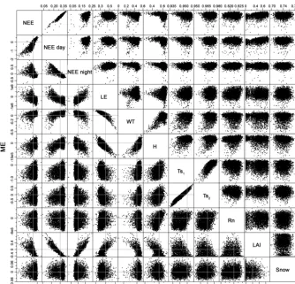
per-Figure 5.Correlations between performance indices in the prior distribution (3200 random runs):R2vs.R2(upper panel); mean error (ME) vs. ME (lower panel). Each of the dots represents a parameter set. Grey lines indicate the axes through zero.
formance in many other variables; the magnitude of vascu-lar plant LAI was strongly correlated with magnitude of LE, WT,H and NEE, especially if daytime and night-time val-ues were considered (Fig. 5). Thereby the lowest ME in day-time and night-day-time NEE, as well as the ME and dynamics of H, went along with a slight underestimation, and for LE and WT with a slight overestimation of vascular plant LAI. The best performance for WT dynamics was reached if the magnitude of vascular plant LAI was correct (Fig. 6). A no-ticeable existence of the vascular plants (LAI ME >−0.4) in-creased the fit in the NEER2to at least 0.2, but this was not a necessary precondition for good NEE performance (Fig. 6). The highest performance in dynamics of WT, H and Ts in the upper layer coincided with a good fit in NEE magnitude (Fig. 6). This relationship was even stronger if these variables were compared to ME in NEE night-time and NEE daytime. A correct representation of WT dynamics and depth coin-cided with high performance inHdynamics and a correct or slightly underestimatedH(Figs. 5 and 6). A small ME inH correlated with high performance in WT dynamics. Perfor-mances in soil temperatures of different layers were strongly correlated with each other in both dynamics and magnitude.
Underestimation of LE was connected to an overestimation ofH, but also to better dynamics inH(Fig. 5). The ME in net radiation was positively correlated with the ME inH. A good fit between modelled and observed snow depth did not cor-relate with the performance in any other variable. The only exception was a negative correlation between the dynamics in snow depth andH if performance during springtime ex-clusively was considered (Fig. S3 in the Supplement).
Especially for snow, Rn and in the case of some parameters also for Ts, accepted ranges were contradictory depending on whether theR2or ME was chosen. In the case of moss albedo (apve,moss)and aerodynamic resistance dependency on LAI
(ralai), the ranges also strongly depended on the season
dur-ing which the variable was considered. For two aerodynamic resistances and one soil parameter (z0M,snow,cH0,canopy,sk)
Figure 6.Correlations between performance indices in the prior distribution (3200 random runs):R2(columns) vs. mean error (ME) (rows). Each of the dots represents a parameter set. Grey lines indicate the axes through zero.
3.3 Equifinalities
Parameters were strongly inter-correlated, often with sev-eral parameters, and often across different process categories. Equifinalities can hinder the identification of sensitivities, which was especially true for the basic selection; despite re-ducing the number of runs by 97.5 %, posterior and prior ranges hardly differed (Table S5 in the Supplement). Instead certain-value triples for photosynthetic efficiency (εL,vasc)
with the respiration coefficient (kgresp,vasc)and with the
stor-age fraction for plant regrowth in spring (mretain)were
cru-cial for the survival of the vascular plant layer. Certain-value pairs for the moss transpiration coefficient (gmax,moss)with
the shape parameter of soil water retention (ψa) were crucial
for a reasonable water table depth.
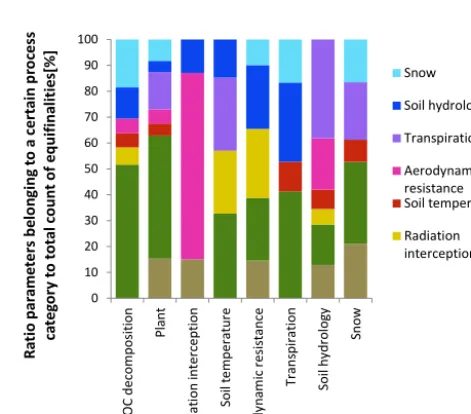
Equifinalities existed not only between parameters from the same process categories, but even more often between parameters from different process categories (Fig. 7). Pa-rameters defining radiation interception, soil temperature, aerodynamic resistance, transpiration, and soil hydrology ex-clusively correlated with parameters from different process categories. Parameters defining radiation interception were
20 30 40 50 60 70 80 90 100 Ra ti o pa ra m et er s be lo ng in g to a c er ta in p ro ce ss ca te go ry to to ta l c ou nt o f e qu ifi na lit ie s[ % ] Snow Soil hydrology Transpiration Aerodynamic resistance Soil temperature Radiation interception 0 10 20 SO C de co m po si tio n Pl an t Ra di at io n in te rc ep tio n So il te m pe ra tu re Ae ro dy na m ic re si st an ce Tr an sp ira tio n So il hy dr ol og y Sn ow Ra tio p ar am et er s be lo ng in g to a c er ta in p ro ce ss ca te go ry to to ta l c ou nt o f e qu ifi na lit ie s[ % ] interception
Figure 7.Process category belonging to parameters that correlated
mostly correlated with parameters defining aerodynamic re-sistance. Only in the case of plant and SOC decomposition parameters, equifinalities existed mainly between parameters of the same process category.
Except forρsmin, all sensitive parameters and other further
parameters were detected to correlate with up to five other parameters in the final selections, ψa correlated with even
seven others (Fig. 2). Two parameters had very strong cor-relations (R2≥0.3) with two other parameters each, which belong to different process categories (ψawithcH0,canopyand
gmax,mossandapve,moss withz0M,snowandralai)(Table S6 in
the Supplement).
3.4 Usefulness of measurement variables
All available measured variables (NEE, LAI, LE, H, Rn, Ts, WT and snow depth) were helpful in constraining pa-rameter ranges (Fig. 2). None of the supporting effects was strong enough, to allow one variable to be fully replace-able by another. Even for the strongest correlation between soil temperatures of the different layers, the remaining un-certainty in one temperature when knowing the other would be of the magnitude of 0.5◦C, which corresponds to more than 25 % of the total uncertainty resulting from the tested parameter ranges (Fig. 5). In the case of 15 variables, the usage of several variables revealed that constrained ranges were not robust. In total, 12 parameters could be unambigu-ously constrained to a more narrow range, as their resulting ranges had at least 50 % overlap, or affected only one vari-able (Fig. S2 in the Supplement). Each varivari-able constrained parameters from several different process categories (Fig. 3). The highest number of correlations was detected for the per-formance in WT and Ts, which constrained 12 parameters from different process categories. Also the available data for LE,Hand NEE constrained many parameters. Nevertheless, large uncertainty remained due to equifinalities and differ-ences in accepted ranges; the largest uncertainty was caused by a parameter defining the shape of the water retention curve (air entry,ψa). As this was the only calibrated parameter of
the water retention curve, it determined the unsaturated hy-draulic conductivity of the soil.ψawas sensitive to all
con-sidered variables and had many strong interactions with other parameters, while it was not possible to constrain it to an un-ambiguous value range (Fig. S2 in the Supplement). There-fore, it would be of great value to be able to deduce such parameters from additional measurements. This also applies to the following parameters, which could not be constrained unambiguously; leaf-litter fall rate of vascular plants dur-ing the growdur-ing season (lLc1) was the second most
sensi-tive parameter, affecting the performance in NEE,H, LE and WT. Moss albedo (apve,moss), aerodynamic resistance
depen-dency on LAI (ralai)and transpiration coefficients (gmax,vasc,
gmax,moss,gmaxwin)had a similar concern, due to their
equifi-nalities to other parameters. Plant respiration (kgresp,vasc)had
strong sensitivity but could be constrained unambiguously by the available data.
3.5 Detailed description of sensitivities and interactions per process
Detected sensitivities, connections between performances, and equifinalities all showed strong interactions between the different processes and parameters of different process cat-egories. Connections existed between all variables and pro-cess categories, but most strongly inter-linked were LE with WT and Rn withHand Ts (Fig. 2).H, LE and WT were also linked to each other and to NEE. The impact of the plant is further reflected in the correlations between performances in LAI with performances in many other variables (Fig. 5). The implications on the performance for each considered variable will be described in the following sections.
3.5.1 Water level depth and soil moisture conditions Performance in water level depth was determined by 12 key parameters (Table S4 in the Supplement). It was most strongly connected to the shape of the soil water reten-tion curve (ψa) as well as to the transpiration coefficients
for mosses and winter transpiration (gmax,moss, gmaxwin).
The transpiration coefficient from vascular plants played a smaller role due to the high sensitivities of parameters defin-ing the growth and therefore the magnitude of the vascular plant (i.e.kgresp,vasc,mretain,lLc1). Equifinalities existed
be-tween several of these parameters.ψahad a strong effect on
the performance of all variables and several strong equifi-nalities, in particular with parameters defining aerodynamic resistance and transpiration. On the other hand, ψa could
not be constrained to an unambiguous range and was there-fore the parameter causing the largest overall uncertainty (Fig. 2). Performance in WT was further sensitive to parame-ters defining aerodynamic resistance, i.e.ralaiandcH0,canopy.
Both parameters had equifinalities withψaand moss albedo
(apve,moss)as well as with timing of snowmelt (mT)and
ther-mal conductivity of snow (sk). In addition, the distance
be-tween drainage (dp)showed some sensitivity.
3.5.2 Transpiration and evaporation
The nine most important parameters for WT performance were also key parameters for LE (ψa, gmax,vasc, gmax,moss,
gmaxwin, kgresp,vasc, mretain, lLc1, ralai, cH0,canopy). This
ex-plains the strong correlation between the performance in WT and LE ME (Fig. 5) and shows the connections with plants, WT and H. Another parameter, sensitive to LE was the roughness length of snow (z0M,snow), belonging to the
its upper range in the case of vascular plants (Fig. S2 in the Supplement). Despite the lower values for mosses, transpi-ration prior to criteria selection was dominated by mosses, due to their higher LAI and coverage (Fig. S4 in the Sup-plement). Crucial for LE performance was also a parameter defining the aerodynamic resistance of the canopy under sta-bile conditions (cH0,canopy): a very small value improved the
R2of LE and spring LE, but downgraded the R2 of accu-mulated LE and of winter radiation. Spring LE was overes-timated in most of the runs (see Fig. S1 in the Supplement). The strongest sensitivity on spring LE was by the coefficient for winter transpiration (gmaxwin): the higher thegmaxwinthe
better theR2and ME. Together with (z0M,snow)this was also
the most important parameter for winter LE. 3.5.3 NEE and LAI
Seven of the nine parameters, which were common for LE and WT, were also among the most effective parameters for NEE (ψa, gmax,moss,gmax,vasc, kgresp,vasc,mretain,lLc1,ralai)
and belong to four different process categories: plant, transpi-ration, soil hydrology and aerodynamic resistance (Table S4 in the Supplement). However, the most sensitive parameter for NEE was the rate coefficient for heterotrophic respiration (kl1), which was especially important for night-time NEE.
Further sensitive parameters for night-time NEE were the growth respiration coefficient for mosses (kgresp,moss)and the
temperature dependency coefficient for heterotrophic respi-ration (tmin. The rates of photosynthesis and its temperature
dependence (εL,vasc,εLmoss,pmn,vasc)were key parameters
for LAI, NEE magnitude or temporal NEE dynamics, respec-tively. Many strong interactions existed between plant pa-rameters, which were especially visible in the basic selection (see Sect. 3.3). The rate of leaf-litter fall during the growing seasonlLc1was one of the parameters with the highest
con-cern, due to its sensitivity on many different processes, its equifinalities and as it could not be constrained to an unam-biguous solution (Fig. 2). Resulting ranges for lLc1differed
not only between the different performance indices within NEE and within LAI, but also between NEE and LAI (Fig. S2 in the Supplement).
3.5.4 Sensible heat fluxes, soil temperatures and net radiation
Many inter-connections existed betweenH, Ts and Rn but all three were also linked with LE, WT, snow and NEE. A snow parameter, determining the timing of snowmelt (mT)was the
most crucial parameter for heat fluxes, not only in springtime but also for the whole year period. Furthermore,mTwas
im-portant for Ts in springtime (see Sect. 3.5.5). The shape of the soil water retention curve (ψa)was the second most
sen-sitive parameter for both variables. The aerodynamic resis-tance dependency factor on LAI (ralai)was the most
sensi-tive parameter for Ts, and affected also LE, WT and
night-time NEE, while it strongly correlated with moss albedo (apve,moss), the third most sensitive parameter forHand most
sensitive parameter for Rn. The accepted ranges forralai
con-tradicted within the soil temperature variables, depending on the chosen performance index and considered season; high values were important for the Ts ME andR2during winter, but low ones improved the TsR2 during spring and during the whole period. Therefore,ralaiwas the parameter causing
the largest overall uncertainty afterψa. This was followed by
apve,moss, which had low values for accepted ranges in the
case ofH, Rn and Ts during the whole period but high val-ues in the case of winterH and Rn. It further showed strong equifinalities with the roughness length of snow (z0M,snow),
which was the second most sensitive parameter for Rn, but also affected H and LE. The coefficient for thermal con-ductivity of snow (sk)affected Rn and Ts but not H. The
thermal conductance coefficient of soil organic material (h2),
the lower boundary mean temperature (Tamean), the snowmelt
dependency to radiation coefficient (mRmin)and the density
of new and old snow (ρsmin,Sdw)affected only soil
temper-atures, the latter two also snow depth. Parameters defining moss and winter transpiration (gmax,moss, gmaxwin)and the
growth respiration coefficient of vascular plants with its ef-fect on vascular plant biomass and LAI (kgresp,vasc)were
sen-sitive to Ts,gmax,mossandkgresp,vascas well as toH. The most
important parameter for LE,cH0,canopywas another key
pa-rameter for Rn andH. 3.5.5 Snow
The temperature coefficient in the snowmelt function (mT)
was the most important parameter for ME in snow and deter-mined the timing of snowmelt. However, resulting parame-ter ranges did not overlap between the different performance indices within the snow-depth variable and between differ-ent other variables. A longer lasting snow cover (lowmT< 3)
was crucial for spring H and reduced mean error in snow depth, but loweredR2values in spring Ts and snow depth. mTinteracted with another snow parameter (TRainL)as well
as with parameters from the temperature and transpiration process category (Tamean,gmaxwin). The density coefficients
for old (Sdw)and new snow (ρsmin)had medium effect on
snow-depth performance and also affected spring and winter soil temperatures in all layers, but the latter could be unam-biguously constrained by the available data.
4 Discussion
(SOC decomposition, plant growth-related processes, radia-tion intercepradia-tion, soil temperature, aerodynamic resistance, transpiration, soil hydrology and snow) in a peatland ecosys-tem. Similar to results from a forest modelling study using the DRAINMOD-Forest model (Tian et al., 2014) and a N2O
study using the CoupModel on a drained peatland forest (He et al., 2016), we found that processes were sensitive to pa-rameters from several different process categories. Together with the discovered supporting effects between model per-formances in different variables, this confirms the connec-tions and dependencies between different processes as im-plemented in the model (see “Model description and equa-tions”, Sect. 2.3, Table 2 in the Supplement and Janson and Karlberg, 2010). The many equifinalities within and between different process categories reveal the dependency of con-strained parameter ranges as well as parameter sensitivities to model structure, calibration set-up and parameters with fixed values; a deviation in one of these factors leads to dif-ferent optimal value ranges, whereas a non-sensitive param-eter might become sensitive if an interacting paramparam-eter is set constant. This implies a limited transferability of parameter values between models in general and even between studies using the same model in a different configuration. Resulting parameter ranges were moreover affected by the applied cri-teria for selecting runs. Yet, it is quite common practice to adopt at least some parameter values from other modelling studies (e.g. Frolking et al., 2002, Yurova et al., 2007; St-Hilaire et al., 2010; Wania et al., 2010; Gong et al., 2013; Kim et al., 2014; Kurnianto et al., 2014; Zhu et al., 2014), which includes the usage of model default values that were estimated under a different model configuration.
The strong interactions across different process categories also emphasize the importance of measurements of ancillary data additionally to the variable of interest and model input data (meteorological and SOC data). Measurements of NEE, LAI, LE,H, Rn, Ts, WT and snow were all found to be valu-able for constraining parameters from several different pro-cess categories and can therefore reduce uncertainty in model predictions. Further constraint of the parameters in this study would be possible if especially additional water content or soil hydraulic properties were measured.
Beside parameter uncertainty, also uncertainty in model structure and in measured input and calibration data con-tribute to model uncertainty (Thorsen et al., 2001; Beven and Freer, 2001). This was tested for other peatland models (e.g. model structure: Tang et al., 2015; input drivers: Wania et al., 2009; St-Hilaire et al., 2010; Grant et al., 2011; Kim et al., 2014), but goes beyond the scope of this study. Here, only one model and one site were investigated. A previous study using CoupModel investigated the differences of parameter ranges between several different peatland sites (Metzger et al., 2015).
4.1 Parameter sensitivity
The sensitivity of variables to parameters from many dif-ferent processes revealed the importance of process interac-tions. Especially abiotic processes were strongly inter-linked, but also biotic variables showed sensitivities to parameters from up to seven different process categories, suggesting that parameter sensitivities and model performance of a certain process depend on which other process categories are con-sidered in a model and in a calibration. This is an important finding, as many studies investigate the sensitivity of often only a few parameters from mainly the same process cate-gory as the output variable (e.g. Yu et al., 2001; Frolking et al., 2002; Belassen et al., 2010; Wania et al., 2010; Morris et al., 2012; Wu and Blodau, 2013; Zhao et al., 2014; Zhu et al., 2014), which might lead to sensitivities and resulting ranges that are not robust. The identified interactions can help mod-ellers to develop or select an appropriate model including the parameters, processes and process categories that need to be considered together, depending on the variable of interest.
prior distributions of the parameters (e.g. Tatarinov and Cien-ciala, 2006). Furthermore, our results have shown that the pa-rameter ranges depend on model structure, on the selection of parameters for calibration and on the selected acceptance criteria. Thereby, not only the selected variable but also the selected sub-period was relevant, as has been shown by other studies as well (e.g. Prihodko et al., 2008; Van Huisteden et al., 2009; Safta et al., 2015).
4.2 Confounding and supporting effects of interacting processes
Criteria selection is a subjective choice of the modeller if multiple output variables are available. The identified sup-porting effects and trade-offs between the performances in different variables allow modellers to assess the implica-tions of a certain criteria on model performance and param-eter ranges and to choose criteria according to the processes of interest; however, some of them might be ecosystem or model specific. Trade-offs existed not only between differ-ent variables but also within the same variable, depending on whether ME, R2 of actual orR2 of accumulated values were chosen and which season was considered. This implies that the problems of a subjective criteria selection also exist if only one time series variable is considered. Even if a stan-dardized multi-criteria optimization algorithm like Bayesian calibration or a more sophisticated performance index com-bining several performance measures is used, the choices and the corresponding weightings are moved to the developer of the algorithm or index, but still remain subjective.
More than half of the sensitive parameters in this study could not be constrained to an unambiguous range. Con-straining such a parameter by only one variable and one in-dex would result in a range that is not robust. Using sev-eral measurement variables and sevsev-eral indices can therefore help to test the robustness of calibrated parameters. A pa-rameter that is robust might better represent a physical con-stant, whereas controversial resulting ranges might hint at a not well represented system; there is no value for this pa-rameter that leads simultaneously to the best performance for dynamics and magnitude in all variables and during all periods. Instead of a physical constant this parameter might correspond to a dynamic process. Beside model inadequacy, mismatching ranges could be caused in some cases by an in-appropriate performance index (see discussion in Sect. 4.5.4) or measurements that do not truly represent the modelled variable. For example, with the EC technique, NEE is not di-rectly measured as the CO2exchange between biosphere and
atmosphere at a certain point, but rather results from calcu-lations of the turbulent exchange of vertical fluxes measured several metres above the ground. Moreover, fluxes may orig-inate from a footprint area that changes diurnally and sea-sonally and thus may include different soil conditions and vegetation.
Usually, LE is assumed to be closely connected to NEE due to the coupling of transpiration and carbon assimilation in vascular plants (e.g. Schulze, 2006), but has also been shown to correlate for mosses (e.g. Robroek et al., 2009). Our study reveals much stronger relations between parame-ters definingHand NEE, than between LE and NEE. Trade-offs between performance in LE and NEE were also found by Staudt et al. (2010) and Prihodko et al. (2008) in a forest and a forest complex including wetlands. However, only the effect of parameters, not the effect of model input (i.e. mete-orological input data), on these processes were tested in both studies, as well as in ours. Such a confounding effect might also result from a parameter value compensating for a pro-cess not implemented in the model. For example, parameter values that lead to an overestimation of NEE in spring result in higher transpiration and therefore better LE, whereas the reason for the underestimated LE during April to mid-June (Fig. S1 in the Supplement) might in fact be caused by evaporation from open water bodies that form on the peatland during spring and early summer, a process not implemented in the applied version of CoupModel.
4.3 Equifinalities
The fit of model output to measured data in complex models is often not driven by a particular parameter but instead by interactions among parameters (e.g. Beven and Freer, 2001), which was also the case for several parameters in our study, hindering the constraint of parameters to a more narrow range. Furthermore, other carbon modelling studies found that parameter values and sensitivities depend on the val-ues of other parameters (e.g. Tatarinov and Cienciala, 2006; Verbeeck et al., 2006; Quillet et al., 2013). This implies that especially if only a few parameters and processes are cali-brated (as in e.g. Yu et al., 2001; Wania et al., 2010, Zhu et al., 2014; Kim et al., 2014, Tang et al., 2015), resulting constrained ranges might not be comparable and transferable between models differing in their constant parameter values. Many equifinalities were identified, not only between param-eters from the same process category but also across differ-ent process categories. This means that the problem of lim-ited transferability also applies if parameters from only one process category are calibrated (as e.g. in Wang et al., 2005; Belassen et al., 2010; Wania et al., 2010; Sándor et al., 2016) or if models differ in the structures and implementations of their modules. The knowledge on equifinalities is needed for a better parameter constraint in future calibrations as it al-lows for calibration of the connected parameters dependent on each other. Another way to respond to identified equifi-nalities is to calibrate only one of the connected parameters. However, the resulting range will then not be transferable to other models using different values for connected, constant parameters.
Some equifinalities included several parameters, making their visualization impossible and simple regression an in-sufficient tool for fully detecting and describing them (see Saltelli et al., 2008). These equifinalities need to be further investigated in additional calibrations that incorporate those parameter interactions and constrained ranges, which were unambiguous, to achieve a higher number of acceptable runs. This is needed, because the numbers of accepted runs in the final selections (50) did not allow for a much more detailed analysis in such a complex model, as was apparent in com-parison with the basic selection; aR2threshold value of 0.1 was sufficient to identify equifinalities in the basic selection of 1286 accepted runs, but with just 50 accepted runs in the final selections; this threshold value could easily be exceeded by a random distribution, even when a higher threshold value of 0.15 was used. A threshold of 0.15 was, on the other hand, already too high to detect, for example, the strong relation-ships between the plant parameters that were only clearly vis-ible in the basic selection. Nevertheless, the six equifinalities with aR2of higher than 0.30 are unambiguous in this appli-cation of the CoupModel and those with lower values are still very useful to design future calibrations to further investigate and describe these equifinalities.
4.4 Usefulness of measurement variables
Models can be improved and their uncertainty reduced by calibrating their parameters to measurement data (e.g. Friend et al., 2007; Wang et al., 2009; Williams et al., 2009). We tested the potential of several measurement variables (NEE, LAI, LE,H, Rn, Ts, WT and snow depth) and found that all contributed to a better parameter constraint.
Thereby none of the variables could be fully replaced by another. Due to the strong interactions and as parameters of each process category were constrained by several different variables, ancillary variables are valuable even if only one certain process is of interest. In the case of snow, our results suggest that data on snow cover might be sufficient if snow depth is not available.
In a forest site simulation with the ORCHIDEE model,H and Rn were found to be redundant for constraining energy balance parameters if NEE and LE were available (Santaren et al., 2007). In contrast, some energy balance-related pa-rameters in our study were constrained exclusively by Rn andH, or additionally by LE, but with different resulting ranges. This reveals the usefulness of Rn andH measure-ments for model constraints, and shows that variables which might have been identified as redundant in one study could be of high importance on another ecosystem or for another model calibrating a different parameter selection.
Several influential parameters could not be unambigu-ously constrained or showed equifinalities and need addi-tional measurements to be further investigated. This includes soil water content or soil water retention properties, as well as canopy albedo and leaf-litter fall during the growing sea-son. Except for water retention properties these variables are needed as time series throughout the year. A more detailed discussion of the benefit of such measurements can be found in the following sections.
4.5 Detailed discussion of sensitivities and interactions per process
The parameters that were identified as most influential or that showed the strongest equifinalities were related to soil hydrology and water content, to a stable representation of the plant, to radiation, temperature and heat fluxes or to snow. As only one parameter per equation was calibrated, a high sensitivity to this parameter means a high sensitivity to the corresponding process. Some of such process sensi-tivities might also be interesting for other models and similar ecosystems. The introduced index to measure parameter con-cern includes subjective choices such as weighting factors, the choice of considered calibration variables and their sub-periods as well as the chosen performance indices. However, several tested variations in especially the weighting did not noticeably change the results;ψa was always the most