www.geosci-model-dev.net/8/2627/2015/ doi:10.5194/gmd-8-2627-2015
© Author(s) 2015. CC Attribution 3.0 License.
Methods for automatized detection of rapid changes in lateral
boundary condition fields for NWP limited area models
M. Tudor
Meteorological and Hydrological Service, Griˇc 3, Zagreb, Croatia Correspondence to: M. Tudor ([email protected])
Received: 12 January 2015 – Published in Geosci. Model Dev. Discuss.: 10 March 2015 Revised: 29 June 2015 – Accepted: 2 August 2015 – Published: 24 August 2015
Abstract. Three-hourly temporal resolution of lateral bound-ary data for limited area models (LAMs) can be too infre-quent to resolve rapidly moving storms. This problem is expected to be worse with increasing horizontal resolution. In order to detect intensive disturbances in surface pressure moving rapidly through the model domain, a filtered sur-face pressure field (MCUF) is computed operationally in the ARPEGE global model of Météo France. The field is dis-tributed in the coupling files along with conventional meteo-rological fields used for lateral boundary conditions (LBCs) for the operational forecast using limited area model AL-ADIN (Aire Limitée Adaptation dynamique Développement InterNational) in the Meteorological and Hydrological Ser-vice of Croatia (DHMZ). Here an analysis is performed of the MCUF field for the LACE coupling domain for the pe-riod from 23 January 2006, when it became available, un-til 15 November 2014. The MCUF field is a good indica-tor of rapidly moving pressure disturbances (RMPDs). Its spatial and temporal distribution can be associated with the usual cyclone tracks and areas known to be supporting cy-clogenesis. An alternative set of coupling files from the IFS operational run in the European Centre for Medium-Range Weather Forecasts (ECMWF) is also available operationally in DHMZ with 3-hourly temporal resolution, but the MCUF field is not available. Here, several methods are tested that detect RMPDs in surface pressure a posteriori from the IFS model fields provided in the coupling files. MCUF is com-puted by running ALADIN on the coupling files from IFS. The error function is computed using one-time-step inte-gration of ALADIN on the coupling files without initializa-tion, initialized with digital filter initialization (DFI) or scale-selective DFI (SSDFI). Finally, the amplitude of changes in the mean sea level pressure is computed from the fields in the
coupling files. The results are compared to the MCUF field of ARPEGE and the results of same methods applied to the coupling files from ARPEGE. Most methods give a signal for the RMPDs, but DFI reduces the storms too much to be detected. The error functions without filtering and amplitude have more noise, but the signal of a RMPD is also stronger. The methods are tested for NWP LAM ALADIN, but could be applied to other LAMs and benefit the performance of cli-mate LAMs.
1 Introduction
Operational lateral boundary conditions (LBCs) are provided to limited area models (LAMs) at a time interval of sev-eral hours, referred to as the coupling update period. These data are used at lateral boundaries of the LAM domain every LAM time step of several minutes. Consequently, LBC data of the large-scale model are (linearly) interpolated in time. The interpolation procedure distorts the model fields and can lead to LAM forecast failures in the case of fast propagating storms. The problem of linear interpolation of model fields in time for cases with rapidly moving storms that enter the LAM domain is expected to become worse as both global models and LAMs move to higher resolutions. These storms are associated with rapidly moving pressure disturbances that will be referred to as RMPDs in this text. The problem could be even more pronounced in climate LAMs that couple to large-scale data that are available with a longer interval.
lateral boundaries through the domain during the forecast time (Nicolis, 2007); these errors amplify and spread further with longer time of integration (Nutter et al., 2004). A large LAM domain was recommended (Staniforth, 1997) to pre-vent boundary-induced errors from propagating to the area of interest. However, there are problems that can not be cured by making the LAM domain larger (Vánnitsem and Chome, 2005). For an overview of issues related to LBCs, see Warner et al. (1997).
Regional climate models are expected to develop small-scale features due to high-resolution surface forcings, non-linearities in atmospheric dynamics and hydrodynamic stabilities (Denis et al., 2002). A large coupling update in-terval can make LBCs act as a filter of small-scale features that (should) enter the LAM domain. Climate LAMs without small-scale information in the initial conditions and LBCs develop small-scale variance even in the absence of surface forcing due to non-linear cascade of variance (Laprise et al., 2008), but it takes several days.
Currently, there are two sets of LBC data that can be used for operational forecast using the ALADIN (ALADIN International Team, 1997) (Aire Limitée Adaptation dy-namique Développement InterNational) LAM in the Mete-orological and Hydrological Service of Croatia (DHMZ). One is from the global Integrated Forecast System (IFS) of the European Centre for Medium-Range Weather Forecasts (ECMWF) and another is from the Action de Recherche Petite Echelle Grande Echelle (ARPEGE; see e.g. Cassou and Terray, 2001) global model of Météo France. The LBCs from the global numerical weather prediction (NWP) models ARPEGE and IFS are operationally provided with a 3 h in-terval. These are used for running the operational ALADIN forecast in 8 km resolution (Tudor et al., 2013). Coupling is performed along the lateral boundaries in the eight grid points from domain edge by means of the Davies (1976) cou-pling scheme and by using linear interpolation in the time of the input fields from the global model.
Termonia (2003) has analysed the Lothar storm (Wernli et al., 2002) and found that the 3-hourly coupling update inter-val is insufficient for resolving the storm in lateral bound-aries. Also, Davies (2014) finds that 3-hourly LBCs lose in-formation for a 12 km resolution LAM coupled to a 12 km resolution large-scale model (see Fig. 5c in Davies, 2014). In order to monitor the occurrence of potential LAM fore-cast failures due to insufficient coupling update frequency, a recursive high-pass filter (Termonia, 2004) has been im-plemented in the ARPEGE model and applied to the surface pressure field. The filtered surface pressure field is referred to as the monitoring of the coupling update frequency (MCUF) field. Large values of the MCUF field indicate a RMPD in the surface pressure through that model grid point. A value larger than a threshold value suggests that a fast cyclone has moved through the area.
The MCUF field has been provided since the 06:00 UTC run on 23 January 2006 in the coupling files from global
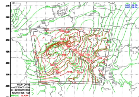
Figure 1. Mean sea level pressure (hPa)from ARPEGE (green) and ALADIN (red) operational 60 hour forecast starting from 12 UTC analysis on 27thOct 2008. The coordinates and values of MCUF field exceeding the 0.003 threshold are listed in the upper right corner and plotted as blue dots on the map.
Warner, T., Peterson, R., and Treadon, R.: A tutorial on lateral boundary conditions as a basic and potentially
695
serious limitation to regional numerical weather prediction. Bull. Amer. Meteor. Soc., 78, 2599–2617, 1997. Wernli, H., Dirren, S., Liniger, M.A., and Zillig, M.: Dynamical aspects of the life cycle of the winter storm
Lothar (24–26 December 1999). Q. J. R. Meteorol. Soc., 128, 405–429, 2002.
Žagar, N., Honzak, L., Žabkar, R., Skok, G., Rakovec, J., and Ceglar, A.: Uncertainties in a regional climate model in the midlatitudes due to the nesting tecnique and the domain size, J. Geophys. Res. Atmos., 118,
700
6189–6199, 2013.
22
Figure 1. Mean sea level pressure (hPa) from ARPEGE (green) and
ALADIN (red) operational 60 h forecast starting from 12:00 UTC analysis on 27 October 2008. The coordinates and values of the MCUF field exceeding the 0.003 threshold are listed in the upper right corner and plotted as blue dots on the map.
model ARPEGE, run operationally in Météo France, for the common coupling domain used for LBC data in six coun-tries (Austria, Croatia, Czech Republic, Hungary, Slovakia and Slovenia). This common domain will be referred to as the LACE (Limited Area for Central Europe) domain. The horizontal resolution of the LACE coupling domain provided from ARPEGE has changed over the years (see Table 1), but the aerial coverage of the LACE coupling domain provided from ARPEGE remained the same (see the aerial coverage of the green isolines in Fig. 1). Local operational domains are smaller than the LACE domain, but have higher horizon-tal resolution and have coupling zones eight grid points wide along lateral boundaries. If the point with the large MCUF value is inside the coupling zone of the ALADIN domain, it can be expected that the ALADIN model run will miss the cyclone strength due to interpolation of boundary data in time. These events are expected to be rare, at least ac-cording to the analysis performed on 1 year of data for the Belgian domain (Termonia et al., 2009). But rapid changes in surface pressure are associated with the most intensive storms moving rapidly, pose a threat to the public and require warning. It is very important that operational NWP models forecast such events. The frequency of such events is anal-ysed for the LACE domain on almost 9 years of data from the operational ARPEGE fields (from 23 January 2006 until 15 November 2014).
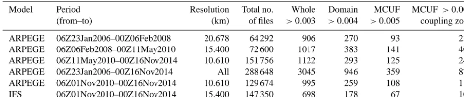
Table 1. Model, period, horizontal resolution and total number of the coupling files for which the rapid changes in the surface pressure
field were analysed; the field used was received from Météo France and computed by ALADIN for files received from ECMWF. The rapid changes in surface pressure for the first 3 h were omitted from the analysis due to evidence of model spin-up for some periods.
Model Period Resolution Total no. Whole Domain MCUF MCUF >0.003
(from–to) (km) of files >0.003 >0.004 >0.005 coupling zone
ARPEGE 06Z23Jan2006–00Z06Feb2008 20.678 64 292 906 270 93 235
ARPEGE 06Z06Feb2008–00Z11May2010 15.400 72 600 1017 383 141 400
ARPEGE 06Z11May2010–00Z16Nov2014 10.610 151 756 1122 293 125 243
ARPEGE 06Z23Jan2006–00Z16Nov2014 All 288 648 3045 946 359 878
ARPEGE 06Z01Nov2010–00Z16Nov2014 10.610 129 674 995 259 108 186
IFS 06Z01Nov2010–00Z16Nov2014 15.400 147 350 698 178 67 109
in roughly 16 km resolution and LAM in 8 km resolution, then hourly data would be less satisfactory when both global model and LAM move to higher resolutions (as was already announced at various meetings in 2014). Also, running old cases from stored archive data requires using LBCs with a 3 h interval.
There are other solutions proposed to solve the problem of errors in LBCs caused by time interpolation of fields. The first one (Termonia et al., 2009) is to restart the model fore-cast from the coupling file when the storm is inside the do-main using the scale-selective digital filter initialization (Ter-monia, 2008). The second one is to insert the storm by means of grid-point nudging (Termonia et al., 2011). Both of these require one to stop the model run, insert the storm artificially and continue the model run from there. Using corrected in-terpolation with time derivatives (Termonia, 2003), Boyd’s periodization method (Boyd, 2005; Termonia et al., 2012) can also improve the forecast (Degrauwe et al., 2012), and alternative methods of interpolating LBC data in time (Tudor and Termonia, 2010) do not require restarts, but are compu-tationally expensive, so these would also be used only when needed. However, in order to apply any of these solutions, we should first detect the RMPD in the fields used on lateral boundaries.
Using MCUF implies that the global model computes it operationally and distributes the field in the output files to-gether with the other forecast fields. However, LAM can be coupled to various global model forecasts or larger-scale LAMs for operational forecast and re-analyses for climate model studies or simulations of specific phenomena. With the exception of ARPEGE, global models do not provide a field that would diagnose rapid changes in pressure that occurred in each grid point during a time interval between two con-secutive output files. The centres that provide global model fields could be discouraged from computing an MCUF field due to the computational cost and potentially complex imple-mentation in the model code, and especially from re-running the re-analysis cycles to provide such data for studies of his-torical weather. It is therefore useful to detect RMPDs a pos-teriori using the standard meteorological fields usually pro-vided in model output. The method should enable automatic
detection of a RMPD to be useful in the operational forecast as well as in the climate simulations using LAM. As pointed out by the reviewers, fast-moving disturbances in the upper layers of the atmosphere or inertia-gravity waves are more common. These are also a source of error in LAMs while MCUF detects disturbances in the surface pressure. The fo-cus of this article are rapidly moving disturbances in surface pressure, but a method that detects them could be applied to an upper-level field.
LAMs used for simulations of climate use input LBCs that are available in a coupling update interval of 3 h or more. Simultaneously, LAMs tend towards higher horizontal res-olutions. A number of climate studies have been performed (Horvath et al., 2011; Hamdi et al., 2012; De Troch et al., 2013; Hamdi et al., 2014) using ALADIN in combination with ERA40 (Uppala et al., 2005) and ERA-Interim (Dee et al., 2011) data sets for LBCs. These applications would also benefit from a method that would detect RMPDs a posteriori from the standard meteorological fields used for LBC.
The NWP suite at DHMZ is focused on forecasting weather in the area of Croatia. Cyclones that affect that area often originate from the western Mediterranean and the Adri-atic (Horvath et al., 2008, 2009), which is recognized as a particularly active region with respect to cyclones (Campinis et al., 2000; Alpert et al., 1990). Severe precipitation events occur when a cyclone produces convergence of the moist air and a large quantity of precipitable water (Lionello et al., 2006). The western Mediterranean experiences flash flood events that arise from extremely high rainfall rates (Doswell et al., 1996).
running ALADIN for one time step. The error was estimated for surface pressure and mean sea level pressure using cou-pling data without initialization, or initialized to remove the high-frequency noise. Additionally, this work proposes to es-timate the magnitude of pressure variations by computing a simple amplitude of oscillations between the successive cou-pling files.
The next section describes the models briefly, the methods used to detect RMPDs and the effect of linear interpolation in time on mean sea level pressure. The analysis of 9 years of the MCUF field from ARPEGE is presented in Sect. 3. Re-sults of methods for detecting RMPDs in IFS coupling fields are presented in Sect. 4. The last section gives conclusions.
2 Model description and methods of detection of rapidly moving pressure disturbances
2.1 Operational forecast model
ALADIN is used for operational weather forecast in DHMZ in 8 km resolution using hydrostatic dynamics and two-time-level semi-implicit semi-Lagrangian and stable extrapolation two-time-level schemes (Hortal, 2002). Operationally, the model uses 37 levels in the vertical and a mass-based hybrid terrain-following vertical coordinate η (Simmons and Bur-ridge, 1981).
The initial conditions for the operational forecast are ob-tained using the data assimilation procedure (Staneši´c, 2011). Details of the operational forecast suite as well as model set-up are provided in Tudor et al. (2013), but there were few changes. The forecast is run up to 72 h four times a day, start-ing from the 00:00, 06:00, 12:00 and 18:00 UTC analyses, and coupled to LBC fields from IFS in delayed mode. This means that the LBC for the 6 h forecast from the 18:00 UTC run of IFS is used for the initial LBC for the 00:00 run of the next day, the 9 h forecast from the 18:00 UTC run of IFS is used for the 3 h forecast LBC for the 00:00 run of the next day, and so on.
The 8 km resolution operational forecast is coupled to a global model on the eight-point wide zone along lateral boundaries using the relaxation technique (Davies, 1976) and linear interpolation of LBC data in time (Haugen and Machenhauer, 1993; Rádnoti, 1995). Each coupling file con-tains the complete set of fields needed to initialize the AL-ADIN model forecast.
Digital filter initialization (DFI) is implemented in AL-ADIN in order to remove high-frequency noise (Lynch and Huang, 1992) that arises due to interpolation of the coupling fields from the global model grid to the grid of the cou-pling files and then again to the resolution of the LAM (and changes in the height of the topography in different mod-els/resolutions). Since DFI can considerably reduce the depth of the RMPD due to the Doppler effect, alternative scale-selective digital filter initialization (SSDFI) was proposed,
implemented and tested in the ALADIN model (Termonia, 2008).
2.2 Global model ARPEGE
ARPEGE is a global semi-Lagrangian spectral model run op-erationally at Météo France on a stretched and rotated grid (Courtier and Geleyn, 1988) with highest horizontal resolu-tion over France and lowest resoluresolu-tion on the opposite side of the Earth. The horizontal resolutions in the model fore-cast and data assimilation procedure were changing during the 9 years when the MCUF field was computed in the op-erational ARPEGE forecast. The horizontal resolution of the coupling files also changed twice: see Table 1.
ARPEGE can use coarser resolution in the variational data assimilation procedure than in the forecast run. The fields from the operational forecast are interpolated from the stretched and rotated native model grid to the grid of the lim-ited area LACE domain in Lambert projection of the cou-pling files.
The fields from operational ARPEGE forecasts are avail-able in the coupling files with a 3 h interval for 4 runs per day (starting from the 00:00, 06:00, 12:00 and 18:00 UTC analyses) and extending up to 72 for the 00:00, 06:00 and 12:00 UTC runs and up to 60 h for the 18:00 UTC run. ARPEGE computes the MCUF field operationally according to Termonia (2004) and the field is distributed in the coupling files.
2.3 Global model IFS
IFS is also a global spectral model that uses semi-Lagrangian advection. It is run operationally at ECMWF with uniform horizontal resolution over the globe. The details of the op-erational set-up in the model forecast and data assimilation have changed over the years used for this study, while the LBC files were available operationally, as were the opera-tional model versions. The model forecast fields are interpo-lated from the IFS model grid to the LAM grid in Lambert projection and the horizontal resolution of the coupling files remained 15.4 km (see Table 1).
Following the research studies where LBC data from IFS have been used for studies of severe weather cases (Ivatek-Šahdan and Ivanˇcan-Picek, 2006; Brankovi´c et al., 2007, 2008), the operational forecast run of the ALADIN model in DHMZ has switched to using LBC data from IFS on 1 Jan-uary 2014.
The MCUF field is not computed by the IFS operational suite and is therefore not available in the coupling files from IFS provided by ECMWF. Rapid changes in the surface pres-sure or the mean sea level prespres-sure were detected in the fields provided from IFS operational forecast in the coupling files on the LACE common domain using a number of tools.
the MCUF field was computed during the model run. The computed MCUF field will be referred to as IFSM. However, this means that a different model was run (ferent dynamics and physics) and the results can be dif-ferent than when computed in the host model.
– The error function from Termonia (2003) was computed by running a one-time-step forecast starting from fields in the coupling files (in the same horizontal and vertical resolution); three sets of experiments were performed using initialization without filtering, using DFI or SS-DFI.
– The amplitude of the oscillations in the surface pressure (and mean sea level pressure) was computed from three consecutive coupling files.
The last item actually detects situations when the moving pressure disturbance would be missed using the 21t (6 h) coupling update interval and not the 1t (3 h) interval. But the large values of this field can mean that the interval as short as1tcan also be insufficient for proper representation of lateral boundary data by linear interpolation of the LBC fields in time.
2.4 Computing the monitoring of the coupling update frequency (MCUF) field from the ECMWF coupling files
ALADIN can compute the MCUF field during the model forecast. The field was computed by running ALADIN on the LACE domain of LBC files from operational IFS with a horizontal resolution of 15.4 km (the same resolution and grid as the coupling files) and a time step of 600 s. The output IFSM field is written with a 3-hourly interval. The same pro-cedure has been performed on the LBC files provided from 27 October 2010 until 15 November 2014, for four runs per day (starting from the 00:00, 06:00, 12:00 and 18:00 UTC analyses) and extending to the 78 h forecast.
The maximum value of the IFSM field on the domain cov-ered by the coupling files has been computed for each fore-cast output file. The average IFSM has been computed, the number of files when it exceeded the critical value and the maximum value achieved in each grid point for the coupling files for a 6 h forecast and longer.
The same procedure applied to the ARPEGE coupling files
MCUF was also computed by running ALADIN on the domain and at the resolution of the coupling files from ARPEGE and this field is referred to as the ARPM field to distinguish it from the MCUF field computed in the ARPEGE forecast. But the coupling files from the ARPEGE global model are provided in different horizontal resolutions than the files from IFS. There was no period when both cou-pling files used the same horizontal resolution (Table 1). It is
more important to test the method on both sets of coupling files on the same period in time since the frequency of the occurrence of the fast storms can have significant seasonal and annual variability.
2.5 The error function
Each coupling file contains the complete set of model fields that can also be used as an initial file to perform a forecast run using the ALADIN model. The coupling data are used as initial fields to perform a model integration of one time step forward in time in order to obtainF (t+δt )and the ten-dencies of the model variables. In order to avoid spurious high-frequency noise, a filter initialization should be applied before the start of the model run.
When investigating the error due to linear interpolation of surface pressure, Termonia (2003) computes an error func-tion from the surface pressure field and finds that its maxi-mum over the model domain is a good indicator of a RMPD. Each coupling file contains the complete set of fields needed to initialize the model, so they can be used as initial fields to perform one-time-step model integration. Termonia (2003) defines a dimensionless estimate of the truncation error due to linear interpolation in time as
eT = 1 4
F0(t2)−F0(t1)(t2−t1)
F (t1)+F (t2) , (1)
whereF (t1,2)are the values of the model fieldF at times
when the LBC data are available in the coupling files and
t2−t1is therefore the coupling update interval (3 h).F0(t1,2)
is the tendency of the fieldF at time t1,2 and can be
com-puted asF0(t1,2)=F (t1,2
+δt )−F (t1,2)
δt , where δt is the model time step. The error function of surface pressure and mean sea level pressure was computed for each coupling file. The tendencies can be computed without any filtering of the field in coupling files, using DFI (Lynch et al., 1997) or SSDFI (Termonia, 2008).
The error functioneT has been computed for the surface pressure field from IFS coupling files. The maximum values over the model domain are
ET =max(eT(x, y)) , (2)
whereeT is the error computed in each grid point.
2.5.1 Digital filter initialization
Coupling files contain already interpolated data (to a Lam-bert conformal grid), not the data from the native global model grid. Horizontal interpolation of the surface pressure field (and other forecast fields) from native IFS grid and to-pography to the grid and toto-pography of the LBC files also distorts the fields, so there could be spin-up when comput-ing the tendencies. This change in geometry can generate high-frequency noise that can be removed using DFI (Lynch and Huang, 1992). The DFI was applied using a Dolph– Chebyshev filter on 14 time-step adiabatic backward integra-tion and 14 time-step forward integraintegra-tion with a time step of 600 s. The time span was 2.333 h and the stop band edge period was 3 h; the ripple ratio 0.05 yields a minimum time span of 2.07 h (Lynch, 1997) used with the scheme for dia-batic DFI in ALADIN (Lynch et al., 1997).
2.5.2 Scale selective digital filter initialization
The Doppler effect can shift the frequencies of RMPDs into the range of spurious gravity waves that DFI was designed to remove. Consequently, DFI reduces the intensity of RM-PDs (Termonia, 2008). Alternative SSDFI is expected to be a better solution for initializing the fields used to compute the error function intended to detect RMPDs.
The SSDFI was applied using the Dolph–Chebyshev filter on time-step adiabatic backward integration and eight-time-step forward integration with a time step of 600 s. The time span was 1.333 h, the stop band edge period was 1.5 h, the ripple ratio 0.05 yields a minimum time span of 1.019 h and the cutoff frequency increases with wave number for 30 m s−1(Termonia, 2008). This shorter time span and stop
band edge period yields less filtering that preserves the storm in Termonia (2008) while still removing the spurious inertia-gravity waves generated above mountains. A shorter time span means a shorter model run, which is also beneficial in the operational context.
Both filtering methods require running the model aically backwards for a number of time steps and then diabat-ically forward for the same number of time steps for each of the coupling files. The method is therefore computationally expensive if DFI or SSDFI are applied before computing the tendencies (about as expensive as IFSM).
2.6 The amplitude in the pressure variations
All the methods described previously require that all the cou-pling files (initial and forecast) contain the data necessary to initialize the LAM and run the LAM at least for one time step. Here a very simple method for detecting RMPDs is pre-sented that does not require running LAM.
As a measure of variability in the model field, the follow-ing can be computed:
A=1
2(F (t1)+F (t3)−2F (t2)) , (3)
whereF (t1), F (t2) andF (t3)are the values of the model
fieldF at three consecutive timest1,t2andt3when the
pling data are available. The differences in times is the cou-pling update intervalt2−t1=t3−t2=1t, which is
opera-tionally equal to 3 h.
Equation (3) describes the changes in the model fieldF
during the 21tperiod, e.g. twice the coupling update period. Therefore, the values ofA are largest in points where the
1tperiod is actually enough to describe the evolution of the model variable during the coupling update interval using lin-ear interpolation in time (e.g. at the position of the pressure minimum at timet2). However,Acan be used as an indicator
of a RMPD, as will be shown in the results of this study. On the other hand,Acould miss the evolution of the model vari-able on a timescale less than1t, for example when the model variable evolves as the full line in Fig. 1 of Termonia (2003). 2.7 The effect of linear interpolation
An atmospheric disturbance can enter the domain unnoticed by the coupling scheme. Fig. 1 shows mean sea level pressure from the ARPEGE forecast (as provided in the coupling file) and mean sea level pressure from the ALADIN 8 km forecast coupled to it.
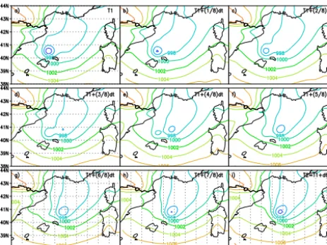
Linear interpolation in time distorts the model fields. Fig-ure 2 shows the effect of linear interpolation on the mean sea level pressure. The ARPEGE forecast mean sea level pres-sure from two consecutive coupling files is interpolated lin-early in time (as in the operational coupling procedure). In the place of a moving storm, LAM sees a dual cyclone struc-ture: one cyclone/storm disappears and another appears. This is why a larger coupling zone yields a dual cyclone structure, as was shown by Tudor and Termonia (2010).
Other meteorological fields that are used for coupling at lateral boundaries get distorted by linear interpolation in time if they contain high-resolution features such as storms or me-teorological fronts. For simplicity, this article will focus on the mean sea level pressure and surface pressure fields.
3 Filtered surface pressure field from ARPEGE 3.1 The time series of MCUF maxima
Figure 2. Mean sea level pressure (hPa) from ARPEGE operational coupling files starting from 12 UTC analysis
on 27thOct 2008, 57 (a) and 60 (i) hour forecasts, linear interpolation of mslp in time to half of the 3 hour
coupling period (e), 1/8 of 3h (b), 1/4 (c) 3/8 (d), 5/8 (f), 3/4 (g) and 7/8 (h).
Table 1. Model, period, horizontal resolution and total number of the coupling files for which the rapid changes
of surface pressure field were analyzed, the field was used received from Meteo-France and computed by
AL-ADIN for files received from ECMWF. The rapid changes in surface pressure for the first 3 hours were ommited
from the analysis due to evidence of model spin-up for some periods.
model period resolution total num whole domain MCUF MCUF>0.003
(from-to) (km) of files >0.003 >0.004 >0.005 coupling zone
ARPEGE 06Z23Jan2006 – 00Z06Feb2008 20.678 64292 906 270 93 235
ARPEGE 06Z06Feb2008 – 00Z11May2010 15.400 72600 1017 383 141 400
ARPEGE 06Z11May2010 – 00Z16Nov2014 10.610 151756 1122 293 125 243
ARPEGE 06Z23Jan2006 – 00Z16Nov2014 all 288648 3045 946 359 878
ARPEGE 06Z01Nov2010 – 00Z16Nov2014 10.610 129674 995 259 108 186
IFS 06Z01Nov2010 – 00Z16Nov2014 15.400 147350 698 178 67 109
23
Figure 2. Mean sea level pressure (hPa) from ARPEGE operational
coupling files starting from the 12:00 UTC analysis on 27 Octo-ber 2008, (a) 57 h and (i) 60 h forecasts, linear interpolation of mean sea level pressure in time to half of the 3 h coupling period (e), 1/8 of 3 h (b), 1/4 (c) 3/8 (d), 5/8 (f), 3/4 (g) and 7/8 (h).
especially in the period until 6 February 2008. Most of the points with large MCUF values in the 3 h ARPEGE forecast are close to mountains. This suggests large spin-up of the surface pressure field in the beginning of the ARPEGE fore-cast. Since these large values of MCUF in the+3 h forecast mostly do not represent a storm that moves quickly through the domain, analysis has been performed only on fields from
+6 h forecast or larger.
MCUF exceeds the 0.003 value rather often, mostly in events that last a few days, up to a week. For each file where MCUF was larger than this threshold value, a figure was plotted with mean sea level pressure from the coupling file (ARPEGE) and the operational ALADIN forecast in 8 km resolution coupled to it, and the points where MCUF was larger than 0.003 (see the example in Fig. 1). Each time, large MCUF values were associated with a pressure disturbance in ARPEGE that was often less intensive in the ALADIN fore-cast (if covered by the operational ALADIN domain).
The events that yield large values of the MCUF field rep-resent RMPDs that rapidly traverse any part of the LACE domain. These events are more frequent in autumn, but ap-pear throughout the year, least often during summer months. Several large MCUF values can be associated with a single event (one cyclone moving rapidly over the model domain), but they represent maxima from different forecast coupling files and different forecast runs (starting from different ini-tial times corresponding to different ARPEGE analyses). On the whole LACE domain, the critical value of 0.003 has been exceeded 3045 times in 288 648 files, more than 1 % of the files in the whole period from 23 January 2006 until 16 November 2014 (see Table 1). In 878 files, large MCUF values were close to the coupling zone of the operational
AL-Figure 3. Maximum value of the MCUF field (units hPa) on
the LACE coupling domain, provided from ARPEGE, from the coupling files for 6 h forecast up to 72 h forecast (60 h for the 18:00 UTC run), starting from the 00:00, 06:00, 12:00 and 18:00 UTC analyses, from 23 January 2006 until 15 Novem-ber 2014.
ADIN domain in DHMZ (see Fig. 1). This is only 0.3 % of the coupling files and the event can be considered rare. But, as mentioned earlier, these events are perhaps most important to be forecast. In order to properly forecast such events us-ing LAM, one should first detect it and then apply boundary error restarts (Termonia et al., 2009) or grid-point nudging (Termonia et al., 2011).
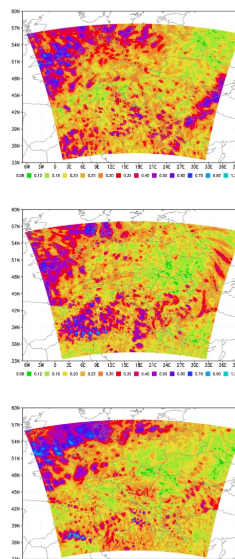
Figure 4. Average MCUF field (unit 0.001 hPa) from ARPEGE
for different resolutions of the LACE coupling files: (a) 20.678 km averaged for the period 23 January 2006 to 6 February 2008.
(b) 15.4 km averaged for the period 6 February 2008 to
11 May 2010. (c) 10.51 km averaged for the period 11 May 2010 to 15 November 2014.
10.51 km) show that it does not depend on the resolution of the coupling files as well as the resolution of the global model where it was computed. The averaged MCUF field is slightly larger over the North Sea in the first period (from 23 Jan-uary 2006 until 6 FebrJan-uary 2008) for the lowest resolution. The values over the Mediterranean have the highest values in the middle period (from 6 February 2008 until 11 May 2010) for the 15.4 km resolution of the coupling files. This result suggests that the cyclones traversed the Mediterranean more often and faster during that period than in the periods before and after.
The maps of the number of cases when the MCUF field exceeded the 0.003 threshold (Fig. 5) show that the number of cases with fast cyclones over the North Sea is the largest in the last period (that is also twice as long as the other two). But over the Mediterranean, MCUF exceeded the critical value most often in the second period, as well as over the area under the influence of the Bay of Biscay.
The absolute maximum values of the MCUF field have large values over most of the western Mediterranean dur-ing the second period (Fig. 6). The overall largest values of MCUF were computed during the third period (and in the highest spatial resolution) close to the coastline of Algeria, but the values are low over the rest of the Mediterranean. On the other hand, the maxima are the highest over the North Sea in the last period and over the Black Sea in the first period.
The spatial distribution of the frequency of the events when MCUF exceeded the critical value (Fig. 5) indicates which areas should be avoided as parts of the coupling zone if one wants to have fewer problems with properly resolv-ing the boundary data in time with a 3-hourly couplresolv-ing up-date period. When the filtered surface pressure field is larger than a threshold value 0.003, there is a storm rapidly prop-agating through the area. If the point with the large value is inside the coupling zone of a LAM, it can be expected that the LAM forecast will miss the storm due to time interpola-tion of boundary data. The analysis of the MCUF field from ARPEGE coupling files for the common LACE coupling do-main shows that this field is above the threshold far more frequently than is acceptable.
4 Detecting rapidly moving pressure disturbances (RMPDs) in the ECMWF coupling files
MCUF is not computed by operational IFS; the alternative methods of detecting RMPDs have been tested on the cou-pling files received operationally from ECMWF.
4.1 Computing MCUF by running the ALADIN model on the coupling files from IFS
Figure 5. The number of times the MCUF field from ARPEGE
exceeds the 0.003 threshold for different resolutions of the cou-pling files: (a) 20.678 km averaged for the period 23 January 2006 to 6 February 2008. (b) 15.4 km averaged for the period 6 Febru-ary 2008 to 11 May 2010. (c) 10.51 km averaged for the period 11 May 2010 to 15 November 2014.
Figure 6. Absolute maximum values of the MCUF field (units
Figure 7. Time series of the maximum value of the IFSM field
(units hPa) on the coupling LACE domain for 6 h forecast up to 78 h forecast, computed by running ALADIN, starting from the 00:00, 06:00, 12:00 and 18:00 UTC analyses from 1 November 2010 until 15 November 2014.
day up to a 78 h forecast with 3-hourly output. The MCUF field computed this way is referred to as IFSM. The initial IFSM values are zero. IFSM computed during the first 3 h of forecast has very large values due to model spin-up, so only the fields corresponding to the 6 h forecast and longer are used in the analysis.
4.1.1 The time series of IFSM maxima
The time series of the maximum values of the IFSM field from the whole LACE domain for forecast ranges from 6 to 78 h are shown in Fig. 7 for the period from 27 October 2010 until 15 November 2014. The critical value is exceeded in 698 files (out of total 147 350 files) during the 4-year period and over the whole domain (see Table 1). This is less often than in ARPEGE, since during the same period MCUF was larger than 0.003 in 995 files (out of 129 674 files). The to-tal number of files is larger for IFS than for ARPEGE since ARPEGE forecast LBC files extend up to 72 h (and only 60 h for the 18:00 UTC run), while files from all runs of IFS ex-tend up to a 78 h forecast.
Although the critical value of 0.003 is exceeded less often with IFSM than with MCUF in ARPEGE, there are periods with large values associated with RMPDs during every part of the year, more often in autumn and the least often in sum-mer. A figure with mean sea level pressure from the IFS cou-pling file and grid points with large IFSM values were plotted for each coupling file for which IFSM exceeded the critical value in order to estimate whether the large IFSM values are associated with the cyclones in the IFS files (and not only in
the ALADIN forecast run used to compute the IFSM field). Inspection of this set of figures led to a conclusion that large values of IFSM are connected to a pressure low in IFS fields. One should keep in mind that the MCUF values are com-puted by running ALADIN using IFS coupling files (ini-tial and forecast). The ALADIN model can yield different evolutions of model variables, including surface pressure, so that large MCUF values correspond to a cyclone that moves quickly in the ALADIN forecast, not necessarily in the IFS forecast. On the other hand, a RMPD in the IFS forecast might be less intensive or slower in the ALADIN forecast due to differences in the model set-up, choices in physics and dynamics.
4.1.2 Spatial distribution of IFSM
MCUF was computed by running ALADIN forecast on a limited area domain in 15.4 km resolution. The coupling zone was eight points wide. The procedure could have missed a cyclone entering the LACE domain during the coupling in-terval. It is also expected to get unwanted phenomena in the IFSM field in the coupling zone of LBC files.
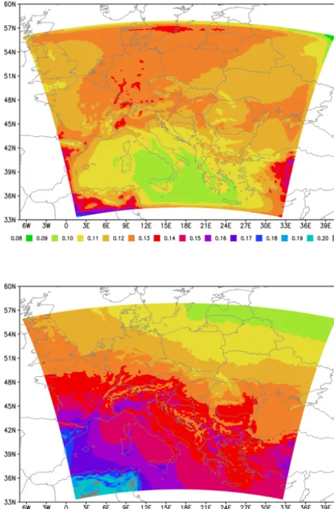
In Fig. 8, a small dot is plotted in the position of each model grid point in the colour corresponding to the aver-age IFSM value multiplied by 1000 as shown in the colour scale below. Average IFSM field and average MCUF from ARPEGE for the same period (Fig. 8) have substantially different spatial distributions. The differences are most pro-nounced over the Baltic area, where IFS yields more fast cy-clones, and over the Mediterranean, where ARPEGE fore-casts more RMPDs.
Figure 8. Spatial distribution of the average IFSM (top) and MCUF
(bottom) values (units 0.001 hPa) for forecast hour greater than or equal to 6 h for the period from 1 November 2010 until 15 Novem-ber 2014.
4.1.3 Computing MCUF by running the ALADIN model on the coupling files from ARPEGE ARPM was computed by running ALADIN on the domain and at the resolution (10.61 km) of the ARPEGE coupling files with a 450 s time step starting from the ARPEGE analy-sis without initialization. The time series of ARPM maxima over the LBC domain are shown in Fig. 11. There is a good agreement with MCUF computed in ARPEGE. But ARPM gives additional a strong signal for the storm that hit Turkey on 27 September 2014. MCUF did not show a signal for the same case.
4.2 The error function values using mean sea level pressure from ECMWF coupling files
ALADIN was run for one time step using fields from the cou-pling files from IFS as initial conditions in order to estimate
Figure 9. Spatial distribution of the maximum of absolute IFSM
(top) and MCUF (bottom) (units 0.01 hPa), for forecast hour greater than or equal to 6 h for the period from 1 November 2010 until 15 November 2014.
the tendency of the model variables (in particular the surface pressure). The run is performed on the grid of the coupling files using a 600 s time step. The error is estimated according to Eq. (1) and its maximum over the model domain according to Eq. (2). The error function was computed for the period from 27 October 2010 until 15 November 2014 for experi-ments without initialization and initialized with SSDFI, and for the period from 1 January 2013 for the experiment with DFI.
4.2.1 Tendencies computed without filtering initialization
Figure 10. Spatial distribution of the number of occurences when IFSM (top) and MCUF (bottom) values
exceed the value 0.003, for forecast hour greater than or equal to 06 hours for the period since 1stNov 2010
until 15thNov 2014.
31
Figure 10. Spatial distribution of the number of occurrences when
IFSM (top) and MCUF (bottom) values exceed the value 0.003, for a forecast hour greater than or equal to 6 h for the period from 1 November 2010 until 15 November 2014.
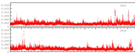
for surface pressure. Due to the rather high level of noise, a critical value larger than 0.003 should be defined in or-der to avoid false alarms. The method using error estimates sometimes yields large values over mountainous areas. If the model domain is defined so that the mountains are not in the intermediate zone (close to lateral boundaries), these events could be ignored by the operational procedure and would not be false alarms.
4.2.2 Tendencies computed with digital filter initialization
The time series of ET computed for fields initialized with DFI is plotted in Fig. 13 for the period from 1 January 2013 until December 2014. The noise is much lower than for the test without initialization, but the signal of RMPDs is also weaker. There is more noise in ET computed for mean sea level pressure than for surface pressure in winter and spring,
Figure 11. Time series of the maximum value of ARPM (MCUF
computed by running ALADIN on the coupling LACE domain from ARPEGE (the domain and resolution of LBC files) with a 450 s time step).
but less in the autumn. The signal of the RMPDs is removed almost completely from the error function computed for sur-face pressure, especially in winter and spring.
There is a signal for RMPD inET computed from mean sea level pressure on 27 November 2013 that does not exist in the time series ofET for the surface pressure. The peak is located over the Alps and shows persistently for model runs from successive analyses about the same time (09:00 to 15:00 UTC that day). The satellite figures of the area for that date show clouds associated with mountain waves (not shown).
4.2.3 Tendencies computed with scale-selective digital filter initialization
Similarly, the error function was computed after the fields in the coupling files have been initialized using SSDFI for the period from 27 October 2010 until December 2014. The time series of the maxima of the error function is plotted in Fig. 14. The level of noise and the intensity of the signal of approaching RMPDs are similar to those computed with DFI. But there are subtle differences. Several cases of RMPDs are more pronounced and there is no signal on 27 Novem-ber 2013 that occurred when DFI was used.
4.3 Amplitude of oscillations in mean sea level pressure The amplitude of oscillations in mean sea level pressure was computed for the coupling files from IFS for the period from 27 October 2010 and for the coupling files from ARPEGE from 1 January 2013, both until December 2014. The time series of the maxima in the amplitude of the mean sea level pressure variations from IFS is displayed in Fig. 15 and for ARPEGE in Fig. 16.
Although the amplitude maxima achieve large values dur-ing periods without RMPDs (the periods without RMPDs are those when MCUF and IFSM are low), the amplitude is so much larger in a case with RMPD that there is a signal that can be distinguished in the noisy pattern.
Figure 12. Time series of the maximum value of the error function
(ET, Eq. 2) without any filtering initialization.
Figure 13. Time series of the maximum value of the error function;
fields are initialized with DFI.
(A >0.003) for each case when this threshold was exceeded. The majority of the cases are related to propagating cyclones and pressure troughs and are usually associated with the large values of IFSM. However, there are cases whenAis larger than the threshold in mountainous regions of the Alps, the Atlas mountains and Turkey, but these are associated with an atmospheric front approaching the area, so the large values could not be dismissed as false.
There are also a number of cases when IFSM did not indi-cate a RMPD, whileAdid reach values above the threshold in points close to the edge of the coupling domain. The subse-quent coupling times also had large values ofAin the vicin-ity. In these cases, the cyclone entered the coupling domain too quickly to be detected by the procedure used to compute the IFSM field.
Figure 14. Time series of the maximum value of the error function;
fields are initialized with SSDFI.
Figure 15. Time series of the maximum value of the amplitude in
the mean sea level pressure variations (Eq. 3) computed from the coupling files from IFS.
5 Conclusions
recom-Figure 16. Time series of the maximum value of the amplitude in
the mean sea level pressure variations (Eq. 3) computed from the coupling files from ARPEGE.
mends choosing carefully the resolution and frequency of large-scale LBCs. However, meteorological services that de-pend on LBCs from elsewhere might have little choice. A coupling update frequency is sufficient if the large-scale model data contain only features that are large enough and slow enough to be resolved by the coupling update period (Denis et al., 2003). Therefore, the coupling update fre-quency is determined by the properties of the global model, not the LAM that uses it for LBCs.
Termonia (2004) developed a strategy to monitor rapid changes in surface pressure in ARPEGE by producing a diag-nostic output field for the filtered surface pressure (MCUF). This field is provided in the coupling files from 06:00 UTC run on 23 January 2006 for the LACE coupling domain.
When MCUF is larger than a threshold value of 0.003 (Ter-monia, 2004), there is a rapid development in the surface pressure, suggesting that a fast cyclone has moved through the area. If the point with the large value is inside the cou-pling zone of the ALADIN domain, it can be expected that the ALADIN model run will miss the cyclone strength and development due to time interpolation of boundary data. When the time series of MCUF data was analysed for the Belgian domain (Termonia et al., 2009), it was found that such events occurred only several times per year.
The analysis of the MCUF field in this article shows that this field is above the threshold more frequently for the whole LACE coupling domain as well as for the coupling zone of the Croatian operational domain (it covers a larger area than the operational Belgian domain in Termonia, 2003), but the event can still be considered rare. There are changes from one season to another (more or less “stormy”), but there is no apparent increase in the number of fast propagating storms, with an increase in the ARPEGE resolution (at least in the range of resolutions available for this study).
The spatial distribution of MCUF reveals that RMPDs favour the sea surfaces, especially the North Sea and the western Mediterranean. Analysis of the MCUF and IFSM fields for a longer period can show which areas favour quickly moving storms that could be missed by the coupling procedure if the 3-hourly coupling period is used. Maps with a number of occurrences when the filtered pressure field is
larger than the 0.003 threshold show that there are not too many places where to put the coupling zone in order to avoid LAM forecast failure in the case of a RMPD. The problem would be only made worse in higher-resolution LAM. The coupling zone on the lateral boundaries is eight grid points wide and shrinks with the resolution increase. The storm needs less time to cross the narrow coupling zone. A higher-resolution global model can yield more intensive pressure changes.
The spatial distribution can be viewed as a map of the fast cyclone tracks and areas that support rapid changes in cy-clone development. Not surprisingly, this study shows that not only North Sea but also the western Mediterranean is an area where storms frequently propagate with high velocities and can not be resolved in LBCs of a 8 km resolution LAM when provided with a 3 h interval. In an LAM with roughly 3 times higher horizontal resolution, even a 1 h coupling in-terval would be insufficient.
There is no field similar to MCUF provided in the coupling files of IFS from ECMWF. Therefore an experiment has been performed in order to compute the field locally from the cou-pling files. The forecast needed to compute MCUF was run using the ALADIN model and the resulting field IFSM can be used for detecting RMPDs in the operational forecast. It requires running the ALADIN forecast in low resolution up to 78 h (same range at which the coupling files are provided). It is more computationally expensive than reading the field already provided in the LBC files, but it is feasible. However, the results contain some detrimental effects:
– different model dynamics could lead to different devel-opments in the surface pressure field and hence different MCUF values,
– a quickly moving storm can enter the LBC domain un-detected and consequently be missed by the MCUF, and – rather low cyclone activity in the western Mediterranean
compared with results using ARPEGE.
The error function (Termonia, 2003) was computed using tendencies estimated by running ALADIN for one time step, using fields from the coupling fields without initialization, initialized with DFI and with SSDFI. No initialization yields a signal of RMPDs, but also a lot of noise. Clearly a higher threshold value should be used, but it should be chosen care-fully. DFI reduces the level of noise and the magnitude of the signal, and many RMPDs are removed from the time series (Fig. 13), but there is still evidence of large values related to mountains. SSDFI reduces the level of noise and the signal of RMPDs, but more of the signal is preserved.
but so is the signal for RMPDs. This method can be used on any variable and it does not require running any model using coupling data as initial conditions. Mean sea level pressure is less sensitive to the reduction in the coupling update fre-quency than precipitation and vorticity (Denis et al., 2003).
Climate LAMs could benefit from a large domain (Žagar et al., 2013). It takes several days for the cascade of variance to fill the small scales (Laprise et al., 2008). Losing small-scale features, arriving from the global model at lateral boundaries, certainly does not help. If the domain of the climate LAM is small and the flow over the area is strong, it could move over the domain too quickly to develop small scales (Žagar et al., 2013), and if the temporal interpolation of LBC data filters high-resolution data from a global model, there might not be enough space (in the domain) or time (before the flow leaves it) for LAM to recreate these small scales.
On the other hand, NWP models that have small-scale data in the initial conditions through blending (Brožkova et al., 2001) or the data assimilation cycle (e.g. Staneši´c, 2011) need RMPDs that enter the domain during the model fore-cast. It took ALADIN 66 h to develop a small-scale feature in the 2 km resolution nonhydrostatic run (Tudor and Ivatek-Šahdan, 2010) coupled to an 8 km operational forecast that was run without data assimilation at the time (Ivatek-Šahdan and Tudor, 2004).
As there are plans to increase the resolution of the op-erational ALADIN to 4 km and ECMWF announced plans for the increase in the horizontal resolution of operational IFS, the problem of resolving RMPDs in LBC data available with a 3-hourly interval will become more frequent and it is questionable whether hourly coupling data would be suffi-cient in some cases. Boundary error restarts (Termonia et al., 2009), grid-point nudging (Termonia et al., 2011), comput-ing corrected interpolation in time with time derivatives (Ter-monia, 2003) and alternative methods of interpolating LBC data in time (Tudor and Termonia, 2010) are computation-ally expensive and should be used only when needed. There-fore such cases should be detected by a reliable method since any missed case means that LAM would not forecast severe weather conditions. The error function computed without ini-tialization and the amplitude method (Sect. 4.3) are cheap methods that could be applied in a straightforward manner. MCUF from IFSM seems reliable for most of the LACE do-main. The error function computed from the initialized fields does not improve the results enough to justify the extra com-putational cost. The alternative is to compute MCUF in op-erational IFS.
Acknowledgements. The author is grateful to the two anonymous reviewers whose constructive comments have improved the manuscript.
Edited by: O. Boucher
References
ALADIN International Team: The ALADIN project: Mesoscale modelling seen as a basic tool for weather forecasting and at-mospheric research, WMO Bull., 46, 317–324, 1997.
Alpert, P., Neeman, B. U., and Shay-El, Y.: Intermonthly variability of cyclone tracks in the Mediterranean, J. Climate, 3, 1474–1478, 1990.
Boyd, J. P.: Limited-Area Fourier Spectral Models and Data Anal-ysis Schemes: Windows, Fourier Extension, Davies Relaxation, and All That, Mon. Weather Rev., 133, 2030–2042, 2005. Brankovi´c, ˇC., Matjaˇci´c, B., Ivatek-Šahdan, S., and Buizza, R.:
Dy-namical downscaling of ECMWF EPS forecasts applied to cases of severe weather in Croatia, ECMWF RD Technical Memoran-dum, No. 507, 38 pp., 2007.
Brankovi´c, ˇC., Matjaˇci´c, B., Ivatek-Šahdan, S., and Buizza, R.: Downscaling of ECMWF Ensemble Forecasts for Cases of Se-vere Weather: Ensemble Statistics and Cluster Analysis, Mon. Weather Rev., 136, 3323–3342, 2008.
Brožkova, R., Klari´c, D., Ivatek-Šahdan, S., Geleyn, J.-F., Casse, V., Široká, M., Rádnoti, G., Janoušek, M., Stadlbacher, K., and Seidl, H.: DFI Blending, an alternative tool for preparation of the initial conditions for LAM, PWRP Report Series No. 31, WMO-TD, No. 1064, 2001.
Campinis, J., Genoves, A., Jansa, A., Guijarro, J. A., and Ramis, C.: A catalogue and a classification of surface cyclones for the Western Mediterranean, Int. J. Climatol., 20, 969–984, 2000. Cassou, C. and Terray, L.: Oceanic forcing of the wintertime
low-frequency atmospheric variability in the north atlantic european sector: a study with the arpege model, J. Climate, 14, 4266–4291, doi:10.1175/1520-0442(2001)014<4266:OFOTWL>2.0.CO;2, 2001.
Courtier, P. and Geleyn, J.-F.: A global numerical weather predic-tion model with variable resolupredic-tion: applicapredic-tion to the shallow water equations, Q. J. Roy. Meteor. Soc., 114, 1321–1246, 1988. Davies, H. C.: A lateral boundary formulation for multi-level pre-diction models, Q. J. Roy. Meteorol. Soc., 102, 405–418, 1976. Davies, H. C.: Limitations of some common lateral boundary
schemes used in regional NWP models, Mon. Weather Rev., 111, 1002–1012, 1983.
Davies, T.: Lateral boundary conditions for limited area models, Q. J. Roy. Meteorol. Soc., 140, 185–196, 2014.
Dee, D. P., Uppala, S. M., Simmons, A. J., Berrisford, P., Poli, P., Kobayashi, S., Andrae, U., Balmaseda, M. A., Balsamo, G., Bauer, P., Bechtold, P., Beljaars, A. C. M., van de Berg, L., Bid-lot, J., Bormann, N., Delsol, C., Dragani, R., Fuentes, M., Geer, A. J., Haimberger, L., Healy, S. B., Hersbach, H., Hólm, E. V., Isaksen, L., Kàllberg, P., Köhler, M., Matricardi, M., McNally, A. P., Monge-Sanz, B. M., Morcrette, J.-J., Park, B.-K., Peubey, C., de Rosnay, P., Tavolato, C., Thépaut, J.-N., and Vitart, F.: The ERA-Interim reanalysis: configuration and performance of the data assimilation system, Q. J. Roy. Meteorol. Soc., 137, 553– 597, doi:10.1002/qj.828, 2011.
Denis, B., Laprise, R., Caya, D., and Cté, J.: Downscaling ability of one-way nested regional climate models: the big-brother experi-ment, Clim. Dynam., 18, 627–646, 2002.
Denis, B., Laprise, R., and Caya, D.: Sensitivity of a regional cli-mate model to the resolution of the lateral boundary conditions, Clim. Dynam., 20, 107–126, 2003.
De Troch, R., Hamdi, R., Van de Vyver, H., Geleyn, J.-F., and Ter-monia, P.: Multiscale Performance of the ALARO-0 Model for Simulating Extreme Summer Precipitation Climatology in Bel-gium, J. Climate, 26, 8895–8915, 2013.
Doswell, C. A., Brooks, H. E., and Maddox, R. A.: Flash flood fore-casting: An ingredients-based methodology, Weather Forecast., 11, 560–581, 1996.
Hamdi, R., Van de Vyver, H., and Termonia, P.: New cloud and mi-crophysics parameterisation for use in high-resolution dynamical downscaling: application for summer extreme temperature over Belgium, Int. J. Climatol., 32, 2051–2065, doi:10.1002/joc.2409, 2012.
Hamdi, R., Van de Vyver, H., De Troch, R., and Termonia, P.: As-sessment of three dynamical urban climate downscaling meth-ods: Brussels’s future urban heat island under an A1B emission scenario, Int. J. Climatol., 34, 978–999, doi:10.1002/joc.3734, 2014.
Haugen, J. and Machenhauer, B.: A spectral limited-area formu-lation with time-dependent boundary conditions applied to the shallow-water equations, Mon. Weather Rev., 121, 2618–2630, 1993.
Hortal, M.: The development and testing of a new two-time-level semi-Lagrangian scheme (SETTLS) in the ECMWF forecast model, Q. J. Roy. Meteorol. Soc., 128, 1671–1687, 2002. Horvath, K., Lin, Y.-H., and Ivancan-Picek, B.: Classification of
cyclone tracks over the Apennines and the Adriatic Sea, Mon. Weather Rev., 136, 2210–2227, 2008.
Horvath, K., Ivatek-Šahdan, S., Ivanˇcan-Picek, B., and Grubiši´c, V.: Evolution and structure of two severe cyclonic bora events: con-trast between the northern and southern Adriatic, Weather Fore-cast., 24, 946–964, 2009.
Horvath, K., Baji´c, A., and Ivatek-Šahdan, S.: Dynamical downscal-ing of wind speed in complex terrain prone to bora-type flows, J. Appl. Meteorol. Climatol., 50, 1676–1691, 2011.
Ivatek-Šahdan, S. and Ivanˇcan-Picek, B.: Effects of different ini-tial and boundary conditions in ALADIN/HR simulations during MAP IOPs, Meteorol. Z., 15, 187–197, 2006.
Ivatek-Šahdan, S. and Tudor, M.: Use of high-resolution dynami-cal adaptation in operational suite and research impact studies, Meteorol. Z., 13, 1–10, 2004.
Laprise, R.: Resolved scales and nonlinear interactions in limited-area models, J. Atmos. Sci., 60, 768–779, 2003.
Laprise, R., de Elía, R., Caya, D., Biner, S., Lucas-Picher, P., Dia-conescu, E., Leduc, M., Alexandru, A., and Separovic, L.: Cana-dian Network for Regional Climate Modelling and Diagnostics: Challenging some tenets of regional climate modelling, Meteo-rol. Atmos. Phys., 100, 3–22, 2008.
Lionello, P., Bhend, J., Buzzi, A., Della-Marta, P. M., Krichak, S. O., Jansá, A., Maheras, P., Sanna, A., Trigo, I. F., and Trigo, R.: Cyclones in the Mediterranean region: climatology and effects on the environment, in: Mediterranean Climate Variability, edited by: Lionello, P., Malanotte-Rizzoli, P., and Boscolo, R., 325–372, Elsevier, 2006.
Lynch, P.: The Dolph–Chebyshev Window: A Simple Optimal Fil-ter, Mon. Weather Rev., 125, 655–660, 1997.
Lynch, P. and Huang, X.-Y.: Initialization of the HIRLAM model using a digital filter, Mon. Weather Rev., 120, 1019–1034, 1992. Lynch, P., Giard, D., and Ivanovici, V.: Improving the Efficiency of a Digital Filtering Scheme for Diabatic Initialization, Mon. Weather Rev., 125, 1976–1982, 1997.
Nicolis, C.: Dynamics of model error: The role of the boundary conditions, J. Atmos. Sci., 64, 204–215, 2007.
Nutter, P., Stensrud, D., and Xue, M.: Effects of coarsely resolved and temporally interpolated lateral boundary conditions on the dispersion of limited-area ensemble forecasts, Mon. Weather Rev., 132, 2358–2377, 2004.
Rádnoti, G.: Comments on A spectral limited-area formulation with time-dependent boundary conditions applied to the shallow-water equations, Mon. Weather Rev., 123, 3122–3123, 1995. Simmons, A. J. and Burridge, D. M.: An Energy and
Angular-Momentum Conserving Vertical Finite-Difference Scheme and Hybrid Vertical Coordinates, Mon. Weather Rev., 109, 758–766, 1981.
Staneši´c, A.: Assimilation system at DHMZ: development and first verification results, Cro. Met. Jour., 44/45, 3–17, 2011.
Staniforth, A.: Regional modelling: A theoretical discussion, Mete-orol. Atmos. Phys., 63, 15-29, 1997.
Termonia, P.: Monitoring and improving the temporal interpolation of lateral-boundary coupling data for limited area models, Mon. Weather Rev., 131, 2450–2463, 2003.
Termonia, P.: Monitoring of the coupling update frequency of a limited-area model by means of a recursive digital filter, Mon. Weather Rev., 132, 2130–2141, 2004.
Termonia, P.: Scale-selective digital filter initialization, Mon. Weather Rev., 136, 5246–5255, 2008.
Termonia, P., Deckmyn, A., and Hamdi, R.: Study of the lateral boundary condition temporal resolution problem and a proposed solution by means of boundary error restarts, Mon. Weather Rev., 137, 3551–3566, 2009.
Termonia, P., Degrauwe, D., and Hamdi, R.: Improving the Tempo-ral Resolution Problem by Localized Gridpoint Nudging in Re-gional Weather and Climate Models, Mon. Weather Rev., 139, 1292–1304, 2011.
Termonia, P., Voitus, F., Degrauwe, D., Caluwaerts, S., and Hamdi, R.: Application of Boyds Periodization and Relaxation Method in a Spectral Atmospheric Limited-Area Model. Part I: Imple-mentation and Reproducibility Tests, Mon. Weather Rev., 140, 3137–3148, doi:10.1175/MWR-D-12-00033.1, 2012.
Tudor, M. and Ivatek-Šahdan, S.: The case study of bura of 1st and 3rd February 2007, Meteorol. Z., 19, 453–466, 2010.
Tudor, M. and Termonia, P.: Alternative formulations for incor-porating lateral boundary data into limited area models, Mon. Weather Rev., 138, 2867–2882, 2010.
Tudor, M., Ivatek-Šahdan, S., Staneši´c, A., Horvath, K., and Ba-ji´c, A.: Forecasting Weather in Croatia Using ALADIN Nu-merical Weather Prediction Model, in: Climate Change and Re-gional/Local Responses, edited by: Zhang, Y. and Ray, P., In-Tech, Rijeka, 59–88, 2013.
M., Berg, L. V. D., Bidlot, J., Bormann, N., Caires, S., Chevallier, F., Dethof, A., Dragosavac, M., Fisher, M., Fuentes, M., Hage-mann, S., Hólm, E., Hoskins, B. J., Isaksen, L., Janssen, P. A. E. M., Jenne, R., Mcnally, A. P., Mahfouf, J.-F., Morcrette, J.-J., Rayner, N. A., Saunders, R. W., Simon, P., Sterl, A., Trenberth, K. E., Untch, A., Vasiljevic, D., Viterbo, P. and Woollen, J.: The ERA-40 re-analysis, Q. J. Roy. Meteorol. Soc., 131, 2961–3012, doi:10.1256/qj.04.176, 2005.
Vánnitsem, S. and Chome, F.: One-way nested regional climate simulations and domain size, J. Climate, 18, 229–233, 2005. Warner, T., Peterson, R., and Treadon, R.: A tutorial on lateral
boundary conditions as a basic and potentially serious limitation to regional numerical weather prediction, B. Am. Meteorol. Soc., 78, 2599–2617, 1997.
Wernli, H., Dirren, S., Liniger, M. A., and Zillig, M.: Dynamical aspects of the life cycle of the winter storm Lothar (24–26 De-cember 1999), Q. J. Roy. Meteorol. Soc., 128, 405–429, 2002. Žagar, N., Honzak, L., Žabkar, R., Skok, G., Rakovec, J., and