A Novel Permutation-based Hash Mode of Operation FP and the Hash Function SAMOSA

(1)

A shortened version of this paper appears under the same title in the proceedings of Indocrypt 2012 (Steven Galbraith and Mridul Nandi, eds.), LNCS, Springer.

A Novel Permutation-based Hash Mode of Operation

FP

and

The Hash Function

SAMOSA

Souradyuti Paul∗ Ekawat Homsirikamol† Kris Gaj2†

Abstract

The contribution of the paper is two-fold. First, we design a novel permutation-based hash mode of operationFP, and analyze its security. The FP mode is derived by replacing thehard-to-invert primitive of theFWP mode – designed by Nandi and Paul, and presented at Indocrypt 2010 – with an easy-to-invert permutation; since easy-to-invert permutations with good cryptographic properties arenormally easier to design, and are more eﬃcient than the hard-to-invert functions, theFPmode is more suitable in practical applications than theFWPmode.

We show that anyn-bit hash function that uses theFPmode is indiﬀerentiable from a random oracle up to 2n/2 _{queries (up to a constant factor), if the underlying 2}_n_-bit

permutation is free from any structural weaknesses. Based on our further analysis and experiments, we conjecture that theFPmode is resistant to all non-trivial generic attacks with work less than the brute force, mainly due to its large internal state. We compare theFP mode with other permutation-based hash modes, and observe that it displays the so far best security/rate trade-oﬀ.

To put this into perspective, our second contribution is a proposal for a concrete hash function SAMOSA using the new mode and the P-permutations of the SHA-3 finalist Grøstl. Based on our analysis we claim that theSAMOSA family cannot be attacked with work significantly less than the brute force. We also provide hardware implementation (FPGA) results forSAMOSAto compare it with the SHA-3 finalists. In our implementations, SAMOSA family consistently beats Grøstl, Blake and Skein in the throughput to area ratio. With more efficient underlying permutation, it seems possible to design a hash function based on theFPmode that can achieve even higher performances.

Keywords. Hash mode, indiﬀerentiability, permutation, FPGA implementation

∗_{University of Waterloo, Canada, and K. U. Leuven, Belgium,}_{souradyuti.paul@uwaterloo.ca}

(2)

1 Introduction

1.1 Block-cipher-based hash modes

Iterative hash functions are generally built from two components: (1) a basic primitive C with finite domain and range, and (2) an iterative mode of operationH to extend the domain of the hash function; the symbolHC denotes the hash function based on the mode Hwhich invokesC iteratively to compute the hash digest. Therefore, to design an efficient hash function one has to be innovative with both the mode H and the basic primitive C. Merkle-Damgärd mode used with a secure block cipher was the most attractive choice to build a practical hash function; some examples are SHA-family [30], and MD5 [34]. The security of a hash function based on the Merkle-Damgärd mode crucially relies on the fact thatC is collision and preimage resistant. The compression function C achieves these properties when it is constructed using a secure block cipher [9]. However, several security issues changed this popular design paradigm in the last decade. The first concern is that the security of Merkle-Damgärd mode of operation – irrespective of the strength of the primitive C – came under a host of generic attacks; the length-extension attack [13], expandable message attack [22], multi-collision attacks [20] and herding attack [10, 21] are some of them. Several strategies were discovered to thwart the above attacks. Lucks came up with the proposal of making the output of the primitiveC at least twice as large as the hash output [26]; this proposal is outstanding since, apart from rescuing the security of the Merkle-Damgärd mode, it is also simple and easy to implement. Another interesting proposal was HAIFA that includes a counter injected into the compression function C to rule out many of the aforementioned attacks [7]. Using the results of [9], it is easy to see that the Wide pipe and the HAIFA constructions are secure when the underlying primitive is a secure block cipher.

(6)

Table 1: Indiﬀerentiability bounds of permutation-based hash modes, where the hash size is n-bit in each case;π denotes the permutation, or one of many equally sized permutations. FPExt1 _{is a natural variant of} _FP _{with parameters shown in the row. The} _ϵ _{is a small} fraction due to the preimage attack on JH presented in [6]. Msg-blk denotes the message block.

Mode of Msg-blk Sizeof π Rate Indiﬀ. bound # of independent operation (ℓ) (a) (ℓ/a) lower upper permutations

Hamsi [24] n/8 2n 0.07 n/2 n 1

Luﬀa [5] n/3 n 0.33 n/4 n 3

Sponge [4] n 3n 0.33 n n 1

Sponge [4] n 2n 0.5 n/2 n/2 1

JH [29] n 2n 0.5 n/2 n(1−ϵ) 1

Grøstl [17] n 2n 0.5 n/2 n 2

FP n 2n 0.5 n/2 n 1

MD6 [14] 6n 8n 0.75 n n 1

FPExt1 6n 7n 0.85 n/2 n 1

1.2 Permutation-based hash modes

For the reasons described in the previous section, the popularity of permutation-based hash functions has been on the rise since the discovery of weaknesses in the Merkle-Damgärd mode. Sponge [3], Grøstl [17], JH [39], Luffa [11] and the Parazoa family [1] are some of them. We note that 9 out of 14 semi-finalist algorithms – and 3 out of 5 finalist algorithms – of the NIST SHA-3 hash function competition are based on permutations. Also, NIST selected Keccak as the winner of the SHA-3 competition, which is a permutation-based Sponge construction. Other notable example is MD6 [35]. In Table 1.2, we compare generic security and performance (measured in terms of rate) of various well known permutation-based hash modes.

1.3 Our contribution

1.3.1 The FPmode

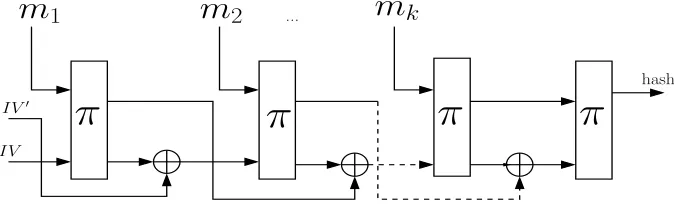
Our ﬁrst contribution is to give a proposal for a new hash mode of operationFPbased on a single wide pipe permutation (see Figure 1). TheFPmode is derived from the FWP(or Fast Wide Pipe) mode designed by Nandi and Paul at Indocrypt 2010 [31].1 The diﬀerence between theFWPand theFPmode is simple: theFPmode is obtained when the underlying

1

(7)

m

k

π

...

m

₁

m

₂

I V′

I V

hash

Figure 1: Diagram of the FP mode. The π is a permutation; all wires are n bits. See Figure 3(a) for the description.

hard-to-invert functionf :{0,1}m+n→ {0,1}2n of the FWP mode is replaced by an easy-to-invert permutationπ :{0,1}2n→ {0,1}2n. There are a number of practical reasons for switching fromFWP toFP: (1) Easy-to-invert permutations are usually efficient, and such permutations with strong cryptographic properties are abundant in the literature (e.g.JH, Grøstl and Keccak permutations); (2) hard-to-invert functions are difficult to design, or they are less efficient.

(8)

1.3.2 Design and FPGA implementation of SAMOSA

Our second contribution is establishing the practical usefulness of the FP mode. As an example, we design a concrete hash function family SAMOSA.2 It is based on the FP mode, where the internal primitives are the P-permutations of the Grøstl hash function. We provide security analysis of SAMOSA, demonstrating its resistance against any known practical attacks.

As demonstrated by the AES and the SHA-3 competitions, the security of a cryp-tographic algorithm alone is not suﬃcient to make it stand out from among multiple candidates competing to become a new American or international standard. Excellent per-formance in software and hardware is necessary to make a cryptographic protocol usable across platforms and commercial products. Assuring good performance in hardware is typ-ically more challenging, since hardware design requires involved and specialized training, and, as it turns out, that the majority of designer groups lack experience and expertise in that area.

In case of SAMOSA, the algorithm design and hardware evaluation have been performed side by side, leading to full understanding of all design decisions and their influence on hardware efficiency. In this paper, we present efficient high-speed architecture ofSAMOSA, and show that this architecture outperforms the best known architecture of Grøstl in terms of the throughput to area ratio by a factor ranging between 24 and 51%. These results have been demonstrated using two representative FPGA families from two major vendors, Xilinx and Altera. As shown in [16], these results are also very likely to carry to any future implementations based on ASICs (Application Specific Integrated Circuits). Additionally, we demonstrate thatSAMOSA consistently ranks above BLAKE, Skein and Grøstl in our FPGA implementations. Although it still loses to Keccak and JH, nevertheless, a relative distance to these algorithms substantially decreases compared to Grøstl, despite using the same underlying operations. This performance gain is accomplished without any known degradation of the security strength.

Additionally, SAMOSA’s dependence on many AES operations makes it suitable for software implementations that use general-purpose processors with AES instruction sets, such as AES-NI. Finally, in both software and hardware,SAMOSA could be an attractive choice for applications where both conﬁdentiality and authentication are required to share AES components. One such example is IPSec, protocol used for establishing Virtual Private Networks, which is one of the fundamental building blocks of secure electronic transactions over the Internet.

Although SAMOSA comes too late for the current SHA-3 competition, it still has a chance to contribute to better understanding of the security and performance bottlenecks of modern hash functions, and to ﬁnd niche platforms and applications in which it may outperform the existing and upcoming standards.

2

(9)

1.4 Notation and convention

Throughout the paper we let n be a ﬁxed integer. While representing a bit-string, we follow the convention of low-bit ﬁrst (or little-endian bit ordering). For concatenation of strings, we usea||b, or justabif the meaning is clear. The symbol⟨n⟩m denotes them-bit encoding of n. The symbol |x| denotes the bit-length of the bit-string x, or sometimes the size of the setx. Let xparse→ x1x2· · ·xk means parsing x intox1,x2,· · ·, xk such that

|x1|=|x2|=· · ·=|xk−1|=nand|xk|=|x|−|x1x2· · ·xk−1|. LetDom(T) ={i|T[i]̸=⊥} andRng(T) ={T[i]|T[i]̸=⊥}. We writeABto denote an AlgorithmAwith oracle access toB. Let [c, d] be the set of integers between c and d inclusive, anda[x, y] the bit-string between thex-th and y-th bit-positions of a. Finally, U[0, N] is the uniform distribution

over the integers between 0 andN. The symbolr←$ A denotes the operation of assigning r with a value sampled uniformly from the setA. The symbol λdenotes the empty string.

2 Deﬁnition of the

FP

Mode

Suppose n ≥ 1. Let π : {0,1}2n → {0,1}2n be the 2n-bit permutation used by the FP mode. The hash function FPπ is a mapping from {0,1}∗ to {0,1}n. The diagram and description of theFPtransform are given in Figures 1 and 3(a), where π is modeled as an ideal permutation. Below we deﬁne the padding functionpad_n(·).

Padding function pad_n(·). It is an injective mapping from {0,1}∗ to ∪i≥1{0,1}ni, where the message M ∈ {0,1}∗ is mapped into a string pad_n(M) = m1· · · mk−1 mk, such that

|mi|=n for 1≤i≤k. The function padn(M) =M||1||0t satisﬁes the above properties (t is the least non-negative integer such that|M|+ 1 +t= 0 modn). Note thatk=

⌈ |M|+1

n ⌉

. In addition to the injectivity of pad_n(·), we will also require that there exists a func-tion dePadn(·) that can eﬃciently compute M, given padn(M). Formally, the function dePadn: ∪i≥1 {0,1}in → {⊥} ∪ {0,1}∗ computes dePadn(padn(M)) = M, for all M ∈

{0,1}∗, and otherwisedePadn(·) returns⊥. The padding rule described above satisﬁes this property also.

3 Indiﬀerentiability Framework: An Overview

We first define the indifferentiability security framework, and briefly discuss its significance.

Definition 3.1 (Indifferentiability framework) [13] An interactive Turing machine (ITM)T with oracle access to an ideal primitiveF is said to be(t_A, t_S, σ, ε)-indifferentiable from an ideal primitive G if there exists a simulator S such that, for any distinguisher A, the following equation is satisfied:

(10)

T F S

A

G

System 1 System 2

(a)

S/S−1

π/π−1

FP1 RO

G0 G1 G2

FP

A A A

≡ _̸≡

S1/S1−1

π/π−1

(b)

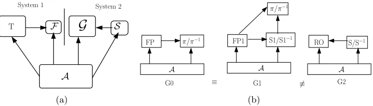
Figure 2: (a) Indifferentiability framework formalized in Definition 3.1; (b) Schematic diagram for the security games used in the indifferentiability framework forFP. The arrows show the directions in which the queries are submitted. System 1 = (T,F) = G0 = (FP, π, π−1), and System 2 = (G,S) = G2 = (RO, S, S−1). See Section 4 for description.

The simulatorS is an ITM which has oracle access toG and runs in time at most t_S. The distinguisher A runs in time at most t_A. The number of queries used by A is at most σ. Hereεis a negligible function in the security parameter ofT. See Figure 2(a) for a pictorial representation. AdvT,_G_,F_S(A) denotes the advantage of adversaryA in distinguishing(T,F) from(G,S).

The signiﬁcance of the framework is as follows. Suppose, an ideal primitive G is indif-ferentiable from an algorithm T based on another ideal primitive F. In such a case, any cryptographic system P based on G is as secure as P based on TF (i.e., G replaces TF in

P). For a more detailed explanation, we refer the reader to [27]. Some limitations of the indifferentiability framework have recently been discovered in [15] and [33]. They offer a deep insight into the framework; nevertheless, the observations arenot known to affect the security of the indifferentiable hash functions in any meaningful way.

An oracle, a system, and a game. An oracle is an algorithm (accessed by another oracle or algorithm) which, given an input as an appropriately deﬁned query, responds with an output. For example, in Figure 2(a), T, F, G and S are oracles. A system is a set of oracles (e.g. System 1 = (T,F), System 2 = (G,S) in Figure 2(a)). A game is the interaction of a system with an adversary. We refrain from providing a formal deﬁnition of a game, since such formalization will not be necessary in our analysis.

4 Main Theorem: Birthday Bound for

FP

Mode

(11)

The description ofFP1,S,S−1,S1, andS1−1 will be provided in Section 10. Now we state our main theorem using Deﬁnition 3.1.

Theorem 4.1 (Main Theorem) The hash function FPπ (or FPπ,π−1) is (t_A, tS, σ, ε )-indiﬀerentiable from RO, where t_A =∞, t_S =O(σ5), and σ ≤K2n/2, where K is a ﬁxed constant derived from ε.

In the next few sections, we will prove Theorem 4.1 by breaking it into several compo-nents. First, we brieﬂy describe what the theorem means: it says that no adversary with unbounded running time can mount anontrivial generic attack on the hash functionFPπ using at mostK2n/2 queries. The parameterK is an increasing function inε, and is con-stant for alln >0. To reduce the notation complexity, we shall derive the indiﬀerentiability bound assumingε= 0.5 for which, we shall derive, K= 1/√56.

Outline of the Proof. Our proof of Theorem 4.1 uses the blueprint developed in [28] and [29] dealing with indiﬀerentiability security analysis of FWP and JH modes of operation. However, to make the paper self-contained, we write out the proof from scratch. The proof consists of the following two components (see Deﬁnition 3.1): (1) Construction of a simulator S = (S,S−1) with the worst-case running time t_S = O(σ5). This is done in Section 10. (2) Showing that, for any adversaryAwith unbounded running time,

Pr[AG0⇒1]−Pr[AG2⇒1]≤ 28σ 2

2n , (1)

where the systems G0 = (FP, π, π−1) and G2 = (RO,S,S−1).The systems G1 and G2 are called the main systems. Proof of (1) is, again, composed of proofs of the following three (in)equations:

• In Sections 8 and 9, we will concretely deﬁne the simulator pair (S,S−1) and a new intermediate system G1. Using them we will show in Section 10,

Pr[AG0⇒1]= Pr[AG1 ⇒1]. (2)

• In Sections 11 and 12, we will appropriately deﬁne a set of eventsBADi andGOODi in the system G1, and will establish that

Pr[AG1⇒1]−Pr[AG2⇒1]≤ σ ∑

i=1

Pr[BADi|GOODi−1

]

. (3)

• In Section 13, we complete proof of (1) by establishing that σ

∑

Pr[BADi |GOODi−1

]

≤ 28σ2

(12)

where

σ ∑

i=1

Pr[BADi |GOODi−1

]

≤ε= 0.5.3

5 Organization of the paper

5.1 Proof of main theorem

Sections 6 to 13 are devoted to complete the proof of Theorem 4.1. The three parts of the proof – i.e., proving (2), (3), and (4) – are done in Sections 10, 12, and 13. These sections make use of the results that are developed in the following sections: Section 6 deﬁnes the data structures used by all systems and proofs; Sections 7, 8, 9, and 11 give detailed description of all the systems.

5.2 Design and implementation of SAMOSA

In Section 14, we propose a new concrete hash function namedSAMOSA, and provide its security analysis. Finally, in Section 15, we give FPGA hardware implementation results forSAMOSA.

6 Data Structures

The systems G0, G1, and G2 have been mentioned in Section 4 (see schematic diagram in Figure 2(b)). The pseudocode of them is given in Figures 3(a), 5, and 3(b). In this section we describe several data structures used by these systems.

6.1 Objects used in pseudocode

6.1.1 Oracles

The main component of a system is the set of oracles that receive queries from the adversary. In Figure 2(b), any algorithm that receives a query is an oracle. Note that, except the adversaryA, each rectangle denotes an oracle.

The systems use a total of 9 oracles. The oraclesFP,FP1, andROare mappings from

{0,1}∗ to {0,1}n. The oracle Sis a mapping from {0,1}2n to{0,1}2n. The permutations π, π−1, S1, and S1−1 are all deﬁned on {0,1}2n, while S−1 is a mapping from {0,1}2n to {0,1}2n ∪ {⊥}. Instruction-by-instruction description of these oracles and the used subroutines are provided in the subsequent sections.

3_Setting 28σ2

2n ≤ε= 1/2, we getσ≤ √1₅₆2n/2. Therefore,K= 1/ √

(13)

6.1.2 Global and local Variables

The oracles described above will use several global and local variables. The local variables are re-initialized every new invocation of the system, while the global data structures main-tain their states across queries. The tablesDl, Ds and Dπ are global variables initialized with ⊥. The graphs Tπ and Ts are also global variables which initially contain only the root node (IV, IV′). Other than them, all other variables are local, and they are initialized with⊥.

6.1.3 Query and round: deﬁnitions

In Figure 2(b), an arrow denotes a query. The submitter and receiver algorithms of a query are denoted by the rectangles attached to the head and the tail of the arrow.

Long query. Any query submitted toFP,FP1, or ROis along query. A long query and its response are stored in the tableDl.

Short query. Queries submitted to S,S1 are s-queries, and those submitted to S−1 and S1−1 as s−1-queries. The s- and s−1-queries and their responses are stored in table Ds. Similarly, queries submitted toπ, andπ−1 are π- andπ−1-queries; these queries and their responses are stored in table Dπ. Each of the above queries is classiﬁed as short query. Note that, for G0,Ds=∅; for G1, Dπ ⊇Ds; and, for G2,Dπ =∅.

Fresh and old queries. Thecurrent short query can also be of two disjoint types: (1) an old query, which is already present in the relevant database (e.g. for G1, when an adver-sary submits an s-query which is an intermediate π-query of a previously submitted long query); or (2) afresh query, which is so far not present in the relevant database.

Message block. In order to compare the time complexities of the oraclesFP,FP1 andRO on a uniform scale, we recall the notion of amessage block. A long query M – irrespective of the oracle – is assumed to be a sequence of k message blocks m1, m2, · · · mk, where pad_n(M) =m1m2· · ·mk. Note that, forFPand FP1, every message blockmi corresponds to a π-queryx||mi for some bit-string x. However, it is not known how the ROprocesses the message blocks of a long query M. We assume that the RO processes the message blocks sequentially, and that the time taken to process a message block is the same for all FP,FP1 and RO.

(14)

Rules of the game. An adversary never re-submits an identical query. Moreover, an s-query (or s−1-query) is also not submitted, if it matches with the output of a previous s−1-query (or s-query).

6.2 Graph theoretic objects used in proof of main theorem

In addition to objects deﬁned in the section above, we will use the following notions for a rigorous mathematical analysis of our results.

Suppose, π:{0,1}2n→ {0,1}2n is an ideal permutation, andD is a ﬁnite set of pairs of the form (x, π(x)).

6.2.1 Reconstructible message

From the high level, M is a reconstructible message for the set D, if D contains all the π-queries and responses (x, π(x)), required to compute FPπ(M).

More formally, M is a reconstructible message for D, if, for all 0 ≤ i ≤ k−1, (yimi+1, π(yimi+1))∈D, where padn(M) =m1m2· · ·mk and yi+1yi′+1=π(yimi+1)⊕(yi′||0).

6.2.2 (Full) Reconstruction graph

To put it loosely, areconstruction graph storesreconstructible messages on its branches. A full reconstruction graphstoresall reconstructible messages. We now deﬁne them formally. A weighted digraphT = (V, E) is deﬁned by the set of nodes V, and the set of weighted edgesE. A weighted edge (v, w, v′)∈E is an ordered triple, such thatv, v′ ∈V, and wis the weight of the ordered pair (v, v′).

Deﬁnition 6.1 (Reconstruction graph) Suppose a weighted digraphT = (V, E)is such thatV is a set of 2n-bit strings, and, for all(a, b, c)∈E, the weight b is an n-bit string.

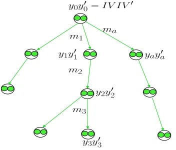
The graph T is called a reconstruction graph for D if, for every(y1y1′, m2, y2y′2)∈E, the following equation holds: y2y′2=π(y1m2)⊕(y′1||0)(all variables arenbits each), where (y1m2, π(y1m2)) ∈ D . (An example of reconstruction graph is given in Figure 4, which will be discussed in detail in the subsequent sections.)

A branchB of a reconstruction graphT, rooted at IV IV′, isfertile, ifdePadn(m1 m2· · · mk)̸=⊥,where{m1, m2,· · ·, mk} is the sequence of weights on the branchB.

Remark: Each fertile branch of a reconstruction graph corresponds to exactly one recon-structible message.

(15)

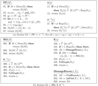
FP(M)

01. If M ∈Dom(Dl)then

returnDl[M];

02. m1m2. . . mk:=padn(M);

03. y0:=IV,y′0:=IV′; 04. for(i:= 1,2, . . . k)

yiy′i:=π(yi−1||mi)⊕(y′i−1||0); 05. r:=π(yk||y′k);

06. Dl[M] :=r[n,2n−1];

07. returnDl[M];

π(x)

11. If x /∈Dom(Dπ)

thenDπ[x]

$

← {0,1}2n\Rng(Dπ);

12. returnDπ[x]; π−1(r)

21. If r /∈Rng(Dπ)

thenD−1

π [r]

$

← {0,1}2n_\_Dom₍_D π);

22. returnD−1

π [r];

(a) System G0 = (FP,π,π−1). For alli,|mi|=|yi|=|y′i|=|r/2|=n.

RO(M)

001. If M ∈Dom(Dl)then

returnDl[M];

002. Dl[M]← {$ 0,1}n;

003. returnD_l[M]; S−1(r)

300. x← {$ 0,1}2n;

301. if x∈Dom(Ds)thenAbort;

302. Ds[x] :=r;

303. FullGraph(Ds);

304. returnx;

S(x)

100. r← {$ 0,1}2n_;

101. if r∈Rng(Ds)thenAbort;

102. M:=MessageRecon(x, Ts);

103. if |M|= 1then

r[n,2n−1] :=RO(M); 104. Ds[x] :=r;

105. FullGraph(Ds);

106. returnr;

MessageRecon(x, Ts)

201. M′:=FindBranch(x, Ts);

202. M:={dePad(X)|X ∈ M′}; 203. returnM;

(b) System G2 = (RO,S,S−1).

Figure 3: The main systems G0 and G2

6.2.3 View

Very loosely, the data structureviewrecords the history of the interaction between a system and an adversary. Letxiandyibe thei-th query from the adversary and the corresponding response from the system. Theviewof the system afterjqueries is the sequence of queries and responses{(x1y1), . . . ,(xjyj)}.

7 Main System G0

(16)

8 Main System G2

See Figure 3(b) for the pseudocode. The random oracle ROdeﬁned in Section 4 is imple-mented through lazy sampling. The only remaining part is to construct the simulator-pair (S,S−1). Our design strategy for the simulator-pair is fairly straightforward and simple. Before going into the details, we ﬁrst provide a high level intuition.

8.1 Intuition for the simulator pair (S,S−1)

The purpose of the simulator pair (S,S−1) is two-pronged: (1) to output values that are indistinguishable from the output from the ideal permutation (π, π−1), and (2) to respond in such a way that FPπ(M) and RO(M) are identically distributed. It will easily follow that as long as the simulator-pair (S,S−1) is able to output values satisfying the above conditions, no adversary can distinguish between G0 and G2.

To achieve (1), the simulator S, for a distinct input x, should output a random value, such that the distributions ofS(x) and π(x) are close. Similarly, the simulator S−1, for a distinct input r, should give outputs such that the random variables S−1(r) and π−1(r) follow statistically close distributions.

To achieve (2), the simulator-pair needs to generate reconstructible messages from the setDs. To accomplish this, it needs to do the following:

•Assessing the power of the adversary: To asses the adversarial power the simulator-pair (S, S−1) maintains the full reconstruction graph Ts for the set Ds that contains all s-, s−1-queries and responses; this helps the simulator keep track of all ‘FP-mode-compatible’ messages (more formally, all reconstructible messages) that can be formed using the el-ements of Ds. This is accomplished by a special subroutine FullGraph. The pictorial representation of the reconstruction graphTs is given in Figure 4.

•Adjusting the elements of the tablesDlandDs: Whenever a new reconstructible message M is found, the simulator makes this crucial adjustment: it assigns FPS(M) := RO(M). It is fairly intuitive that, if S and π produce outputs according to statistically close dis-tributions, then the distributions ofFPS(M) and FPπ(M) are also close. SinceFPS(M) = RO(M), the distributions of RO(M) and FPπ(M) are also close. This is accomplished by the subroutineMessageRecon.

8.2 Detailed description of the simulator pair (S,S−1)

We ﬁrst describe the two most important parts of the simulator-pair: the subroutines Full-Graphand MessageRecon.

(17)

creating all possible nodes, and ﬁnally connecting them to create the graph Ts. In Ap-pendix B, we compute the running time of FullGraph on thei-th query to beO(i4).

MessageRecon(x, Ts). The graph Ts is already the full reconstruction graph for the set Ds. Given the current s-query x, this subroutine derives all newreconstructible messages M, such that, in the computation of FPS(M), the ﬁnal input to S is x, and all other intermediate inputs toSare old s-queries.

To determine such messages M, ﬁrst, FindBranch(x, Ts) collects all branches between the nodes (IV, IV′) and x; then, it selects the sequence of weights X = m1m2· · ·mk for all such branches. Finally it returns a set{M =dePad(X)} for allX. If no suchM ̸=⊥is found, then the subroutine returns the empty set.

m2

y0y0′ =I V I V′

ma

yaya′

y2y′2

m3

y3y3′ m1

y1y1′

Figure 4: The reconstruction graphTs(orTπ) updated byFullGraphof G2 (orPartialGraph of G1).

With the deﬁnition of the above subroutines, we now describe howS and S−1 respond to queries.

An s-query and response (for S): For ans-query, the simulatorS assigns a uniformly sampled 2n-bit value tor; ifrmatches an old range point inDsthen the round is aborted.4 Then the subroutineMessageRecon(x, Ts) is invoked which returns a set of reconstructible messages M. If |M| = 1 then the RO is invoked on M ∈ M, and the value is assigned to r[n,2n−1]. Finally, the graph Ts is updated by FullGraph, before r is returned. In Appendix B, we show that the worst-case running time of Safter σ queries is O(σ5).

An s−1-query and response (for S−1): For an s−1-query, the simulator S−1 assigns a uniformly sampled 2n-bit value to x; if x matches an old domain point in Ds then the

4

(18)

round is aborted. Finally, the graphTs is updated byFullGraph, before x is returned. In Appendix B, we show that the worst-case running time ofS−1 after σ queries isO(σ5).

9 Intermediate system G1

The pseudocode is provided in Figure 5. For the sake of clear understanding, we ﬁrst discuss the motivation for designing this system.

9.1 Motivation for G1

The main motivation for constructing a new system G1 is that it is difficult to compare between the executions of the systems G0 and G2, instruction by instruction. The diffi-culty arises from the fact that G2 has a graph Ts, and two extra subroutines FullGraph, and MessageRecon, while G0 has no such graphs or subroutines. To get around this diffi-culty, we reduce G0 to an equivalent system G1 by endowing it with additional memory for constructing a similar graphTπ, and supplying it with the additional subroutines Mes-sageRecon and PartialGraph. These additional components do not result in any difference in the input and output distributions of the systems G0 and G1 for any adversary (this result is formalized in Proposition 10.1); therefore, in the indifferentiability framework, G0 can be replaced by G1.

Even though G1 and G2 now appear ‘close’, there are still important diﬀerences. The most crucial of them is that, in the former case, the long queries are processed as a sequence of π-queries; therefore, current s- and s−1-queries of G1 may match old π-queries and responses, while such events are not possible for G2. This diﬀerence comes with two implications:

1. The reconstruction graph Tπ in G1 is built using s-, s−1-, π-queries, and their re-sponses stored in the table Dπ; in case of G2, the reconstruction graph Ts is built usingonly s-,s−1-queries and responses stored inDs. This diﬀerence can be identi-ﬁed by separating out, fromTπ, the maximally connected subgraph Ts built from all thes-,s−1-queries and responses stored inDs in G1. Now the reconstruction graph Ts in both systems are comparable.

(19)

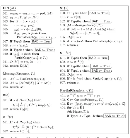
FP1(M)

001. m1m2· · ·mk−1mk:=padn(M); 002. y0:=IV,y′0:=IV′;

003. for(i:= 1,· · ·, k){ 004. r:=π(yi−1mi); 005. yiy′i:=r⊕(y′i−1||0); 006. if yi−1mi is fresh then

PartialGraph(yi−1mi, r, Tπ);} 007. if Type3then BAD:= True ; 008. r:=π(yky′k);

009. if Type0-bthen BAD:= True ; 010. if yky′k isfresh then

PartialGraph(yky′_k, r, Tπ); 011. Dl[M] :=r[n,2n−1]; 012. return Dl[M];

MessageRecon(x, Ts)

201. M′ :=FindBranch(x, Ts); 202. M:={dePad(X)|X∈ M′}; 203. return M;

π(x)

301. if x /∈Dom(Dπ) then

Dπ[x] $

← {0,1}2n\Rng(Dπ); 302. return Dπ[x];

π−1(r)

501. If r /∈Rng(Dπ) then

D_π−1[r]← {$ 0,1}2n\Dom(Dπ); 502. return D_π−1[r];

S1(x)

100. If Type2 then BAD:= True ; 101. r :=π(x);

102. if Type0-athen BAD:= True ; 103. M:=MessageRecon(x, Ts);

104. if |M|= 1∧M /∈Dom(Dl) then Dl[M] :=r[n,2n−1];

105. Ds[x] :=r;

106. if xis fresh thenPartialGraph(x, r, Tπ); 107. returnr;

S1−1(r)

601. if Type4then BAD:= True ; 602. x:=π−1(r);

603. if Type0-cthen BAD:= True ; 604. if Type1-cthen BAD:= True ; 605. Ds[x] :=r;

606. if r isfresh thenPartialGraph(x, r, Tπ); 607. returnx;

PartialGraph(x, r, Tπ)

401. xparse→ ycm;r parse

→ y∗y′; 402. C:=ContactPoints(yc, Tπ);

403. E:={(ycyc′, m, yy′)|y:=y∗⊕y′c, ycy′c ∈C}; 404. for ∀e∈E {

AddEdge(e, Tπ);

if Type1-a∨Type1-bthen BAD:= True ;}

(20)

9.2 Detailed description of G1

Now we describe G1 in detail. For the moment, we postpone the description of the Type0,1, 2, 3 and 4 events until Section 11, since they do not impact the output and the global data structures of G1. We ﬁrst discuss the subroutines used by the oraclesFP1,S1 and S1−1.

PartialGraph(x, r, Tπ). This subroutine is invoked whenever a freshπ- andπ−1-query – with r=π(x) – is encountered. The subroutine updates the reconstruction graphTπ with (x, r) in the following way: First, the subroutineContactPoints(yc =x[0, n−1]) is invoked, that returns a setCcontaining all nodes in Tπ withyc being least signiﬁcantnbits. The size of C determines the number of fresh nodes to be added toTπ in the current iteration. Using the members ofC and the new pair (x, r), new weighted edges are constructed, stored in E, and added to Tπ using the subroutineAddEdge. See Figure 4 for a pictorial description. Note that the reconstruction graphTπ may not be full for the elements inDπ; hence the namePartialGraph.

MessageRecon(x, Ts): This subroutine has been described already in the context of G2, that determines new reconstructible messages. Note that the graph Ts is the maximally connected subgraph of Tπ with the root-node (IV, IV′), generated by the s-, s−1-queries and responses stored inDs;xis the current s-query.

Now we describe how the oraclesS1,S1−1, and FP1 respond to queries.

An s-query and response (for S1): For the s-query x, S1 computes π(x). Then the subroutine MessageRecon(x, Ts) is called which returns a set of reconstructible messages

M. If |M|= 1, and the M ∈ Mis not a previous long query thenDl[M] is assigned the value of π(x)[n,2n−1]. Before ﬁnally returning r, the subroutine PartialGraph is called with input (x, r), if it is fresh, to update the existing graph Tπ.

Ans−1-query and response (for S1−1): For an s−1-queryr,xis assigned the value of π−1(r). Finally,Ds[x] and Tπ are updated, and x is returned.

A long query and response (for FP1): FP1 mimics FP, while updating the graphTπ using the subroutinePartialGraph, whenever afreshπ-query is generated. Dl[M] is assigned r[n,2n−1], wherer is the output from the ﬁnalπ call. Finally, r[n,2n−1] is returned.

10 First Part of Main Theorem: Proof of

(2)

(21)

Proposition 10.1 For any distinguishing adversary A,

Pr[AG0 ⇒1]= Pr[AG1 ⇒1].

Proof. From the description of S1 and S1−1, we observe that, for all x ∈ {0,1}2n,

S1(x) =π(x) and S1−1(x) =π−1(x). Likewise, from the descriptions of FP1 andFP, for

allM ∈ {0,1}∗,FP1(M) =FP(M). 2

11 Type0, 1, 2, 3, and 4 of System G1

In this section, we concretely deﬁne the Type0, Type1, Type2, Type3 and Type4 events of the system G1 (see Figure 5). Informally they will be called ‘bad’ events, since these events set the variableBAD in G1. We ﬁrst provide the motivation for these events.

11.1 Motivation

We recall that the adversary submitss-,s−1- and long queries to the system G1 and receives responses, and based on the history of query-response pairs, known asview– she then tries to distinguish G1 from G2. Intuitively, those events are called ‘bad’, for which the outputs from theπandπ−1 oracles of G1 can be predicted by the adversary with probability better than when interacting with G2. These events primarily involve various forms of collision, occurring in the graph Tπ, allowing the adversary to generate non-trivial reconstructible messages. Secondly, we need to catch the events where current queries match old queries too. One can intuit that these events help the adversary in distinguishing G1 from G2. It is also important to note that, ifTπ is not afull reconstruction graph then the adversary can also use this fact to compel G1 to produce outputs diﬀerent from those from G2 (since G2 always maintains the full reconstruction graphTs).

Next sections deal with concrete deﬁnitions of these events, keeping the above motiva-tion in mind.

11.2 Classifying elements of Dπ, branches of Tπ, and π/π−1-queries

The Type0 to Type4 events depend on the elements in Dπ, the branches of Tπ, and the types of π- andπ−1-queries. In the following sections we ﬁrst classify them.

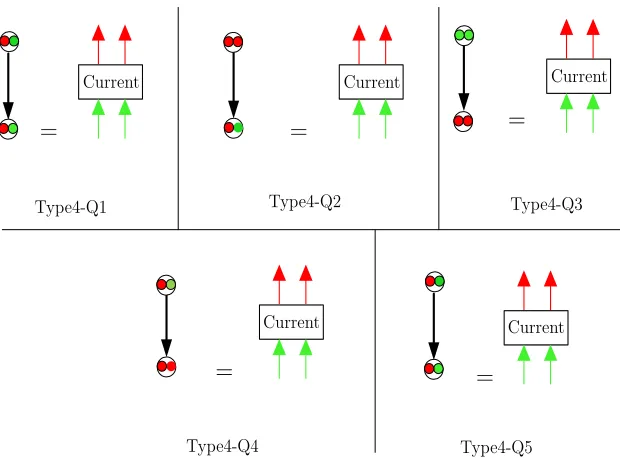
11.2.1 Elements of Dπ: six types

(22)

there are six types of such a pair, and we denote them by Q0, Q1, Q2, Q3, Q4 and Q5 in Figure 6(a); the head and tail nodes – each 2nbits – denote the input to, and the output from the query. Two-sided arrowhead indicates that the corresponding input-output pair is generated from either a π-or a π−1-query. The red and green circles – each n bits – denoteunknown andknown parts.

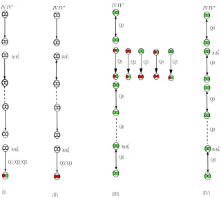
11.2.2 Branches ofTπ: four types

The branches ofTπ can be classified into four types, as shown in Figure 6(b). A branchB is: type I, if the final query is Q1, Q2 or Q5; type II, if the final query is Q3 or Q4; type III, if the final query is Q0, and if one of the intermediate queries is Q1, Q2, Q3, Q4 or Q5; type IV, if all queries are Q0. The first three types are calledred branch. The fourth type is calledgreen branch.

11.2.3 The π- and π−1-queries: nine types

We observe that – based on the types described in the sections above – the currentπ- and π−1-query can be categorized into the following classes.

1. Currentπ-query is ans-query. This can be of two types.

(a) Theπ-query is fresh.

(b) Theπ-query is one of six types of elements inDπ described in Section 11.2.

2. Currentπ−1-query is ans−1-query. This can be of two types.

(a) Theπ−1-query is fresh.

(b) Theπ-query is one of six types of elements inDπ.

3. Current π-query is an intermediate π-query for the current long query. This is of three types.

(a) Current long query is present on ared branch – as deﬁned in Section 11.2 – of the graph Tπ. Theπ-query in this case is necessarily one of six types stored in Dπ; we divide it into two cases.

i. The π-query is the ﬁnal one. ii. The π-query is a non-ﬁnal one.

(b) Current long query is present on agreen branch of the graphTπ. The π-query in this case is also one of six types stored inDπ.

(c) Current long query is not present on a branch of the graph Tπ. We divide the π-query into two types.

i. The π-query is fresh.

(23)

Q0

Q1

_Q2

_Q3

Q4

Q5

(a) Q0, Q1, Q2, Q3, Q4, and Q5 denote six types ofπ/π−1_{-query and} response.

IV IV′

Q1 Q2 Q3 Q4 Q5 Q0

Q0

IV IV′

Q0

IV IV′

Q3/Q4

Q0

IV IV′

Q1/Q2/Q5

(I)

(II) (III) (IV)

y1y′1

yky′k ykyk′

y1y1′

yky′k _y ky′k

y1y1′

(b) Several types of a branch inTπ. (I), (II) and (II) are calledredbranch. (IV)

is calledgreen branch.

(24)

11.3 Type0 and Type1 on Fresh queries

11.3.1 Intuition

We address the classes 1a, 2a, and 3ci of Section 11.2.3 together, since they are connected by the fact that the π- or π−1-query is fresh. It is straightforward to notice that, if the outputs of the fresh queries are uniformly distributed, then distinguishing between G1 and G2 is diﬃcult: Type0 events are designed to measure the degree to which the outputs of theπ- and π−1-queries are uniformly distributed.

The second scenario is when the adversary is able to generate a non-trivial reconstruc-tion message, for distinguishing G1 from G2. This is possible, if the freshπ-query causes a node collision in the graphTπ, or if it causes an old query to be attached to a fresh node, or if ans−1-query can be attached to a node ofTπ. Type1 events cover these events. In ad-dition, we require that the absence of these events make the graphTπ a full reconstruction graph. Detailed descriptions are below.

11.3.2 Type0: Distance from the uniform

Type0 event occurs when the output of a fresh π/π−1-query is distinguishable from the uniform distribution U[0,22n−1]. A Type0 event can be of three types: event Type0-a occurs when a fresh π-query is an s-query; event Type0-b occurs when a fresh π-query is the ﬁnal π-query of a long query; event Type0-c occurs when an s−1_{-query is a fresh} π−1-query.

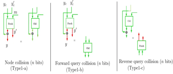
Fresh Old Fresh

Old

= =

Fresh

=

m y_c′ yc

Node collision (nbits) Forward query collision (nbits)

y

y′ y′

yc y′c

y

(Type1-a) _(Type1-b)

Reverse query collision (nbits) (Type1-c)

Old

Figure 7: Type1 events of G1. All arrows are nbits each. Red arrow denotes freshn bits of output from the ideal permutation π/π−1_{. The symbol “=” denotes}_n_{-bit equality.}

11.3.3 Type1: Collision in Tπ

(25)

adversary, (2) the growth ofTπ every round is “small”, and (3)Tπ is afull reconstruction graphfor the set Dπ.

• Type1-a. Suppose yy′ is a fresh 2n-bit node generated when a fresh π-query is attached to Tπ. This event occurs when yy′ collides with another node in Tπ; this collision can be used to generate at least two reconstructible messages in the next rounds – one of them can be used to distinguish G1 from G2. It is important to note that, even though we are interested in 2n-bit node collision, Type1 event captures collision on the least signiﬁcant n bits of the nodes. Therefore, it includes a bigger set of events than necessary. This is done to bound the growth of the graph; more precisely, it allows at most one fresh node to be added in the next round, if this event does not occur.

• Type1-b. Suppose yy′ is a fresh node as defined above. This event occurs if yy′ collides with any element in Dom(Dπ); like before, this event can also be used to form a non-trivial reconstructible message. In a similar manner as Type1-a, we define Type1-b event wheny collides with the least significant nbits of any element inDom(Dπ), and, as a result, it covers more events than required. Exactly like the Type1-a event, this is used to bound the growth of the graph, that is, it ensures that no new nodes can be added toTπ in the present round, if this event does not occur.

• Type1-c. This event occurs when the output of the currents−1-query collides with any node in Tπ, and thereby, the absence of this event precludes the formation of a reconstructible message. Like the previous two types, we deﬁne this event when a node and the output of thes−1 query collide on the least signiﬁcant n bits. The absence of this event ensures that the s−1-query is notadded toTπ.

Remark: Our conservative choice of Type1 events, eventually, degrades the indiﬀerentia-bility bound of FP. The bound of n/2 bits of this paper seems likely to be improved by relaxing the above conditions. We experimented with a smaller set of events than the ones mentioned above, and obtained an indiﬀerentiability bound very close tonbits. However, constructing a theoretical proof of that turns out to be an involving task.

11.4 Type2, Type3 and Type4 on Old queries

11.4.1 Intuition

Now we deal with the classes 1b, 2b, 3a, 3b and 3cii of Section 11.2.3. All of them address the issue when the current queries match old ones.

(26)

The remaining classes are now 3a, 3b and 3cii, when the adversary submits a long query – say M – to the oracle FP1, and it is found that M is already present on some (fertile) branch of the graphTπ (3a and 3b), or it is not presentat allon any branch ofTπ (3c). The class 3c necessarily includes a freshπ-query, and this scenario has already been considered in Type0, and Type1; one can also see that class 1b (or Type2 events) already included the class 3cii. So we skip them here. The other classes – 3a and 3b – are crucial now, and they represent whenM corresponds to an already presentredorgreenbranch of Tπ (deﬁnitions in Section 11.2). We ignore the classes 3b, and 3aii, since they do not help the adversary in distinguishing systems.

So now we focus on the class 3ai, which deals with the final π-query of a red branch. Depending on the type of branch, the adversary tries to predict the most significantnbits of the finalπ-query (i.e.,the hash output) with non-trivial probability; she succeeds only for Type3 events that will be discussed shortly.

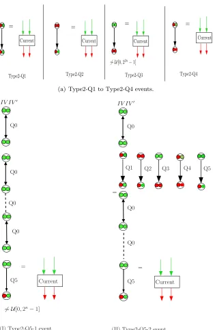
11.4.2 Type2

Recall that a query-response pair in Dπ can be of six types: Q0 to Q5. Type2 event is divided into several cases depending on the type of the current s-query.

Type2-Q1, Type2-Q2, and Type2-Q4events occur, if the s-query is type Q1, Q2 and Q4 respectively.

Type2-Q3 event occurs, if the s-query is type Q3, and if the most signiﬁcant n bits are distinguishable from the uniform distribution.

Type2-Q5. We observe that a Q5 query can be located in two diﬀerent types of branch inTπ, as shown in Figures 8(b)(I) and (II).

• Type2-Q5-1occurs if the current s-query is Q5, and is located in a type I branch, and if the least signiﬁcantnbits are distinguishable from random.

• Type2-Q5-2occurs if the currents-query is Q5, and is located in a type II branch.

11.4.3 Type3

In this case, we consider the ﬁnal π-query of a red branch as the current query. Several types of red branch – (I), (II), and (III) – are shown in Figure 6(b)(I) to (III).

There are three types of Type3 event: (Type3-a) if the current long query M with m1m2· · ·mk=padn(M) forms ared branch of type (I).5 (Type3-b) ifM is ared branch of

5

Observe that this case implies a node collision inTπ, since theyky′kis the finalπ-query for two distinct

(27)

=

Current

Current Current

=

Type2-Q4 Type2-Q3

̸∼ U[0,22n₋_1]

Type2-Q2 Type2-Q1

= =

Current

(a) Type2-Q1 to Type2-Q4 events.

(II) Type2-Q5-2 event

IV IV′

Q1 Q2 Q3 Q4 Q5

IV IV′

=

Current

=

Current =

̸∼ U[0,2n₋_1]

Q0

Q5 _Q5

(I) Type2-Q5-1 event

(b) Type2-Q5 events; they are subdivided into Type2-Q5-1 and Type2-Q5-2. The branches in (I) and (II) represent long queries.

(28)

Current

=

₌

Type4-Q1 Type4-Q2 Type4-Q3

Type4-Q5 Type4-Q4

Current Current Current

Current

Figure 9: Several types of Type4 events: Type4-Q1 to -Q5

type (II), and if the most signiﬁcantnbits of output can be distinguished from the uniform distributionU[0,2n₋_{1]. (Type3-c) if} _M _{is a}_red _{branch of type (III).}

11.4.4 Type4

This event is shown in Figure 9. The Type4 event occurs, if the currents−1-query is equal to the output of an old query of type Q1, Q2, Q3, Q4 or Q5.

12 Second Part of Main Theorem: Proof of

(3)

With the help of the Type0 to Type4 events described in Sections 11.3, and 11.4, we are equipped to prove (3). First, we first fix a few definitions.

12.1 Deﬁnitions: GOODi and BADi

GOODi and BADi. BADi denotes the event when the variable BADis set during round i of G1, that is, when Type0, Type 1, Type2, Type3 or Type4 events occur. Let the symbol GOODi denote the event ¬

∨i

j=1BADi. The symbol GOOD0 denotes the event when no queries are submitted. From a high level, the intuition behind the construction of the

(29)

BADi event is straightforward: we will show that ifBADi does not occur, and ifGOODi−1 did occur, then theviews of G1 and G2 (afterirounds) are identically distributed for any attackerA.

GOOD1i and BAD1i. In order to get around a small technical diﬃculty in establishing the uniform probability distribution of certain random variables, we need to modify the above eventsGOODi andBADi slightly. The eventBAD1i occurs when Type0, Type2, Type3 or Type4 events occur in thei-th round. The eventGOOD1i is deﬁned asGOODi−1∧¬BAD1i.

12.2 Proof of (3)

To prove (3) we need to show two things:

Pr[AG1⇒1]−Pr[AG2⇒1]≤Pr[¬GOOD1σ ]

, (5)

Pr[¬GOOD1σ ]

≤Pr[¬GOODσ ]

≤

σ ∑

i=1

Pr[BADi |GOODi−1

]

. (6)

The proof of (6) is straight-forward. To prove (5), we proceed in the following way. Observe

Pr[AG1 ⇒1]−Pr[AG2 ⇒1]

=

(

Pr[AG1 ⇒1|GOOD1σ ]

−Pr[AG2 ⇒1|GOOD1σ ])

·Pr[GOOD1σ ]

+

(

Pr[AG1⇒1| ¬GOOD1σ ]

−Pr[AG2⇒1| ¬GOOD1σ ])

·Pr[¬GOOD1σ]. (7)

If we can show that

Pr[AG1 ⇒1|GOOD1σ ]

= Pr[AG2 ⇒1|GOOD1σ ]

, (8)

then (7) reduces to (5), since

Pr[AG1 ⇒1| ¬GOOD1σ ]

−Pr[AG2 ⇒1| ¬GOOD1σ]≤1.

As a result, we focus on establishing (8), which is done in Appendix C.

13 Third (or Final) Part of Main Theorem: Proof of

(4)

To prove (4), we need individually compute the probabilities Type0, Type1, Type2, Type3 and Type4 events described in Sections 11.3, and 11.4. Since we assume ∑σ_i₌₁Pr[BADi | GOODi−1

]

≤ε= 1/2, (6) implies that GOODi≥1/2 for all 0≤i≤σ.

Deﬁnition of Type1 event guarantees that Tπ has i nodes after i−1 rounds, given

(30)

13.1 Estimating probability of Type0

From Section 11.3.2 we obtain,

Pr[Type0_i |GOODi−1

]

≤3

( ₁

22n−_i− 1 22n

)

≤ 1

2n.

Pr

[

Type1_i |GOODi−1

]

≤Pr

[

Type1-a_i |GOODi−1

]

+ Pr

[

Type1-b_i|GOODi−1

]

+ Pr

[

Type1-c_i|GOODi−1

]

≤3i/(2n−i)

≤6i/2n.

]

≤ Pr

[

Type2_i]

Pr[GOODi−1

] ≤2·Pr[Type2_i]

≤2·

(

Pr[Type2-Q1_i]+ Pr[Type2-Q2_i]+ Pr[Type2-Q3_i]

+ Pr[Type2-Q4_i]+ Pr[Type2-Q5_i])

≤2· 5i 2n−_i ≤

20i 2n.

]

≤ Pr

[

Type3_i]

Pr[GOODi−1

] ≤2·Pr[Type3_i]

≤2·

(

Pr[Type3-a_i]+ Pr[Type3-b_i]+ Pr[Type3-c_i])

≤2·

(

0 + 2 2n−_i

)

≤ 8

(31)

]

≤ Pr

[

Type4_i] Pr[GOODi−1

] ≤2·Pr[Type4_i]

≤2·

(

Pr[Type4-Q1_i]+ Pr[Type4-Q2_i]+ Pr[Type4-Q3_i]

+ Pr[Type4-Q4_i]+ Pr[Type4-Q5_i])

≤2· 5i 2n−_i ≤

20i 2n.

13.6 Final computation

We conclude by combining the above bounds into the following inequality which holds for 1≤i≤σ:

σ ∑

i=1

Pr[BADi|GOODi−1

]

≤

σ ∑

i=1

[

Pr[Type0_i|GOODi−1

]

+ Pr[Type1_i|GOODi−1

]

+ Pr[Type2_i|GOODi−1

]

+ Pr[Type3_i |GOODi−1

]

+ Pr[Type4_i |GOODi−1

]]

≤

σ ∑

i=1 55i

2n ≤ 28σ2

2n .

14 A New Hash Function Family

SAMOSA

Now we design a concrete hash function family SAMOSA based on the FP mode deﬁned in Section 2. In the subsequent sections, we also provide security analysis and hardware implementation results of SAMOSA.

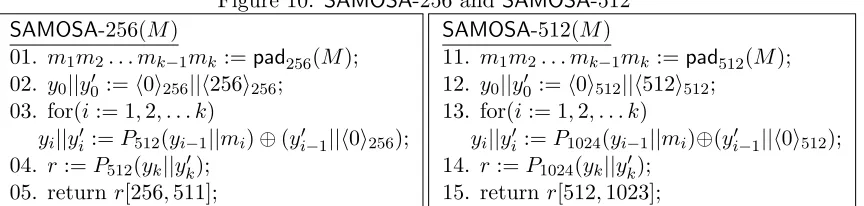
14.1 Description of SAMOSA

(32)

Figure 10: SAMOSA-256 and SAMOSA-512 SAMOSA-256(M)

01. m1m2. . . mk−1mk:=pad256(M); 02. y0||y′0:=⟨0⟩256||⟨256⟩256;

03. for(i:= 1,2, . . . k)

yi||y′i:=P512(yi−1||mi)⊕(yi′−1||⟨0⟩256); 04. r :=P512(yk||yk′);

05. return r[256,511];

SAMOSA-512(M)

11. m1m2. . . mk−1mk:=pad512(M); 12. y0||y0′ :=⟨0⟩512||⟨512⟩512;

13. for(i:= 1,2, . . . k)

yi||yi′ :=P1024(yi−1||mi)⊕(yi′−1||⟨0⟩512); 14. r:=P1024(yk||yk′);

15. returnr[512,1023];

14.2 Security analysis of the SAMOSA family

There are two ways to attack the SAMOSA hash function family: (1) Attacking the FP mode and (2) attacking the underlying permutationP512 orP1024. In the next subsections we present the analysis results on the mode and the permutations. Based on that we conjecture that the SAMOSA family cannot be attacked non-trivially with work less than the brute force.

14.2.1 Security of the FPmode.

In Section 4 we have shown that theFP mode is indiﬀerentiable from a random oracle up to approximately 2n/2 queries (up to a constant factor) where n is the hash size in bits. Our rigorous analysis with the FP mode reveals that it may be possible to improve the bound to nearly 2n queries. The analysis implies that it is hard to attack any concrete hash function based on the FP mode without discovering non-trivial weaknesses in the underlying permutation. In our case, the permutations are P512 and P1024 of the Grøstl hash family.

14.2.2 Security analysis of Grøstl permutations P512 and P1024.

(33)

15 FPGA Implementations of

SAMOSA

-256 and

SAMOSA

-512

15.1 Motivation and previous work

In case the security of two competing cryptographic algorithms is the same or comparable, their performance in software and hardware decides which one of them get selected for use by standardization organizations and industry.

In this section, we will analyze how SAMOSA compares to Grøstl, one of the five final SHA-3 candidates, from the point of view of performance in hardware. This comparison makes sense, because both algorithms share a very significant part, permutation P, but differ in terms of the mode of operation. The FP mode requires only a single permutation P, while Grostl mode requires two permutations P and Q, executed in parallel. Our goal is to determine how much savings in terms of hardware area are introduced by replacing the Grøstl construction for hash function with the FP mode. We also would like to know whether these savings come at the expense of any significant throughput drop. Finally, we would like to analyze how significant is the improvement in terms of the throughput to area ratio, a primary metric used to evaluate the efficiency of hardware implementations in terms of a trade-off between speed and cost of the implementation.

Multiple hardware implementations of Grøstl (and its earlier variant, referred to as Grøstl-0) have been reported in the literature and in the on-line databases of results (see [38], [2]). Most of these implementations use two major hardware architecture types: a) parallel architectures, denoted (P+Q), in which Groestl permutations P and Q are imple-mented using two independent units, working in parallel, and b) quasi-pipeline architec-tures, denoted (P/Q), in which, the same unit, composed of two pipeline stages, is used to implement both P and Q, and the computations belonging to these two permutations are interleaved [16]. Additional variants of each architecture type are possible, and the two most eﬃcient ones are the basic iterative architecture (denoted as x1), and vertically folded architecture, with the folding factor 2 (denoted as /2(v)) [16].