www.geosci-model-dev.net/7/2393/2014/ doi:10.5194/gmd-7-2393-2014
© Author(s) 2014. CC Attribution 3.0 License.
Methods to evaluate CaCO
3
cycle modules in coupled global
biogeochemical ocean models
W. Koeve1, O. Duteil1, A. Oschlies1, P. Kähler1, and J. Segschneider2
1Biogeochemical Modelling, GEOMAR Helmholtz-Zentrum für Ozeanforschung, Düsternbrooker Weg 20,
24105 Kiel, Germany
2Max-Planck-Institut für Meteorologie, Bundesstraße 53, 20146 Hamburg, Germany
Correspondence to: W. Koeve ([email protected])
Received: 21 October 2013 – Published in Geosci. Model Dev. Discuss.: 29 November 2013 Revised: 29 August 2014 – Accepted: 17 September 2014 – Published: 16 October 2014
Abstract. The marine CaCO3cycle is an important
compo-nent of the oceanic carbon system and directly affects the cycling of natural and the uptake of anthropogenic carbon. In numerical models of the marine carbon cycle, the CaCO3
cycle component is often evaluated against the observed dis-tribution of alkalinity. Alkalinity varies in response to the formation and remineralization of CaCO3and organic
mat-ter. However, it also has a large conservative component, which may strongly be affected by a deficient representation of ocean physics (circulation, evaporation, and precipitation) in models. Here we apply a global ocean biogeochemical model run into preindustrial steady state featuring a number of idealized tracers, explicitly capturing the model’s CaCO3
dissolution, organic matter remineralization, and various pre-formed properties (alkalinity, oxygen, phosphate). We com-pare the suitability of a variety of measures related to the CaCO3cycle, including alkalinity (TA), potential alkalinity
and TA∗, the latter being a measure of the time-integrated imprint of CaCO3 dissolution in the ocean. TA∗can be
di-agnosed from any data set of TA, temperature, salinity, oxy-gen and phosphate. We demonstrate the sensitivity of total and potential alkalinity to the differences in model and ocean physics, which disqualifies them as accurate measures of bio-geochemical processes. We show that an explicit treatment of preformed alkalinity (TA0) is necessary and possible. In
our model simulations we implement explicit model tracers of TA0 and TA∗. We find that the difference between
mod-elled true TA∗and diagnosed TA∗was below 10 % (25 %) in 73 % (81 %) of the ocean’s volume. In the Pacific (and In-dian) Oceans the RMSE of A∗is below 3 (4) mmol TA m−3, even when using a global rather than regional algorithms to
estimate preformed alkalinity. Errors in the Atlantic Ocean are significantly larger and potential improvements of TA0 estimation are discussed. Applying the TA∗approach to the output of three state-of-the-art ocean carbon cycle models, we demonstrate the advantage of explicitly taking preformed alkalinity into account for separating the effects of biogeo-chemical processes and circulation on the distribution of al-kalinity. In particular, we suggest to use the TA∗ approach for CaCO3cycle model evaluation.
1 Introduction
According to Sabine et al. (2004), the ocean has taken up about 43 % of the anthropogenic CO2emissions into the
at-mosphere since preindustrial times. The partitioning of CO2
between atmosphere and ocean is controlled by the buffer capacity of the CO2-system in the surface ocean together
with meridional overturning. The buffer capacity of the CO2
-system varies with temperature and the distribution of total inorganic carbon and alkalinity (e.g. Omta et al., 2010, 2011). Biogeochemical processes, namely the organic tissue pump and the CaCO3counter pump, strongly affect the ocean’s
in-ternal cycling and distribution of carbon and alkalinity, which in turn influences the surface ocean buffer capacity and hence the ocean’s ability to take up anthropogenic CO2.
Further-more, the invasion of anthropogenic CO2into the ocean leads
are likely to exist. To better understand and quantify pos-sible global implications of CO2-induced changes in ocean
chemistry, numerical models of marine biogeochemistry and circulation are the method of choice. Data-based model eval-uation is an important step in the development of prognos-tic models suitable for studying the complex interactions of ocean acidification, global warming, ocean biogeochemistry, and their net effect on global ocean carbon uptake and stor-age.
Considerable effort has been devoted to the evaluation of models of the organic tissue pump, i.e. the production, trans-formations, and fluxes of organic matter in the ocean. The distributions of nutrients (e.g. phosphate), oxygen, as well as derived properties like AOU, the apparent oxygen utilization (Pytkowicz, 1971), provide suitable constraints on organic matter fluxes in the ocean (Najjar et al., 2007; Schneider et al., 2008; Kriest et al., 2010; Duteil et al., 2013). These tracers are suitable because the effects of ocean biology on them has a large signal-to-background ratio, i.e. the biotic ef-fect is large compared with other efef-fects. For example, the ra-tio of phosphate remineralized in the interior of the ocean to total observed phosphate ranges between 20 and 45 % in high latitudes and oxygen minimum zones, respectively. This frac-tion can be even higher in shallow waters if preformed phos-phate at the outcrop approaches zero. With AOU the signal-to-background ratio is even more favourable. Were it not for uncertainties in the oxygen saturation assumption required in its computation (Duteil et al., 2013) the effect of biota on AOU would be almost 100 %. The skill of state-of-the-art models to represent the organic tissue pump may hence be well judged from their ability to reproduce the global distri-bution of AOU (Najjar et al., 2007) or the recently suggested Evaluated Oxygen Utilization (EOU, Duteil et al., 2013).
In contrast, evaluating models of the marine CaCO3cycle
is more difficult. Total alkalinity (TA) has frequently been used for this purpose. However, patterns of TA reflect not only the production and dissolution of CaCO3. In this study
we look for adequate tracers which are suited to evaluate the marine CaCO3cycle in biogeochemical models. In Sect. 2
we show that surface ocean patterns of TA are dominated by evaporation and precipitation. Using observations as well as model results we discuss these and other limitations of TA for model evaluation. In Sect. 3 we introduce an approach which has been proposed to explicitly account for non-CaCO3
ef-fects on TA, the TA∗ concept (e.g. Feely et al., 2002). TA∗ measures the time-integrated imprint of CaCO3-dissolution
in the ocean. It is an analogue of AOU, which measures time-integrated oxygen utilization. In Sect. 4 we present our exper-imental approach to test the applicability of TA∗ by means of model simulations, in which computed TA∗is compared with an explicit, idealized, TA∗ model tracer. In Sect. 5 we present and discuss the results of the assessment of TA∗. Fi-nally (Sect. 6), we apply the TA∗approach to real-ocean ob-servations as well as several published models. Note that in this study we assess the suitability of different methods to
evaluate modules of the CaCO3cycle. Applying these
meth-ods to evaluate actual state-of-the-art models, e.g. CMIP5, will be the subject of a future study.
2 TA distribution and CaCO3transformations
The production and dissolution of CaCO3affect the
concen-trations of calcium, total dissolved inorganic carbon (TCO2),
and total alkalinity (TA). However, it is only TA and TCO2
for which the total number of observations and their distribu-tion (GLODAP, Key et al., 2004) can support model evalua-tion on a global scale. The sensitivity of TCO2to production
and dissolution of CaCO3is very low since TCO2is
predom-inately modified by decay of organic matter and influenced by the invasion of anthropogenic CO2. In 99 % of the ocean
interior, organic matter decay has a larger effect on TCO2
than CaCO3dissolution (Fig. 1a). The property (TA-TCO2)
has recently been employed to assess a model’s potential to take up atmospheric CO2(Séférian et al., 2013; Dunne et al.,
2013). This is motivated by the fact that (TA-TCO2) serves
as a good approximation for the carbonate ion concentration at the surface which itself is inversely related to the chem-ical capacity of the ocean to take up CO2 from the
atmo-sphere (Sarmiento and Gruber, 2006; Séférian et al., 2013). In the interior of the ocean (TA-TCO2) is modified by both
the remineralization of organic matter and the dissolution of CaCO3. In the deep ocean (GLODAP data, not shown) the
impact of organic matter remineralization strongly dominates the patterns of (TA-TCO2). On the 2000 m depth plane, for
example, 92 % of the variance of (TA-TCO2) is explained
by variations of AOU. The property (TA-TCO2) is hence not
suitable to assess a model’s CaCO3cycle.
The effect of CaCO3 dissolution on TA exceeds that of
organic matter remineralization in about 60 % of the ocean volume (Fig. 1b) making TA more appropriate to evaluate CaCO3 models. Therefore TA is often used as a data
con-straint in global CaCO3modelling (e.g. Gehlen et al., 2007;
Ilyina et al., 2009; Ridgwell et al., 2007). A major con-cern, however, in using TA concentrations for data-based model evaluation is the fact that it has a large background. In the deep North Pacific Ocean, where the largest time-integrated imprint of CaCO3dissolution is observed (about
120 mmol TA m−3, Feely et al., 2002), it is equivalent to 5 % of the observed TA only. Everywhere else the contribution of CaCO3dissolution on TA is even lower. On a global average,
the ratio of the CaCO3-dissolution imprint to TA-background
is about 0.02. The global mean ratio of the alkalinity effect stemming from organic matter remineralization to TA back-ground is only 0.005. Contributions from N2-fixation,
Figure 1. Ratio of the imprint of the organic tissue pump and the CaCO3 pump on TCO2 (a) and TA (b) at 2000 m water
depth.1DICtissue and1TAtissueare computed from estimates of the apparent oxygen utilization (AOU) and the mean molar oxy-gen : carbon ratio of 1.4 and the mean molar oxyoxy-gen : alkalinity ratio of 0.119 (=1/170×16×1.26), respectively. AOU is esti-mated using oxygen, potential temperature and salinity data from the World Ocean Atlas (gridded data, analysed annual means).
1TACaCO3 is computed using the TA∗method described in Sect. 3 applied to the GLODAP gridded data set (Key et al., 2004).
1DICCaCO3=0.5×TA∗.
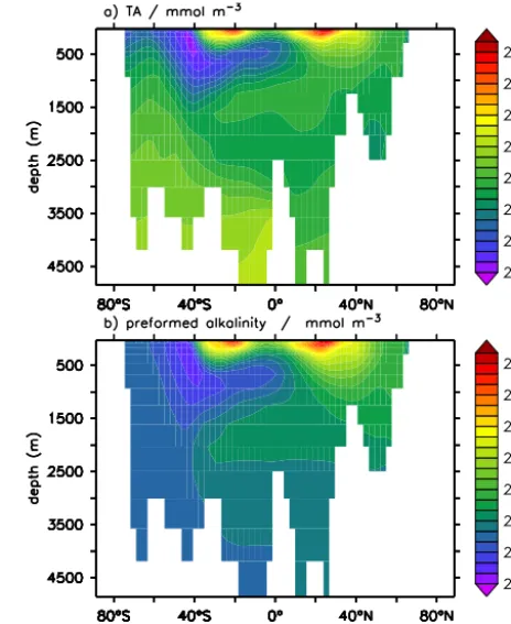
GLODAP data composite is explained by salinity variation (Fig. 2). This is easily understood since alkalinity represents the charge balance of the major constituents of sea salt, and like salinity, surface ocean alkalinity is largely determined by evaporation and precipitation (e.g. Friis et al., 2003). In the ocean interior its distribution is largely explained by advec-tion and mixing of “preformed alkalinity” (Fig. 3a and b). In analogy to the concept of preformed nutrients or preformed oxygen (Redfield et al., 1963; Duteil et al., 2012, 2013), preformed alkalinity (in the following denoted TA0) refers to the alkalinity which a water mass had when last in con-tact with the atmosphere before being subducted (Chen and Millero, 1979). In the ocean interior TA0 is a strictly con-servative tracer, whereas TA is variable due to transforma-tions of CaCO3and organic matter. These principles apply
both to models and the real ocean, yet there is the difficulty that in the real ocean TA0cannot be separated from TA by
Figure 2. Surface ocean distribution of TA (a, GLODAP, gridded data, http://cdiac.ornl.gov/ftp/oceans/GLODAP_Gridded_ Data/, last access: 10 December 2009) and salinity (b, World Ocean Atlas, WOA, analysed annual means, Antonov et al., 2010). The scaling of the isolines was chosen to emphasize the global linear relationship between alkalinity (µmol kg−1) and salinity. With ungridded bottle data from the upper 100 m of the ocean (GLODAP/WAVES data set, http://cdiac3.ornl.gov/ waves/discrete/, last access: 31 March 2012) this relationship is TA=699.75+46.18·S;r2=0.71.
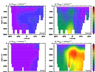
measurements. In a model, the distribution of TA0 can be studied by designing an explicit tracer of TA0 (see Sect. 4 for details). Along a section at 30◦W in the Atlantic (Fig. 4), the range of modelled TA0 values is equivalent to 97 % of the range of modelled TA; along a section at 150◦W in the Pacific (not shown) the respective value is 69 % in our model (see Sect. 4 for a description of the model). Given that phys-ical processes can never be represented perfectly in coupled biogeochemical circulation models (e.g. Doney et al., 2004), it is not recommended to use the distribution of bulk TA as a descriptor of CaCO3transformations in a data–model
com-parison. Small deficiencies in the representation of TA0, e.g. due to errors in the surface salinity balance, or errors in ocean circulation and mixing, can have profound effect on TA dis-tribution in the ocean interior. Apparently good (Fig. 5a) or bad (Fig. 5c and d) fits of model and observed TA (Fig. 5b) may hence betray our judgement of the respective CaCO3
Figure 3. Horizontal sections of alkalinity (a, GLODAP) and salin-ity (b, WOA) along 30◦W in the Atlantic Ocean. For the scaling of the isolines see caption of Fig. 2. Alkalinity patterns, particularly in the upper 2000 m, largely follow patters of salinity indicating a pre-dominantly conservative behaviour of alkalinity in the interior of the Atlantic Ocean. Ther2of (a) over (b) is 0.692.
Recognizing these shortcomings of using TA patterns to estimate CaCO3cycling, different approaches have been
pro-posed to overcome them. For example, Howard et al. (2006), suggested a tracer Alk∗=Alk−Alkmean/Smean· S, with AlkmeanandSmeanbeing the oceanwide means of alkalinity and salinity, respectively. Variation of this Alk∗tracer in the deep ocean is supposed to be driven by CaCO3dissolution
(increase in alkalinity) and the remineralization of organic matter (decrease in alkalinity) only (Howard et al., 2006). (For the purpose of not confusing Howard’s Alk∗tracer with other tracers we use in our study, we rename their Alk∗ as TAH06=TA−TAave/Save· S.) The emerging pattern of
this tracer along a transect in the Atlantic (Fig. 6a) suggests a dominance of CaCO3 production (and/or organic matter
remineralization) in the North Atlantic and of CaCO3
dis-solution in waters originating from the Southern Ocean. Ap-plying Howard’s approach to our model tracer TA0, we com-pute the anomaly TA0−TA0ave/Save · S. As the TA0 tracer
behaves conservatively within the ocean, its anomaly should not reflect any local effects of either CaCO3dissolution or
or-ganic matter remineralization. However, the patterns of this anomaly in our model simulation (Fig. 6b) are very similar to the pattern of the Howard et al. (2006) tracer (Fig. 6a) itself,
Figure 4. Distribution of total alkalinity (a) and a preformed alka-linity tracer (b) along 30◦W from a model run (TMM-MIT28, see Sect. 4 for details of the model experiments). Ther2of (a) over (b) is 0.631. The preformed alkalinity (TA0) tracer is restored at the surface and at any time step of the model run to total alkalinity. In the interior of the model ocean TA0has no biogeochemical sources or sinks but is advected and mixed conservatively. TA in this model is affected by both physical and biogeochemical processes.
indicating that the Howard et al. (2006) tracer is not informa-tive about where and how much CaCO3dissolves.
Another property suggested as a tracer of CaCO3
transfor-mations, which excludes any effects of salinity and organic tissue production or remineralization, is Potential Alkalinity (PALK=(TA +NO3)/S· 35, e.g. Sarmiento et al., 2002).
Here, the salinity normalization is to correct for the effects of the freshwater balance and the nitrate term is to com-pensate for the alkalinity effects of organic matter dynam-ics. Yet again, modelled patterns of both PALK and PALK0 =( TA0+PO40· 16)/S· 35) in the Atlantic (Fig. 6c, d)
trace characteristic water masses observed in the Atlantic Ocean, like North Atlantic Deep Water, Antarctic Interme-diate Water and Antarctic Bottom Water conservatively. Pat-terns of PALK can hence not straightforwardly be interpreted in terms of the local process of CaCO3dissolution or
produc-tion.
2250 2300 2350 2400 2450 2500 25500 10
20 30
Alkalinity (mmol / m3)
Volume Fraction (%)
PISCES
2250 2300 2350 2400 2450 2500 2550
Alkalinity (mmol / m3)
HAMOCC 0
10 20 30
Volume Fraction (%)
UVICï2.8 GLODAP
(a) (b)
(c) (d)
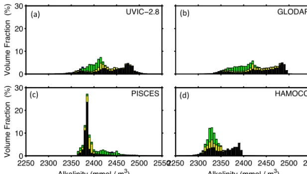
Figure 5. Global ocean volume-weighted frequency-distribution of alkalinity in observations (GLODAP data set, Key et al., 2004) and three global carbon cycle models (see Duteil et al., 2012 for details). Fractions of the Atlantic, Pacific, Indian and Arctic Oceans are indicated by colour codes (green, black, yellow and blue, respectively).
(Robbins, 2001; Friis et al., 2003), which are highly vari-able on a global scale. In the Atlantic, for example, riverine zero-salinity alkalinity ranges from about 250 (Amazon) to 2500 (Mississippi) mmol m−3(e.g. Cai et al., 2010). Fresh-water alkalinity depends on geochemical conditions of the respective drainage basins. In models, zero-salinity alkalin-ity end members depend on model-specific alkalinalkalin-ity ocean-boundary conditions. However, neither of these effects can explain the distribution of PALK and PALK0in the ocean’s
interior of our model simulation. Here, two additional prob-lems of the PALK concept become obvious: the biogenic modifications of TA in the surface ocean and, in particular, the recirculation of TA in the Southern Ocean. CaCO3
pro-duction in the surface ocean changes TA and consequently affects TA0. The PALK concept does not correct for this ef-fect and hence the imprint of surface CaCO3production
trav-els with PALK and PALK0through the interior of the ocean where, being subject to mixing, it complicates the interpreta-tion of PALK with respect to CaCO3dissolution. Concerning
the PALK (and TAH06) patterns in the South Atlantic (Fig. 6), however, the recirculation of TA is likely to be most impor-tant. The Southern Ocean is the major site where deep wa-ter returns to the surface (Marshall and Speer, 2002). Wa-ter which has accumulated the imprint of CaCO3dissolution
in the North Pacific returns to the surface in the Southern Ocean. Subsequently, most of this water is re-injected into the interior of the ocean either as Antarctic Intermediate Wa-ter or Antarctic Bottom WaWa-ter. Similarly, the imprint of oxy-gen utilization in the ocean’s interior wells up in the Southern Ocean, indicated by significant oxygen undersaturation there (Ito et al., 2004). Gas exchange with the atmosphere, how-ever, is able to reset oxygen to values corresponding to sur-face temperature and salinity nearly completely. But for TA no equivalent restoring process to reset it to values consistent
with actual surface salinity exists. The PALK pattern ob-served in the South Atlantic must hence be interpreted as a recirculation of the imprint of CaCO3 dissolution having
taken place as far away as the North Pacific. We conclude that neither TA data nor derivatives like TAH06or PALK are well suited for the data-based evaluation of ocean CaCO3
cycle models. Computing the difference between PALK and PALK0(Anonymous, 2013) leads us to a property which has been used for the quantification of CaCO3dissolution.
Ignor-ing the effect of denitrification and assumIgnor-ing N/P and O2/P
ratios of 16 and 170, this difference can be rewritten as (TA− TA0+NO3−NO03)/S·35=(TA−TA0+NO3remin)/S·35.
In this way the imprint of CaCO3dissolution would be
com-puted from observed TA, an explicit estimate of preformed TA, and an estimate of the alkalinity effect of organic mat-ter remineralization. In the next section we describe TA∗, a similar property, suggested earlier as a measure of the time-integrated effect of CaCO3 dissolution in the ocean (Feely
et al., 2002; Sabine et al., 2002; Chung et al., 2003).
3 TA∗approach
The TA∗ approach (Feely et al., 2002; Sabine et al., 2002; Chung et al., 2003) has been used to quantify the time-integrated imprint of CaCO3 dissolution. Variants of this
method have been vital for the determination of anthro-pogenic CO2in the ocean since the early paper of Chen and
Millero (1979). The underlying concept (Eq. 1) of the TA∗ approach is that the observed alkalinity (TA) in the interior of the ocean is composed of a preformed component, TA0, a term caused by the remineralization of organic matter, TAr, and a term due to CaCO3 dissolution, usually coined TA∗
Figure 6. Anomalies of TA (a) and TA0 (b) and the respective salinity normalized properties. (c) Potential alkalinity PALK=(ALK+PO4·16)/S·35 distribution along a section through the Atlantic. (d) Potential preformed alkalinity PALK0=(TA0+
PO40·16)/S·35. The distribution along 30◦W from a model run (TMM-MIT28, see Sect. 4 for details of the model experiments) is shown.
below, all terms are in units of mmol TA m−3):
TA = TA0+TA∗−TAr. (1)
Remineralization of organic matter, through the regen-eration of nitrate, phosphate and sulfate, decrements TA while the dissolution of CaCO3 increments it
(Wolf-Gladrow et al., 2007). The alkalinity effect of organic matter decomposition can be parametrized as a function of AOU, i.e. TAr=rAlk:NO3 · rNO3: −O2 · AOU. Values for rNO3: −O2 and rAlk:NO3 are usually derived from observa-tions, e.g. rNO3: −O2=1/10.625, rAlk:NO3=1.26 (Ander-son and Sarmiento, 1994; Kanamori and Ikegami, 1982), and are generally prescribed in biogeochemical models. Considering maximum values of AOU observed in the ocean (about 350 mmol O2m−3), the largest TAr is about
40 mmol TA m−3. The global average TAr(using AOU from the World Ocean Atlas) is 18.1 mmol m−3. Considering AOU to overestimate true oxygen utilization by 20–25 % (Ito et al., 2004; Duteil et al., 2013), TArcomputed from AOU is probably also overestimated accordingly.
Preformed alkalinity denotes the alkalinity, which a wa-ter parcel had during its last contact with the atmosphere (Chen and Millero, 1979). Since all water masses in the in-terior of the ocean are mixtures of various end-members, the preformed alkalinity is also a mixture of different end-member alkalinity concentrations. For a given location in the ocean interior, neither the preformed alkalinity end-member concentrations nor their mixing ratios are known. Preformed
alkalinity, TA0, must therefore be diagnosed. This is usually done by an empirical approach which comprises two steps (e.g. Feely et al., 2002; Matsumoto and Gruber, 2005. First, a multi-linear regression of alkalinity with salinity, tempera-ture and PO (or NO) is derived from near-surface data: TAsurf=a0+a1· Ssurf+a2· Tsurf+a3· POsurf. (2)
PO (or NO) are considered conservative tracers within the ocean (Broecker, 1974) and defined as PO=O2+r−O2:PO4·PO4, and NO=O2+r−O2:NO3·NO3, assuming that r−O2:PO4 and r−O2:NO3 are constant in the interior of the ocean (r−O2:PO4=170; r−O2:NO3=10.625; Anderson and Sarmiento, 1994). Secondly, the coefficients derived from surface data are subsequently applied to salinity, potential temperature and PO (or NO) data from the interior of the ocean to compute TA0everywhere:
TA0(x, y, z)=a0+a1· S(x, y, z)
+a2·potT(x, y, z)+a3· PO(x, y, z). (3)
4 Modelling approach
Although variants of the TA∗ method have been in use for
decades there has, to our knowledge, not been any explicit and quantitative assessment of this method. The main reason for this is that in the real ocean no independent and rigorous approach to quantify the imprint of CaCO3-dissolution
ex-ists. Hence the potential and limitations of the TA∗-method have never been tested. Here, we apply a prognostic global ocean carbon cycle model for this purpose. The model con-sists of an offline representation of ocean physics providing transport and mixing within the ocean, a NPZD-type model to represent the organic tissue pump, a CaCO3cycle module,
as well as idealized tracers of TA0, TA∗and TAr.
For the physical model we use the transport matrix method (TMM) described in detail by Khatiwala et al. (2005) and Khatiwala (2007). In this approach, passive tracer transport is represented by a matrix operation involving the tracer field and a transport matrix extracted from the MIT general cir-culation model, a primitive equation ocean model (Marshall et al., 1997). Seasonally cycling (monthly) coarse-resolution matrices were derived from a 2.8◦×2.8◦global configura-tion of this model with 15 layers in the vertical, forced with monthly mean climatological fluxes of momentum, heat and freshwater, and subject to a weak restoring of surface temper-ature and salinity to observations. The same transport matri-ces were employed by Kriest et al. (2012) in their data-based assessment of biogeochemical models.
The model of the organic tissue pump used with the TMM is the NPZD–O2–DOP model of Schmittner et al. (2005) as
modified by Kriest et al. (2010, 2012). The primary model currency is phosphorus (phosphate, DOP, phytoplankton, zooplankton, detritus) with oxygen as an additional model tracer. The molar O2:P ratio is fixed at 170 (Anderson and
Sarmiento, 1994). Sinking and remineralization of detritus are parametrized by a combination of a constant remineral-ization rate and particle sinking speeds increasing with depth, together reflecting a power-law function of the flux profile (Martin et al., 1987) with an exponent of 1.075 (Kriest et al., 2010). The latter value has been found to yield global oxygen and phosphate distributions in good agreement with observa-tions (Kriest et al., 2012).
In order to represent oceanic alkalinity in a pragmatic way we implement the tracer TA and couple the production and remineralization of organic matter with fixed ratios to the uptake and release of phosphate in the NPZD–O2–DOP
model. We use a TA:P ratio of 21.8. CaCO3 is produced
with a temperature-dependent inorganic carbon : organic car-bon ratio bound to the rate of detritus production in the model. The global CaCO3 export production of our model
is 0.9 Gt C year−1, similar to other models and observational estimates (Berelson et al., 2007). In our model, CaCO3
ex-port and dissolution are instantaneous and follow an expo-nential decay function with a decay length scale of 2000 m. Although this may not be a mechanistic representation of the
processes involved in CaCO3 dissolution, it is a pragmatic
parametrization. It has previously been used e.g. in the UVIC model (see Sect. 6 below for a brief description of the mod-els employed), which yield TA-distributions (Fig. 5) and TA∗ global mean profiles (Sect. 6) in good agreement with obser-vations. We present preindustrial Holocene steady-state re-sults from a model run over 6000 years of model integration.
4.1 Idealized tracers
We implement a number of idealized tracers. The tracer of preformed alkalinity, TA0, is restored to model TA every-where at the surface and at every time step. In the inte-rior of the model ocean this tracer has no sinks or sources, but is transported and mixed conservatively according to our model’s physics. The TA∗tracer is set to zero at the surface.
In the interior of the model ocean this tracer collects the effect of CaCO3 dissolution whenever it occurs. Similarly,
a TArtracer is set to zero at the surface and collects the alka-linity effect of organic matter remineralization in the ocean interior. All idealized tracers are transported and mixed ac-cording to model physics. In this way, we perfectly know TA0, TA∗and TArat any point and time in the model. It is run for 6000 years until practically at each grid point the sum of the idealized tracers equals the model’s TA, i.e. Eq. (1) is satisfied. In order to test the TA∗ concept we compare the model tracers TA0and TA∗(in the following denoted TA0true and TA∗true) with these two properties as diagnosed from the model TA, PO4,T,S, O2, and AOU, according to Eqs. (1)–
(3). In the following the diagnosed properties are denoted TA0diagand TA∗diag, respectively.
4.2 TA0algorithms
ocean PO do not behave conservatively over the seasonal cy-cle. Temperatures are higher in summer than in winter and, because of temperature-induced outgassing of oxygen, PO is lower in summer. It may therefore be speculated that TA0 al-gorithms derived from seasonally biased surface data do not predict interior ocean TA0reliably. We test this by deriving algorithms based on sampling the surface ocean of our model either seasonally unbiased, summer biased or winter biased. The expectation is that winter-biased TA0algorithms should provide the best predictions of TA∗. In order to derive the seasonally unbiased TA0algorithms we sample monthly re-solved model output during every month and at every grid box at the surface. For the seasonally biased sampling, we use the same model output but sampled only during the given season of the respective hemisphere. We defined winter as January–March (July–September) in the Northern (Southern) Hemisphere.
5 TA∗method assessment
In the following we compare the model’s true TA∗ (TA∗true being the TA∗tracer) with TA∗diagestimated from the model output (according to Eqs. 1 to 3). Using TA∗trueas a reference we compute volume weighted RMSEs of TA∗diagaggregated on global and basin scales and for different depth levels, i.e. RMSE =
v u u t "
X
i,j,k
voli,j,k/voltotal×
TA∗diag− TA∗true2
i,j,k
#
. (4)
We apply this approach to different sets of diagnosed TA∗ which are distinguished by the different seasonally biased estimates of TA0(see previous section). In order to isolate the error related to the computation of TA0 we here ignore any error related to the estimation of TAr from diagnosing AOU and use the explicit model tracer of TArwhen comput-ing TA∗, i.e. TA∗
diag=TA−TA 0 diag+TA
r true.
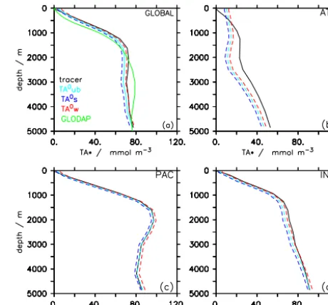
Using a single global algorithm (Table 1, #1) derived from the seasonally unbiased sampling of surface ocean data for the computation of preformed alkalinity (TA0ub), we can re-produce the TA∗truedistribution relatively well: the global av-erage volume-weighted RMSE of TA∗ in the interior of the ocean (below 100 m) is 5.8 mmol m−3(Table 2, #1) and the global mean profiles of TA∗diag and TA∗true show very sim-ilar vertical patterns, while TA∗diag is generally somewhat smaller than TA∗
true(Fig. 7a). The performance of the global
algorithm varies with ocean basin, with RMSEs as low as 2.8 mmol m−3 and as high as 10.4 mmol m−3in the Pacific and Atlantic oceans, respectively (Table 2). Using TA0 algo-rithms derived from regional data reduces the RMSE slightly in the Atlantic and Indian Oceans, while increasing it in the Pacific Ocean. The surface alkalinity RMSE (column 2 in Table 2) has little predictive power for the RMSE of TA∗
Figure 7. (a) Global mean profile of TA∗from explicit model tracer (black, solid) and computed from model data (dashed). The two dashed lines are based on seasonally biased sampling of the model output at the surface when deriving the TA0algorithm. TA0s refers to sampling during summer, TA0wrefers to winter sampling when deep water actually forms. TA0ubrefers to seasonally unbiased sam-pling. For comparison, the green line shows the global mean profile of TA∗computed from the GLODAP database and using a globally uniform algorithm derived from the gridded surface GLODAP data (b–d). Basin-averaged profiles of TA∗for the Atlantic, Pacific and Indian oceans. Tracer-based estimate (black, solid) and computed TA∗from winter- and summer-biased TA0algorithms are shown.
in the interior of the ocean. Basin-averaged vertical profiles (Fig. 7b–d), show excellent agreement of diagnosed and true TA∗in the Pacific while in the Atlantic, TA∗
diagis an
underes-timate of TA∗true. Basin-averaged vertical profiles of the TA∗ RMSE (Fig. 8a) are rather uniform in the Pacific and In-dian oceans and have subsurface maxima at 2000 m depth in the Atlantic Ocean. The basin-average relative error of TA∗ is 10 % or less in the Pacific and Indian oceans below about 1000 m water depth (Fig. 8c). In the Atlantic Ocean the relative error (TA∗RMS/TA∗·100) is higher throughout
and above 30 % in most of the water column, because of large RMSEs and low TA∗signal strength (Fig. 8b).
Using seasonally biased surface data to derive the TA0 al-gorithms yields increased TA∗ RMSEs for summer-biased
sampling and usually slightly reduced TA∗ RMSEs for
Table 1. TA0algorithms. Algorithms are derived from surface data (upper 100 m) of the model. Subsets “winter data” “summer data”) use surface data from winter (summer) months of the respective hemispheres only. Basin-specific algorithms are based on data from the respective ocean basin.
# Subset Equation
Global
1 All months TA0=370.5765+54.0812·S+0.3804·T+0.1129·PO 2 Winter data TA0=357.9100+54.3812·S+0.3824·T+0.1130·PO 3 Summer data TA0=336.2851+55.0656·S+0.4047·T+0.1167·PO
Atlantic
4 All months TA0=263.3001+56.1655·S+1.4997·T+0.1702·PO 5 Winter data TA0=122.0885+59.9151·S+1.5293·T+0.1857·PO 6 Summer data TA0=323.8251+54.4048·S+1.6823·T+0.1737·PO
Pacific
7 All months TA0=559.3595+49.0273·S+0.0923·T+0.0861·PO 8 Winter data TA0=550.7772+49.3419·S−0.0299·T+0.0794·PO 9 Summer data TA0=506.9215+50.5235·S+0.1332·T+0.0903·PO
Indic
10 All months TA0=844.9869+40.6930·S+0.0261·T+0.0960·PO 11 Winter data TA0=715.8663+44.1346·S+0.2181·T+0.1095·PO 12 Summer data TA0=824.6536+41.4498·S−0.1242·T+0.0902·PO
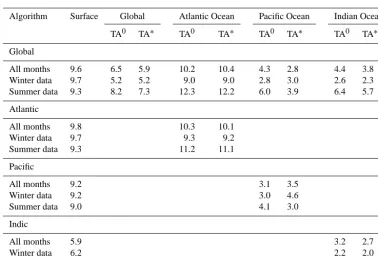
Table 2. Volume-weighted RMSEs of global and regional TA0and TA∗estimates. Errors given in column “Surface” refer to the ability of the respective algorithm to reproduce the surface (upper 100 m) alkalinity of the model. Under TA0RMSEs of subsurface preformed TA as compared with TA0from the explicit tracer are given. Under TA∗RMSEs of computed TA∗compared with TA∗from the explicit tracer are given. Global algorithms are also evaluated concerning their skill on regional scales.
Algorithm Surface Global Atlantic Ocean Pacific Ocean Indian Ocean
TA0 TA∗ TA0 TA∗ TA0 TA∗ TA0 TA∗
Global 9.6 6.5 5.9 10.2 10.4 4.3 2.8 4.4 3.8
Atlantic 9.7 10.3 10.1
Pacific 9.2 3.1 3.5
Indic 5.9 3.2 2.7
TA∗ RMSEs there. It is worth noting that despite the large RMSEs, diagnosed TA0still resembles the overall regional patterns of true TA0 in the interior of the Atlantic Ocean (Fig. 9). We speculate that this is caused by the complex mix-ture of waters subducted in the north and south with their different end-member properties. Neither the global nor the basin-scale TA0algorithm can predict TA0in the interior of the Atlantic Ocean well enough to allow reasonable TA∗ es-timates. This is also reflected by particularly large RMSEs of the TA0estimate in the North Atlantic Deep Water (NADW) (Fig. 9d), where the TA0algorithm overestimates TA0by 10– 14 mmol m−3(Fig. 9c).
Zonal averages of TA∗
truein the Pacific and Atlantic oceans
are compared with the difference of diagnosed and true TA∗
(Fig. 10). In intermediate waters of the Atlantic, but also in
the North Atlantic Deep Water, uncertainties of TA∗are of similar magnitude as TA∗. It is only in Antarctic Bottom Water that uncertainties are small enough to detect TA∗ in the Atlantic. In the Pacific the picture is quite different. TA∗ is detectable almost everywhere except in surface and mode waters of the upper several hundreds of metres.
As a note of caution it is stressed again that TA∗is a time-integrated property subject to advection and mixing. The oc-currence of a large TA∗values at a given location does not necessarily indicate the rate of CaCO3dissolution to be
par-ticularly large there. This characteristic of TA∗is shared with many other cumulative properties, notably AOU, which rep-resents the time-integrated measure of remineralization of or-ganic matter, not its actual, local rate. The observation of TA∗
Figure 8. Basin-average vertical profiles of TA∗RMSE (a), TA∗(b) and the percent ratio of the two (c). Blue solid: Atlantic Ocean. Red dashed: Pacific Ocean. Black dashed: Indian Ocean.
Table 3. Volume-weighted RMSEs for TA0and TA∗estimates based on seasonally unbiased TA0algorithm (all months) and winter- and summer-biased algorithms respectively. Column “surface” refers to the skill of the respective algorithm to reproduce the surface (upper 100 m) alkalinity of the model. Column TA0gives RMSEs of subsurface preformed TA as compared with TA0from the explicit tracer. Column TA∗gives the RMSE of computed TA∗compared with TA∗from the explicit tracer. Global algorithms are also evaluated concerning their skills on regional scales.
Algorithm Surface Global Atlantic Ocean Pacific Ocean Indian Ocean
TA0 TA∗ TA0 TA∗ TA0 TA∗ TA0 TA∗
Global
All months 9.6 6.5 5.9 10.2 10.4 4.3 2.8 4.4 3.8
Winter data 9.7 5.2 5.2 9.0 9.0 2.8 3.0 2.6 2.3
Summer data 9.3 8.2 7.3 12.3 12.2 6.0 3.9 6.4 5.7
Atlantic
All months 9.8 10.3 10.1
Winter data 9.7 9.3 9.2
Summer data 9.3 11.2 11.1
Pacific
All months 9.2 3.1 3.5
Winter data 9.2 3.0 4.6
Summer data 9.0 4.1 3.0
Indic
All months 5.9 3.2 2.7
Winter data 6.2 2.2 2.0
Summer data 5.4 5.1 4.4
minerals of CaCO3, calcite and aragonite, respectively, has
sometimes erroneously been interpreted to indicate shallow CaCO3dissolution – see Friis (2006) and Friis et al. (2007)
for a discussion. Here we show that, in addition, TA∗in these waters usually cannot be determined accurately due to uncer-tainties in the TA0estimate.
6 Application of the TA∗ approach to GLODAP and three OCMIP5 models
Finally, we apply the TA∗approach to an observation-based
data product and to the output from three different mod-els available at the Ocean Carbon Cycle Model Intercom-parison Project data server (http://ocmip5.ipsl.fr; accessed April 2012). Note that this is not the output from the CMIP5 exercise, e.g. for MPI-ESM it is from C4MIP. As for the ob-servations, we combine the GLODAP gridded data set of TA (Key et al., 2004) withT,S, PO4and O2from the annual
Figure 9. TA0distribution in the Atlantic Ocean from explicit tracer (a) and computed from winter biased surface sampling (b). Panel (c) shows the anomaly between the two and panel (d) the basin average RMSE of TA0.
Figure 11. Global mean profiles of (a) TA, (b) TA0, (c) TA∗and (d) TArin the GLODAP data set and in three different models. Prop-erties in (b–d) are diagnosed according to the methods described in Sect. 3. For each of the data sets a specific TA0algorithm was derived from annual mean data (models) or the annual compos-ite GLODAP data, respectively (see text for details and insert for colour code of the models and data used).
et al., 2009). As for the models, we use output prepared for the control runs. Specifically, we use the first available annual time slice of either the CTL or HIST runs, repre-senting the end of the respective model spin-up. We use output of the IFM/UVIC2-8 (Oschlies et al., 2008; http:// ocmip5.ipsl.fr/models_description/ifm_uvic2-8.html), MPI-ESM with the marine carbon cycle component HAMOCC (Maier-Reimer et al., 2005; see also http://ocmip5.ipsl.fr/ models_description/mpi-m_cosmos.html) and IPSL/IPSL-CM4 (Aumont and Bopp, 2006; see also http://ocmip5.ipsl. fr/models_description/ipsl_ipsl-cm4.html) models. It is be-yond the scope of this paper to provide a full evaluation or model intercomparison of the three models. Instead we focus on a comparison of global mean profiles of TA, TA0, TArand TA∗from the three models and the observations with the only objective to illustrate the advantage of explicitly accounting for preformed alkalinity in a data-based model evaluation.
The global mean profile of alkalinity in the observations is characterized by an absolute minimum at the surface, a shal-low maximum at about 100 to 200 m, a subsurface minimum at about 500 m, and a broad maximum between 3000 m and the bottom (Fig. 11a). The three models reproduce this struc-ture to different degrees. The UVIC2-8 tracks the overall ver-tical gradient well while not reproducing the small-scale sub-surface structures. The MPI-ESM tracks the vertical struc-ture well, albeit with a too small overall vertical gradient, but
has a clear negative offset of about 80 mmol m−3. This
off-set is due to losses to the sediment during the model spin-up. The IPSL-CM4 shows too high a TA in the upper 1000 m and too low a TA in the deep ocean by up to 40 mmol m−3 each. Subdividing TA into its components (TA0, TA∗ and TAr) indicates that much of the misfits or fits between the global mean profiles of the individual models and the data are due to differences in preformed alkalinity (Fig. 11b). This is the case for the negative offset of the MPI-ESM model, the wrong surface-to-deep gradient in IPSL-CM4, as well as the good agreement between UVIC2-8 and GLODAP con-cerning the surface-to-deep gradient and the overall shape of the vertical profiles. The subsurface shallow maxima and minima in the observed TA global profile are due to pre-formed TA0only, and they are not related to biogeochemical modifications of alkalinity. TAr(Fig. 11d) as diagnosed from AOU global mean profiles shows small differences between models and data, in agreement with our expectations (see Sect. 5) that uncertainties in TArcontribute little to uncertain-ties in the computation of TA∗. The global mean profiles of TA∗(Fig. 11c) suggest more agreement between models (and data) as might have been guessed from the global mean pro-files of TA (Fig. 11a) alone. Yet, the globally integrated TA∗ inventory of IPSL-CM4 and MPI-ESM is about 25 % smaller than in both the GLODAP and the UVIC2-8 model. Also the distribution of TA∗with respect to CaCO3saturation states
varies considerably between models and observations (Ta-ble 4). In IPSL-CM4 and MPI-ESM, the models which un-derestimate global CaCO3 dissolution, about two-thirds of
the integrated TA∗is found in waters whereCA, the degree
of saturation with respect to calcite is less than 1, while much smaller fractions are observed in waters with higher satu-ration. In GLODAP data the former fraction is about 55 % while the UVIC model has only 43 % of integrated TA∗in undersaturated water. A large fraction of TA∗ in undersatu-rated water is in agreement with expectations from dissolu-tion chemistry (e.g. Morse and Arvidson, 2002) and obser-vations from the ocean where undersaturated waters in the North Pacific show the largest TA∗(Feely et al., 2002). Over-all, differences between observations and models both in the global integral of TA∗and its distribution point to larger un-certainties in the CaCO3 modules of coupled carbon cycle
models than their organic tissue pump modules: on a global scale the time-accumulated imprint of organic matter rem-ineralization on the oxygen distribution as measured by the AOU of several state-of-the-art models agreed within±10 % with observed AOU (Duteil et al., 2013; see also Fig. 11d).
The metric TA∗ allows us to compare the patterns of the
imprint of CaCO3dissolution between models and the ocean.
Hence, it may be used to identify the model which fits obser-vations best. In the example of the three models compared it is the UVIC model which shows the most appropriate global mean profile of TA∗ (Fig. 11) and also the best fit of TA∗ patterns relative to CaCO3 saturation (Table 4). The latter,
Table 4. Global TA∗inventories (Pmol C) and its fractions with respect to the CaCO3saturation states.
Model Global TA∗ inventory (P mol C)
OmegaCa<1 (%)
OmegaCa≥1 and
OmegaAR<1 (%)
OmegaAr≥1 (%)
GLODAP 38.9 55.3 41.3 3.4
IFM-UVIC28 40.0 43.0 49.1 7.9
IPSL-CM4 29.3 71.7 13.7 14.6
MPI-ESM 28.7 67.8 21.7 10.5
GLODAP is not defined north of 65◦N. Model inventories and fractions are computed using the ocean volumes of the
given model and the omega distribution in the respective models.
UVIC model applies the least mechanistic formulation of CaCO3 dissolution of the three models. Both in the
IPSL-CM4 and the MPI-ESM models, CaCO3dissolves
depend-ing on CaCO3 undersaturation (Maier-Reimer et al., 2005;
Aumont and Bopp, 2006), known as the dominant factor of CaCO3dissolution (Morse and Arvidson, 2002). The UVIC
(Oschlies et al., 2008) instead applies an exponential decay function which dissolves CaCO3 independent of the
satu-ration state. To improve a model’s mechanisms of CaCO3
dissolution obviously does not (necessarily) improve its per-formance relative to an evaluation metric. The reasons for this are manifold. For any time-integrated property (like TA∗ or AOU) the age structure of the model is particularly rele-vant. Models with more sluggish deep water circulation will tend to show elevated ages (time since last contact with the atmosphere). With more time to accumulate the imprint of CaCO3dissolution or organic matter decay such models will
also be characterized by higher TA∗ or AOU, in particular in the deep ocean. For this reason an analysis of the model age structure using suitable tracers (Koeve et al., 2014) is a fundamental element of model evaluation. Also, the absolute amount and horizontal patterns of CaCO3production affect
the distribution of TA∗. This can well be compared between models, but like other biogeochemical rates is not well con-strained in the real ocean. Considering CaCO3dissolution in
models with saturation-dependent dissolution formulations (e.g. IPSL-CM4, MPI-ESM), production patterns of organic matter together with the age structure control the patterns of AOU and thereby of respiratory carbon. This is a major deter-minant of CaCO3undersaturation in the deep ocean. Hence,
in these models organic-matter-related processes have a sig-nificant impact on TA∗. Also, the representation of CaCO3
dissolution or burial in sediments (Dunne et al., 2012) may be of importance. Both the IPSL-CM4 and the MPI-ESM model contain a simple sediment module while the UVIC does not. The focus of this study is the assessment of the TA∗method and not the evaluation of individual models which requires to disentangle the interactions of the different drivers of the TA∗ distribution. We leave this to a follow-up paper which will
apply the TA∗ method in the framework of CMIP5 model
analysis.
7 Conclusions
In this study we tested the applicability of the TA∗approach (Feely et al., 2002) to quantify the time-integrated and ad-vected signal of CaCO3dissolution in models and
observa-tions by means of an ocean carbon cycle model augmented with idealized tracers of CaCO3dissolution. The method of
computing TA∗according to the scheme described in Sect. 3 is found to reproduce tracer-based TA∗in our model experi-ment robustly in most of the global ocean. It is mainly in the Atlantic Ocean, but also in the upper 500 to 1000 m of the Pa-cific and Indian oceans, respectively, where computed TA∗
has elevated uncertainty, which makes it unsuited to derive cumulative CaCO3 dissolution in these waters. Since most
As demonstrated from observations and model experi-ments, TA includes a large (and generally dominant) fraction of preformed alkalinity, closely associated with the salin-ity field and hence the physics of the ocean. Approaches in which alkalinity is normalized to salinity, like PALK or TAH06were, however, shown to produce “artificial” patterns in the interior of the ocean which are often not related to local biogeochemical processes. These TA derivatives do not fully remove the salinity association of patterns. In addition TA derivatives can be biased by the imprint of remote biogeo-chemical processes. For example, Southern Ocean upwelling and re-injection of water with an imprint from CaCO3
dis-solution in the North Pacific can give the false impression of CaCO3 dissolution taking place in the South Atlantic.
We conclude that data–model comparisons based on TA or salinity-normalized alkalinity alone cannot evaluate the CaCO3model independent of any possible deficiencies in the
physical model.
In the TA∗approach the conservative component of alka-linity is treated explicitly and separated from the components related to biogeochemical processes. This turned out to be successful in much of the ocean in our method-assessment model experiment. Applying the TA∗approach to model out-put from three state-of-the-art ocean carbon cycle models we demonstrated the advantage of explicitly taking preformed alkalinity into account when comparing a range of CaCO3
cycle models with observations. The comparison of these (al-beit few) models with observations points to larger uncertain-ties in the CaCO3modules of coupled carbon cycle models
than in the representation of the organic tissue pump in the same models.
Finally, we propose to use the TA∗approach for the
data-based evaluation of models of the oceanic CaCO3cycle.
Sim-ilar to a proposal made for the organic tissue pump by Najjar et al. (2007), we suggest to implement idealized tracers of either TA0or TA∗in ocean biogeochemical models in order to ease model intercomparison, but also to test whether the results from this model study which applied a rather prag-matic parametrization of CaCO3 dissolution are applicable
to a wider range of ocean models using different CaCO3
cy-cle parametrizations.
Acknowledgements. The authors thank Heiner Dietze, Hannes
Wagner (both at GEOMAR, Kiel, Germany), John Dunne (GFDL Biogeochemistry, Ecosystems, and Climate Group), and one anonymous reviewer for discussions and comments on the pa-per, respectively. Iris Kriest (GEOMAR) and Samar Khatiwala (University of Oxford, Department of Earth Sciences) are ac-knowledged for providing the Kiel-BGC-TMM core model version we used and modified. This is a contribution to the BIOACID programme (“Biological Impacts Of Ocean Acidification”) funded by German BMBF (FKZ 03F0608A). O. Duteil received additional funding from the Deutsche Forschungsgemeinschaft (SFB 754, “Climate-Biogeochemistry Interactions in the Tropical Ocean”). J. Segschneider and A. Oschlies received funding from the EU
FP7 project CARBOCHANGE (“Changes in carbon uptake and emissions by oceans in a changing climate”; Grant agreement no. 264879).
Edited by: A. Ridgwell
References
Anderson, L. A. and Sarmiento, J. L.: Redfield ratios of rem-ineralization determined by nutrient data analysis, Global Bio-geochem. Cy., 8, 65–80, 1994.
Anonymous: Interactive comment on “Evaluating CaCO3-cycle
modules in coupled global biogeochemical ocean models” by W. Koeve et al., Geosci. Model Dev. Discuss., 6, 6117-6155, doi:10.5194/gmdd-6-6117-2013, 2013.
Antonov, J. I., Seidov, D., Boyer, T. P., Locarnini, R. A., Mis-honov, A. V., Garcia, H. E., Baranova, O. K., Zweng, M. M., and Johnson, D. R.: World Ocean Atlas 2009, vol. 2: Salinity, NOAA Atlas NESDIS 69, US Government Printing Office, Washington, DC, 184 pp., 2010.
Aumont, O. and Bopp, L.: Globalizing results from ocean in situ iron fertilization studies, Global Biogeochem. Cy., 20, GB2017, doi:10.1029/2005GB002591, 2006.
Berelson, W. M., Balch, W. M., Najjar, R., Feely, R. A., Sabine, C., and Lee, K.: Relating estimates of CaCO3 production, export, and dissolution in the water column to measurements of CaCO3
rain into sediment traps and dissolution on the sea floor: a revised global carbonate budget, Global Biogeochem. Cy., 21, GB1024, doi:10.1029/2006GB002803, 2007.
Broecker, W. S.: “NO”, a conservative water-mass tracer, Earth Planet. Sc. Lett., 23, 100–107, 1974.
Cai, W.-J., Hu, X., and Juang, W.-J., Jiang, L. Q., Wang, Y., Peng, T.-H., and Zhang, X.: Alkalinity distribution in the western North Atlantic Ocean margins, J. Geophys. Res., 115, C08014, doi:10.1029/2009JC005482, 2010.
Chen, G.-T. and Millero, F. J.: Gradual increase of oceanic CO2,
Nature, 277, p. 205, 1979.
Chung, S.-N., Lee, K., Feely, R. A., Sabine, C. L., Millero, F. J., Wanninkhof, R., Bullister, J. L., Key, R. M., and Peng, T.-H.: Calcium carbonate budget in the Atlantic Ocean based on wa-ter column inorganic carbon chemistry, Global Biogeochem. Cy., 17, 1093, doi:10.1029/2002GB002001, 2003.
Doney, S. C., Lindsay, K., Caldeira, K., Campin, J.-M., Drange, H., Dutay, J.-C., Follows, M., Gao, Y., Gnanadesikan, A., Gru-ber, N., Ishida, A., Joos, F., Madec, G., Maier-Reimer, E., Marschall, J. C., Matear, R. J., Monfray, P., Mouchet, A., Na-jjar, R., Orr, J. C., Plattner, G.-K., Sarmiento, J., Schlitzer, R., Slater, R., Totterdell, I. J., Weirig, M.-F., Yamanaka, Y., and Yool, A.: Evaluating global ocean carbon models: the impor-tance of realistic physics, Global Biogeochem. Cy., 18, GB3017, doi:10.1029/2003GB002150, 2004.
can right total concentrations be wrong?, Biogeosciences, 9, 1797–1807, doi:10.5194/bg-9-1797-2012, 2012.
Duteil, O., Koeve, W., Oschlies, A., Bianchi, D., Kriest, I., Gal-braith, E., and Matear, R.: A new estimate of ocean oxygen uti-lization points to a reduced rate of respiration in the ocean inte-rior, Biogeosciences, 10, 7723–7738, doi:10.5194/bg-10-7723-7738, 2013.
Feely, R. A., Sabine, C. L., Lee, K., Millero, F. J., Lamb, M. F., Greeley, D., Bullister, J. L., Key, R. M., Peng, T.-H., Kozyr, A., Ono, T., and Wong, C. S.: In situ calcium carbonate dissolu-tion in the Pacific Ocean, Global Biogeochem. Cy., 16, 1144, doi:10.1029/2002GB001866, 2002.
Friis, K.: A review of marine anthropogenic CO2definitions:
intro-ducing a thermodynamic appraoch based on observations, Tel-lus B, 58, 2–15, 2006.
Friis, K., Körtzinger, A., and Wallace, D. W. R.: A concept study on the use and misuse of salinity-normalised alkalinity data, Geo-phys. Res. Lett., 30, 1085, doi:10.1029/2002GL015898, 2003. Friis, K., Najjar, R. G., Follows, M. J., Dutkiewicz, S.,
Körtzinger, A., and Johnson, K. M.: Dissolution of calcium car-bonate: observations and model results in the subpolar North At-lantic, Biogeosciences, 4, 205–213, doi:10.5194/bg-4-205-2007, 2007.
Gehlen, M., Gangstø, R., Schneider, B., Bopp, L., Aumont, O., and Ethe, C.: The fate of pelagic CaCO3 production in
a high CO2ocean: a model study, Biogeosciences, 4, 505–519, doi:10.5194/bg-4-505-2007, 2007.
Howard, M. T., Winguth, A. M. E., Klaas, C., and Maier-Reimer, E.: Sensitivity of ocean carbon tracer distributions to particulate organic flux parameterizations, Global Biogeochem. Cy., 20, GB2011, doi:10.1029/2005GB002499, 2006.
Ilyina, T., Zeebe, R. E., Maier-Reimer, E., and Heinze, C.: Early detection of ocean acidification effects on ma-rine calcification, Global Biogeochem. Cy., 23, GB1008, doi:10.1029/2008GB003278, 2009.
Ito, T., Follows, M. J., and Boyle, E. A.: Is AOU a good measure of respiration in the ocean?, Geophys. Res. Lett., 31, L17305, doi:10.1029/2004GL020900, 2004.
Kanamori, S. and Ikegami, H.: Calcium–alkalinity relationship in the North Pacific, J. Oceanogr. Soc. Jpn., 38, 57–62, 1982. Karstensen, J. and Tomczak, M.: Age determination of mixed
wa-ter masses using CFC and oxygen data, J. Geophys. Res., 103, 18599–18609, 1998.
Key, R. M., Kozyr, A., Sabine, C. L., Lee, K., Wanninkhof, R., Bullister, J. L., Feely, R. A., Millero, F. J., Mordy, C., and Peng, T.-H.: A global ocean carbon climatology: results from Global Data Analysis Project (GLODAP), Global Biogeochem. Cy., 18, GB4031, doi:10.1029/2004GB002247, 2004.
Khatiwala, S.: A computational framework for simulation of bio-geochemical tracers in the ocean, Global Biogeochem. Cy., 21, GB3001, doi:10.1029/2007GB002923, 2007.
Khatiwala, S., Visbeck, M., and Cane, M. A.: Accelerated sim-ulation of passive tracers in ocean circsim-ulation models, Ocean Model., 9, 51–69, 2005.
Khatiwala, S., Primeau, F., and Holzer, M.: Ventilation of the deep ocean constrained with tracer observations and implications for radiocarbon estimates of ideal mean age, Earth Planet. Sc. Lett., 325, 116–125, 2012.
Koeve, W.: Spring bloom carbon to nitrogen ratio of net community production in the temperate N. Atlantic, Deep-Sea Res. Pt. I, 51, 1579–1600, 2004.
Koeve, W.: Stoichiometry of the biological pump in the North Atlantic – constraints from climatological data, Global Bio-geochem. Cy., GB3018, doi:10.1029/2004GB002407, 2006. Koeve, W., Wagner, H., Kähler, P., and Oschlies, A.: 14C-ages in
global ocean circulation models, Geosci. Model Dev. Discuss., submitted, 2014.
Körtzinger, A., Koeve, W., Kähler, P., and Mintrop, L.: C : N ratios in the mixed layer during the productive season in the northeast Atlantic ocean, Deep-Sea Res. Pt. I, 48, 661–688, 2001. Kriest, I., Khatiwala, S., and Oschlies, A.: Towards and
assess-ment of simple global marine biogeochemical models of differ-ent complexity, Prog. Oceanogr., 86, 337–360, 2010.
Kriest, I., Oschlies, A., and Khatiwala, S.: Sensitivity analysis of simple global marine biogeochemical models, Global Bio-geochem. Cy, 26, GB2029, doi:10.1029/2011GB004072, 2012. Marshall, J. and Speer, K.: Closure of the meridional overturning
circulation through Southern Ocean upwelling, Nat. Geosci., 5, 171–180, 2012.
Marshall, J., Adcroft, A., Hill, C., Perelman, L., and Heisey, C.: A finite-volume, incompressible navier-stokes model for studies of the ocean on parallel computers, J. Geophys. Res., 102, 5733– 5752, 1997.
Martin, J. H., Knauer, G. A., Karl, D. M., and Broenkow, W. W.: VERTEX: carbon cycling in the northeast Pacific, Deep-Sea Res., 34, 267–285, 1987.
Matsumoto, K. and Gruber, N.: How accurate is the estima-tion of anthropogenic carbon in the ocean? An evaluaestima-tion of the 1C∗ method, Global Biogeochem. Cy., 19, GB3014, doi:10.1029/2004GB002397, 2005.
Maier-Reimer, E., Kriest, I., Segschneider, J., and Wetzel, P.: The Hamburg ocean carbon cycle model HAMOCC5.1. Tech-nical description, Release 1.1. Berichte zur Erdsystemforschung, 14/2005, Max-Planck-Institut für Meteorologie, 2005.
Morse, J. W. and Arvidson, R. S.: The dissolution kinetics of ma-jor sedimentary carbonate minerals, Earth-Sci. Rev., 58, 51-84, 2002.
Najjar, R. G., Jin, X., Louanchi, F., Aumont, O., Caldeira, K., Doney, C. S., Dutay, J.-C., Follows, M., Gruber, N., Joos, F., Lindsay, K., Maier-Reimer, E., Matear, R. J., Matsumoto, K., Monfray, P., Mouchet, A., Orr, J. C., Plattner, G.-K., Sarmiento, J. L., Schlitzer, R., Slater, R. D., Wierig, M.-F., Ya-manaka, Y., and Yool, A.: Impact of circulation on export pro-duction, dissolved organic matter, and dissolved oxygen in the ocean: results from phase II of the Ocean Carbon-cycle Model Intercomparison Project (OCMIP-2), Global Biogeochem. Cy., 21, GB3007, doi:10.1029/2006GB002857, 2007.
Omta, A. W., Goodwin, P., and Follow, M. J.: Multiple regimes of air-sea carbon partitioning identified from constant-alkalinity buffer factors, Global Biogeochem. Cy., 24, GB3008, doi:10.1029/2009GB003726, 2010.
Omta, A. W., Dutkiewicz, S., and Follows, M. J.: Dependence of the ocean-atmosphere partitioning of carbon on temper-ature and alkalinity, Global Biogeochem. Cy., 25, GB1003, doi:10.1029/2010GB003839, 2011.
-enhanced biotic carbon export, Global Biogeochem. Cy., 22, GB4008, doi:10.1029/2007GB003147, 2008.
Pytkowicz, R. M.: On the apparent oxygen utilization and the pre-formed phosphate in the oceans, Limnol. Oceanogr., 16, 39–42, 1971.
Redfield, A. C., Ketchum, B. H., and Richards, F. A.: The influence of organisms on the composition of sea-water, in: The Sea, vol. 2, edited by: Hill, M. N., Whiley-Intersciences, New York, 26–77, 1963.
Ridgwell, A., Zondervan, I., Hargreaves, J. C., Bijma, J., and Lenton, T. M.: Assessing the potential long-term increase of oceanic fossil fuel CO2 uptake due to CO2-calcification
feed-back, Biogeosciences, 4, 481–492, doi:10.5194/bg-4-481-2007, 2007.
Robbins, P. E.: Oceanic carbon transport carried by freshwater di-vergence: are salinity normalizations useful?, J. Geophys. Res., 106, 30939–30946, 2001.
Sabine, C. L., Key, R. M., Feely, R. A., and Greeley, D.: Inorganic carbon in the Indian Ocean: distribution and dissolution processes, Global Biogeochem. Cy., 16, 1067, doi:10.1029/2002GB001869, 2002.
Sabine, C. L., Feely, R. A., Gruber, N., Key, R. M., Lee, K., Bullis-ter, J. L., Wanninkhof, R., Wong, C. S., Wallace, D. W. R., Tilbrook, B., Millero, F. J., Peng., T.-H., Kozyr, A., Ono, T., and Rios, A. F.: The oceanic sink for anthropogenic CO2, Science,
305, 367–371, 2004.
Sarmiento, J. L., Dunne, J., Gnanadesikan, A., Key, R. M., Mat-sumoto, K., and Slater, R.: A new estimate of the CaCO3to
or-ganic carbon export ratio, Global Biogeochem. Cy., 16, GB1107, doi:10.1029/2002GB001919, 2002.
Sarmiento, J. L. and Gruber, N.: Ocean Biogeochemical Dynamics, Princeton University Press, Princeton and Oxford, 503 pp., 2006 Schmittner, A., Oschlies, A., Giraud, X., Eby, M., and Sim-mons, H. L.: A global model of the marine ecosystem for long-term simulations: sensitivity to ocean mixing, buoyancy forcing, particle sinking, and dissolved organic matter cycling, Global Biogeochem. Cy., 19, GB3004, doi:10.1029/2004GB002283, 2005.
Séférian, R., Bopp, L., Gehlen, M., Orr, J. C., Ethé, C., Cad-ule, P., Aumont, O., Mélia, D. S. Y., Voldoire, A., and Madec, G.: Skill assessment of three earth system models with com-mon marine biogeochemistry, Clim. Dynam., 40, 2549–2573, doi:10.1007/s00382-012-1362-8, 2013.
Schneider, B., Bopp, L., and Gehlen, M.: Assessing the sensitivity of modeled air-sea CO2exchange to the remineralization depth of particulate organic and inorganic carbon, Global Biogeochem. Cy., 22, GB3021, doi:10.1029/2007GB003100, 2008.