Regularization and the small-ball method II: complexity
dependent error rates
Guillaume Lecu´e [email protected]
ENSAE
5 avenue Henry Le Chatelier 91120 Palaiseau, France
Shahar Mendelson [email protected]
Department of Mathematics Technion, Haifa, Israel
Editor:Zhihua Zhang
Abstract
We study estimation properties of regularized procedures of the form
ˆ
f ∈argmin
f∈F 1
N N X
i=1
Yi−f(Xi) 2
+λΨ(f)
for a convex class of functionsF, regularization function Ψ(·) and some well chosen regu-larization parameterλ, where the given data is an independent sample (Xi, Yi)Ni=1.
We obtain bounds on the L2 estimation error rate that depend on the complexity of the true modelF∗:={f ∈F : Ψ(f)≤Ψ(f∗)}, wheref∗∈argminf∈FE(Y −f(X))2 and
the (Xi, Yi)’s are independent and distributed as (X, Y). Our estimate holds under weak
stochastic assumptions – one of which being a small-ball condition satisfied byF – and for rather flexible choices of regularization functions Ψ(·). Moreover, the result holds in the learning theory framework: we do not assume any a-priori connection between the output
Y and the inputX.
As a proof of concept, we apply our general estimation bound to various choices of Ψ, for example, the `p and Sp-norms (for p≥1), weak-`p, atomic norms, max-norm and
SLOPE. In many cases, the estimation rate almost coincides with the minimax rate in the classF∗.
Keywords: Empirical processes theory, high-dimensional Statistics, regularization, learn-ing theory, minimax rates.
1. Introduction
In the standard learning framework, one would like to approximate / predict an unknown random variable Y using functions from a given class F, and to do so using only random data. To be more accurate, let (X, µ) be a probability space and consider a class of functions
F on (X, µ). Let X be distributed according to µ and set X1, . . . , XN ∈ X to be N
independent copies of X.
Given an unknown random variableY, letD= (Xi, Yi)Ni=1be a sample selected according
to the joint distribution of (X, Y). One would like to use the data D and construct a (random) function ˆf(·) = ˆf(D,·)∈F, with ˆf(X) serving as a good guess ofY.
c
While there are various interpretations of the meaning of ‘a good guess’, the notion we will focus on here is as follows.
In a typical problem, very little is assumed on the target Y or on the measure µ; on the other hand, the class F is known and a typical assumption is that F is convex and closedin L2(µ). Therefore, the functional f → E(f(X)−Y)2 has a unique minimizer in F,
f∗ = argmin
f∈F E
(Y −f(X))2. (1.1)
The notion of ‘a good guess’ is that ˆf is close to f∗ in L2(µ), and one would like to obtain a high probability bound on the L2(µ) distance of the form
ˆ
f −f∗
2 L2 =E
h
f∗(X)−fˆ(X)2
|Di≤α2N. (1.2)
In this case,α2N is called a rate of convergence, theerror rate or theL2(µ)-estimation rate
of the problem.
Clearly, one has to pay a price for allowing a rather general target Y. Also, to have any hope that f∗(X) is reasonably close to Y, one has to consider large classes, leading to an errorα2N that is often too large to be of any use.
A possible way of bypassing the fact thatF may be very large, is the classical approach to regularization, where a certain property one believes f∗ to possess is emphasized by penalizing functions that do not have that property. The penalty is endowed via a regular-ization functionΨ(·), defined on an appropriate subspaceE ⊂L2(µ) that contains F, and for which Ψ(f∗) is believed to be small (though one does not know that for certain). As a consequence, regularization procedures are designed to fit the data and to have a small Ψ value at the same time. One way of achieving that is to search for functions in F that realize a good tradeoff between fitting that data, which is measured via an empirical loss functionPN`f, and the size of the regularization termλΨ(f).
Definition 1.1 The Regularized Empirical Risk Minimization procedure (RERM) is defined by
ˆ
f ∈argmin
f∈F
PN`f +λΨ(f)
, (1.3)
where here and throughout the article, PNh denotes the empirical mean of h, `f is the loss function associated withf and λis the so-called regularization parameter.
We only consider the square loss `f(x, y) = (y−f(x))2, and thus,
PN`f = 1
N N
X
i=1
(Yi−f(Xi))2.
A well known example to this, the “classical approach” to regularization, is the cubic smoothing spline that can be obtained with the choice
Ψ(f) = Z
f00(t)2
Another well-studied example is of the form
Ψ(f) = Z
Rd
f¯(t)
2
¯
G(t) dt
where the integration is with respect to the Lebesgue measure, ¯f is the Fourier trans-form of f and ¯G is some positive function tending to zero when |t| goes to infinity (cf.
Girosi et al. (1995)). In fact, this type of regularization methods dates back to Tikhonov (Tikhonov (1943)) and is sometimes called Tikhonov regularization; it is also known as
L2-regularization or Ridge regularization (Golub et al.(1979)).
These methods and others like them have been used to “smooth” estimators that have poor generalization capability because of their tendency to over-fit the data, and for the corresponding regularization functions, having a small Ψ value is a guarantee of smoothness. We refer toHastie et al.(2009) for other examples of regularization functions that have been used to “smooth” estimators.
We said “classical approach to regularization” because in the more modern approach the aim is somewhat different. One uses a penalty that seemingly has little to do with the property one wishes to emphasize (usually, some notion ofsparsity). Yet somehow, almost magically, the penalty enhances a hidden property and the resulting error rate does not depend on Ψ(f∗) but on that hidden property of f∗. We call such error rates sparsity-dependent error rates.
The first part of this article (Lecu´e and Mendelson (to appear)) has dealt with the modern approach to regularization. Here we would like to complete the picture by exploring bounds that depend on Ψ(f∗) rather than on some hidden sparsity structure of f∗. Such error rates will be calledcomplexity-dependent error rates, since the aim is to obtain rates of convergence that depend on the complexity of the unknown true model {f ∈ F : Ψ(f)≤Ψ(f∗)}. Of course, the two approaches may sometimes be combined advantageously (see some examples below).
In this context, we will consider regularization functions that satisfy the following prop-erties, which are more general than the ones considered inLecu´e and Mendelson(to appear).
Assumption 1.1 A functionΨ :E →R+ is a regularization function if
• It is nonnegative, even, convex and Ψ(0) = 0.
• There is a constant η ≥1, for which, for everyf, h∈E,
Ψ(f +h)≤η(Ψ(f) + Ψ(h)).
• For every 0≤α≤1 and h∈E, Ψ(αh)≤αΨ(h).
1.1 Classical vs. modern
As mentioned above, the direction we take here is closely related to the classical approach to regularization and is rather different from the modern approach. To explain the differences we shall use the celebrated LASSO estimator (cf. Tibshirani(1996);Donoho and Johnstone
(1994)) as an example.
LetF be a class of linear functionals onRdof the formt,·. Sett∗ ∈argmint∈RdE(Y−
X, t)2, and consider the RERM (1.3) with the `d1-norm, ktk1 = Pdi=1|ti|, serving as a
regularization function. Let
ˆ
t∈argmin
t∈Rd
1
N N
X
i=1
Yi−
Xi, t2+λktk1,
and the resulting minimizer is the LASSO estimator.
Estimation, de-noising, prediction and support recovery results have been obtained for the LASSO in the last decades (see, for example, Tibshirani (1996), Bickel et al. (2009), and the books Giraud (2015); B¨uhlmann and van de Geer (2011) and Koltchinskii (2011) for additional references).
The LASSO has been used in high-dimensional problems, in which the aim was to enhance a low-dimensional structure. The hope was that if the signalt∗ were sparse (that is, supported on relatively few coordinates), the regularization procedure ˆtwould estimate
t∗ with an error rate depending on the cardinality of the support oft∗, denoted bykt∗k0= |{j∈ {1, . . . , d}:t∗j 6= 0}|.
However, ift∗happens to be ‘well-spread’ rather than sparse, though with a reasonable`d1
norm, the sparsity-dependent error rate is useless, while a complexity-dependent error rate, which yields bounds in terms ofkt∗k1, is sharper. The obvious example ist∗1 = (1/d, ...,1/d) and t∗2 = (1,0, ...,0): although kt∗1k1 = kt∗2k1 = 1, the cardinalities of their supports are
very different, and sparsity-dependent error rates whent∗ =t∗1 are likely to be bad.
Examples of that nature are the reason why error rates combining both sparsity and com-plexity have been obtained for the LASSO. A typical example is Corollary 9.1 inKoltchinskii
(2011). To formulate it, LetW1,· · · , WN beN independent, centered subgaussian variables
with variance σ2 and set x
1, . . . , xN to beN deterministic vectors inRd. Assume that the
design matrix, Γ = N−1/2PN
i=1
xi,·
ei, whose rows are xi/√N, satisfies some Restricted Isometry Property (cf. Cand`es et al.(2006)). If Yi =
xi, t∗
+Wi, i= 1, . . . , N, then for
a well chosen regularization parameterλ, one has, with high probability,
EX,ˆt−t∗2≤Cmin
(
σ2kt∗k0logd
n , σkt
∗k 1
r logd
n
)
(1.4)
for a suitable absolute constantC.
The error rate from (1.4) consists of two components: the sparsity-dependent error term σ2(kt∗k0logd)/n, and the complexity-dependent error term σkt∗k1p
The aim of this article is to address the “complexity-based” aspect of the problem: to study regularization problems in which one believes that the Ψ(f∗) is relatively small, and obtain an error rate that depends on Ψ(f∗) rather than on some sparsity property off∗.
1.2 Attaining Minimax rates
A natural benchmark for measuring the success of a regularization method is the minimax error rate, assuming that Ψ(f∗) is known: if one is given additional information on Ψ(f∗), e.g., thatf∗ ∈ {f : Ψ(f)≤R}, one may consider the estimation problem in{f : Ψ(f)≤R} using the given random data. Such a problem has an optimal error rate (called the minimax rate): it is the best rate any learning procedure may achieve in the class {f : Ψ(f) ≤R} given the random data (Xi, Yi)Ni=1. This minimax rate will serve as our benchmark, and
will be compared with the error rates that we obtain.
Of course, one is not given additional information on Ψ(f∗) and it is reasonable to expect that the error rate of the regularization procedure will be significantly slower than this benchmark. The question we shall study here focuses on that gap. In fact, we will show that the price one has to pay for not knowing Ψ(f∗) is surprisingly small, under rather weak assumptions.
From a technical perspective, all regularization-based procedures share one crucial as-pect: the calibration of the regularization parameterλ. That choice is very important asλ
is an essential component in ensuring that the error rate of the estimator ˆf is well-behaved. Thus, to study the gap between the regularization error rate and the minimax rate, one has to identify the right choice of λ.
Question 1.3 What is the ‘correct choice’ of the regularization parameter λ, and given that choice, what is the rate of convergence of RERM? Specifically, how far is the resulting rate from the one that could have been achieved had Ψ(f∗) been given in advance?
An answer to Question 1.3requires one to identify λ; to find a high probability upper bound on kfˆ−f∗k2
L2(µ) where ˆf is defined in Definition 1.1 for that choice of λ; and
then to compare the error rate to the minimax rate of the estimation problem in the class {f ∈F : Ψ(f)≤Ψ(f∗)}(the so-called true model).
The strategy we use below follows a similar path to Lecu´e and Mendelson (to appear) and is based on the small ball method, introduced inMendelson (2015,2014);Koltchinskii and Mendelson(2015); Mendelson(To appear).
1.3 The small-ball method
Given a closed and convex class F and an unknown target Y, recall that f∗ ∈ F is a minimizer in F of the functionalf →E(f(X)−Y)2.
The excess loss functional associated with f ∈L2(µ) is
f → Lf(X, Y) =`f(X, Y)−`f∗(X, Y) = (f(X)−Y)2−(f∗(X)−Y)2
Moreover, since F is closed and convex, then by the characterization of the nearest point map in a Hilbert space,
E(f∗(X)−Y)(f −f∗)(X)≥0 for everyf ∈F;
thus
1
N N
X
i=1
(f∗(Xi)−Yi)(f−f∗)(Xi)≥
1
N N
X
i=1
(f∗(Xi)−Yi)(f−f∗)(Xi)−E(f∗(X)−Y)(f−f∗)(X).
(1.6)
Let E be a subspace that containsF and set Ψ(·) to be a regularization function onE
(i.e., a functional that satisfies Assumption1.1). Setρ≥0 and put
Kρ(f∗) ={h∈E : Ψ(h−f∗)≤ρ},
which, by the convexity of Ψ, is a convex set.
Definition 1.4 For every λ >0 and any f ∈L2(µ), define the regularized excess loss by
Lλf = (`f +λΨ(f))−(`f∗+λΨ(f∗)) =Lf +λ(Ψ(f)−Ψ(f∗)).
Note that for every sample (Xi, Yi)Ni=1, a minimizer ˆf of the empirical regularized loss functional (1.3) also minimizes inF the empirical regularized excess lossf →PNLλf. Hence,
since Lλ
f∗ = 0, it follows that for every (Xi, Yi)Ni=1, the empirical regularized excess loss in
ˆ
f is non-positive:
PNLλˆ
f ≤0. (1.7)
This observation is at the heart of our analysis, as it allows one to exclude functions f in
F that satisfyPNLλf >0 as potential minimizers of the empirical regularized loss function.
Our strategy is therefore to show that if f ∈ F and kf−f∗kL2(µ) is not ‘too small’, then necessarily PNLλf >0 (for the right choice of λ); hence, functions cannot be minimizers of
the empirical regularized (excess) loss function.
To simplify notation, set ξ=Y −f∗(X),
Mf−f∗(X, Y) =ξ(f −f∗)(X)−Eξ(f −f∗)(X) and Qf−f∗(X) = (f−f∗)2(X);
therefore, combining (1.5) and (1.6),
PNLf ≥PNQf−f∗−2|PNMf−f∗|. (1.8)
The main step in the small-ball method is to find a lower bound on the quadratic process
f → PNQf−f∗ and an upper bound on f → |PNMf−f∗|. The two estimates should hold
with high probability on certain subsets of F. Then, they have to be compared with the behaviour of the regularization termλ(Ψ(f)−Ψ(f∗)) on those sets to ensure thatPNLλf >0.
A uniform lower bound on the quadratic component PNQf−f∗ can be obtained under
Assumption 1.2 Assume that there are constants κ > 0 and 0 < ε ≤ 1, for which, for every f, h∈F,
P r |f(X)−h(X)| ≥κkf−hkL2(µ) ≥ε.
There are numerous examples in which Assumption1.2may be verified forκandεthat are absolute constants and we refer the reader to Mendelson (2014,2015);Lecu´e and Mendel-son(2017);Mendelson(To appear);Koltchinskii and Mendelson(2015);Rudelson and Ver-shynin (2015) for some of them.
To put Assumption 1.2 in some perspective, recall that the class F = {ft = ·, t :
t∈ Rd} is identifiable if for every t1, t2 ∈
Rd,P r(ft1 6=ft2) >0, (where the probability is
taken with respect to the underlying measure µ). By linearity, this condition is equivalent to assuming that for every t ∈ Rd, P r(|X, t| > 0) > 0. Thus, the small-ball condition
(which in this case implies that for everyt∈Rd,P r(|
X, t| ≥κ
X, tL2)≥ε) is simply a uniform estimate on the degree of identifiability of classF and is therefore a rather weak assumption from a statistical point of view.
Now, let us introduce two complexity parameters that play a central role in our analysis. LetD be the unit ball in L2(µ) and for r >0 set
rDf∗ ={f ∈L2(µ) :kf−f∗kL2(µ)≤r}=f∗+rD. Definition 1.5 Given a class F of functions and τ >0, let
rQ(F, τ) =rQ(F, f∗, τ) = inf
(
r >0 :E sup f∈F∩rDf∗
1
N N
X
i=1
εi(f−f∗)(Xi)
≤τ r
)
,
where (εi)Ni=1 are independent, symmetric, {−1,1}-valued random variables that are also
independent of (Xi, Yi)Ni=1.
Set
φN(F, f∗, s) = sup
f∈F∩sDf∗
1 √
N N
X
i=1
εiξi(f−f∗)(Xi)
(1.9)
and put
rM(F, τ, δ) =rM(F, f∗, τ, δ) = inf
n
s >0 :P rφN(F, f∗, s)≤τ s2
√
N≥1−δo.
One may show the following (see Theorem 3.1 in Mendelson(2015)):
Theorem 1.6 Let F be a closed, convex class of functions that satisfies Assumption 1.2 with constants κ and ε, and set θ =κ2ε/16. For everyδ ∈(0,1), with probability at least
1−δ−2 exp(−N ε2/2)one has both:
• for every f ∈F,
|PNMf−f∗| ≤ θ
4max
n
kf−f∗k2L2(µ), r2M(F, θ/5, δ/4) o
• for every f ∈F with kf−f∗kL2(µ)≥rQ(F, κε/32),
PNQf−f∗ ≥θkf −f∗k2 L2(µ).
In particular, with probability at least 1−δ−2 exp(−N ε2/2), PNLf ≥ θ2kf −f∗k2L2(µ) for
every f ∈F that satisfies
kf −f∗kL2(µ)≥max{rM(F, θ/5, δ/4), rQ(F, κε/32)}.
Remark 1.7 An immediate outcome of Theorem 1.6is that with high probability, a mini-mizer inF of the empirical excess-loss functional PNLf must satisfy
kf˜−f∗kL2(µ)≤max{rM(F, θ/5, δ/4), rQ(F, κε/32)}. (1.10)
In fact, results from Lecu´e and Mendelson show that (1.10) is optimal in the minimax sense under additional mild technical assumptions onF when the data is assumed to satisfy the Gaussian regression model, that is, when the targets are of the formY =f0(X) +W for f0 ∈F and W that is a centered Gaussian random variable, independent of X. Empirical
risk minimization performed in the set
F∗ ={f ∈F : Ψ(f)≤Ψ(f∗)}
yields
kf˜−f∗kL2 ≤max{rM(F∗, θ/5, δ/4), rQ(F∗, κε/32)}, (1.11)
and the r.h.s. of (1.11) is the minimax rate of the estimation problem in F∗ (up to some mild technical assumptions). This will serve as a benchmark for the performance of the regularization procedure (1.3).
1.4 The Main result
LetF∩Kρ(f∗) ={f ∈F : Ψ(f−f∗)≤ρ} and observe that these are convex subsets ofF.
To simplify notation, set
rM(ρ) =rM
F∩Kρ(f∗),κ 2ε
80 ,
δ
4
and rQ(ρ) =rQ
F ∩Kρ(f∗),κε
32
. (1.12)
Letr(·) be a function that satisfies that for everyρ≥0, one has
r(ρ)≥max{rM(ρ), rQ(ρ)}. (1.13)
It should be noted thatr(ρ) may depend onf∗, and that it also depends on other parameters – likeδ,κ andε. We will not specify the dependence on those parameters, but rather, only on the radiusρ.
When sharp estimates onrM(ρ) andrQ(ρ) can be obtained, one may setr(ρ) to be of the
order of max{rM(ρ), rQ(ρ)}for the classF∩Kρ(f∗). This choice leads to the rate appearing
More information on the r(ρ) may be found in Section 1 of Lecu´e and Mendelson or in
Mendelson(2015).
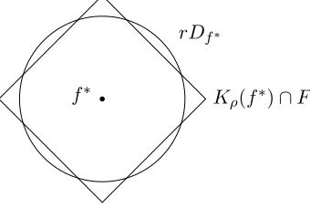
AS it happens, the geometry of the sets F∩Kρ(f∗) (see Figure1) determines both the error rate and the regularization parameter λ, while r(ρ) measures the sets’ ‘sizes’.
The choice of λis made as follows:
f∗ Kρ(f∗)∩F
rDf∗
Figure 1: Localization of the setF∩Kρ(f∗), i.e. its intersection withL2(µ)-balls of various radiir for the right choice of radiusρ, plays a central role in the analysis of the quadratic and multiplier processes.
Let
O(ρ) = sup|PNMf−f∗|:f ∈F∩Kρ(f∗)∩r(ρ)Df∗
and for τ >0 and 0< δ <1, set
γO(ρ, τ, δ) = inf{x >0 :P r(O(ρ)≤τ x)≥1−δ}
and
γO(ρ) =γO(ρ,3/(80η3), δ).
In other words,γO(ρ) is proportional to the smallest possible upper estimate onO(ρ) that still holds with probability at least 1−δ.
Definition 1.8 For any τ >0 and 0< δ <1, set
λ0(δ, τ) = sup ρ>0,f∗∈F
γO(ρ, τ, δ)
ρ .
To compare λ0(δ, τ) with rQ and rM, first note that rM(ρ) and O(ρ) both depend on
properties of the multiplier processes indexed by localizations ofF∩Kρ(f∗), and recall that
symmetrized and centered processes are essentially equivalent. Second, if r(ρ) = rM(ρ) thenγO(ρ)∼r2M(ρ); moreover,γO(ρ) is trivially bounded by∼r2(ρ) for the right choice of
τ and δ. However, ifrM(ρ)≤rQ(ρ), that is, whenr(ρ) =rQ(ρ) – which is the case whenρ
is very large – one may find that γO(ρ) is actually significantly smaller than ∼r2(ρ). This observation is of crucial importance because of the choice of the regularization parameter: for the right choice ofτ,γO(ρ)≤r2(ρ) and
λ0(δ, τ)≤ sup
ρ>0,f∗∈Fr
thus, one may be tempted to select the latter as a regularization term. However, there are natural examples in which supρ>0r2(ρ)/ρ = ∞, rendering that choice impossible, whereas supρ>0,f∗∈FγO(ρ)/ρ turns out to be finite. Of course, there are still cases in
which supρ>0,f∗∈Fr2(ρ)/ρis finite, andλ0(δ, τ) is of the same order as supρ>0,f∗∈FrM2 (ρ)/ρ,
though that is not the generic situation.
We now come to the main result of the article.
Theorem 1.9 Let F be a closed, convex class of functions that satisfies Assumption 1.2 with constantsκandε. SetΨ(·)to be a regularization function that satisfies Assumption1.1 with constant η. Furthermore, assume that limρ→0r(ρ) = 0 and put λ > λ0(δ,3/(80η3)).
If fˆis the RERM with a regularization parameter λas in (1.3), then with probability at least 1−2δ−2 exp(−N ε2/2),
kfˆ−f∗k2L2(µ)≤max n
r2 10ηΨ(f∗),
32
κ2ε
λΨ(f∗) o
. (1.14)
Observe that λ0 depends only on the oscillations of the multiplier process. Hence, if the
problem is noise-free then λ0 = 0, showing that any regularization parameter λ >0 would do. Moreover, in that case rM(ρ) = 0 and so one can choose r(ρ) ≥ rQ(ρ) obtaining an
error rate that depends only onr2
Q(10ηΨ(f∗)).
As noted previously, if one considers empirical risk minimization performed in F∗ = {f ∈ F : Ψ(f) ≤ Ψ(f∗)}, the resulting error rate is kf˜−f∗k2
L2(µ) ≤ c0r
2(cΨ(f∗)) for
a suitable absolute constant c0 and a constant c that depends on κ, ε and δ; moreover,
under some minor additional assumptions, that rate is optimal in the minimax sense (cf.
Lecu´e and Mendelson) when one takesr(ρ)∼maxrM(ρ), rQ(ρ) . Hence, up to constants
involved, the first term in Theorem1.9 is essentially the minimax rate that one can obtain if Ψ(f∗) were known.
If one chooses λ ∼ λ0(δ, τ) for τ = 3/(80η3) then the second term in (1.14) is of the
order of
λΨ(f∗) =sup
ρ,f∗
γO(ρ, τ, δ)
ρ
·Ψ(f∗).
Note that forρ that is of the order of Ψ(f∗), one has
γO(ρ, τ, δ)
ρ ·Ψ(f
∗)≤c
1γO(ρ, τ, δ)≤c2r2(c3Ψ(f∗)),
which coincides with the first term, up to the constants involved. Thus, the price that one has to pay for not knowing Ψ(f∗) is manifested in the need to take the supremum over all possible choices ofρ in the second term, rather than considering only the levelρ∼Ψ(f∗).
Thankfully, there are many natural cases in which that price is rather small, allowing for satisfactory outcomes of Theorem1.9 that are close to the minimax rate.
2. Proof of Theorem 1.9
of course, we will specify when a constant is absolute and when it depends on other pa-rameters). The values of these constants may change from line to line. The notationx∼y
(resp. x.y) means that there exist absolute constants 0< c < C for whichcy ≤x≤Cy
(resp. x ≤ Cy). If b > 0 is a parameter, then x .b y means that x ≤ C(b)y for some constantC(b) that depends only onb.
The normed space `dp is Rd endowed with the norm kxkp = Pj|xj|p
1/p
; the corre-sponding unit ball is denoted byBd
p and the unit Euclidean sphere inRd isSd−1.
Finally, from here on we writeP r andk kL2 without specifying the underlying measure.
The proof of Theorem1.9 follows an almost identical path as the proof of Theorem 3.2 from Lecu´e and Mendelson (to appear). The differences between the two arguments are minor and their source is the fact that unlikeLecu´e and Mendelson(to appear), here we do not assume that Ψ is a norm. In Remark2.2 we will outline how a version of Theorem1.9 may be derived directly from Theorem 3.2 in Lecu´e and Mendelson(to appear) when Ψ is a norm.
Theorem 1.9is an immediate outcome of the following lemma:
Lemma 2.1 Let λ0 = λ0(δ,3/(80η3)) and set λ > λ0. If limρ→0r(ρ) = 0, ρ ≥ 5ηΨ(f∗)
and ρ >0, then with probability at least 1−2δ−2 exp(−N ε2/2),
kfˆ−f∗k2L2 ≤maxr2(ρ),(32/(κ2ε))λΨ(f∗) .
To see how Lemma 2.1can be used to conclude the proof of Theorem 1.9, observe that if Ψ(f∗) > 0, one may simply select ρ = 5ηΨ(f∗) in the lemma. If, on the other hand, Ψ(f∗) = 0, let (γn)∞n=1 be a positive sequence decreasing to 0 and setAn={kfˆ−f∗kL2 ≤ γn}, which is a decreasing sequence of events. If P r(An) ≥1−ν for some 0≤ν ≤1 and
every nthen P r({fˆ=f∗}) ≥1−ν. Since limρ→0r(ρ) = 0, one may apply Lemma 2.1to
each member of a nonnegative sequenceρn that decreases to zero and for whichγn=r(ρn) decreases to zero. By Lemma2.1, P r(An) ≥1−2δ−2 exp(−N ε2/2) for everyn and the proof of Theorem 1.9follows.
Proof of Lemma 2.1. Fixf∗ and set ρ >0 that satisfiesρ≥5ηΨ(f∗). Let
F1 ={f ∈F : Ψ(f−f∗)≤ρ}=F∩Kρ(f∗),
and
F2 ={f ∈F : Ψ(f −f∗) =ρ}.
Clearly,F1is a convex set that containsf∗, and by the continuity of the real-valued function t → Ψ(f∗ +t(f −f∗)), every ray [f∗, f) that originates in f∗ and passes through some
f ∈F\F1 intersectsF2.
Let θ=κ2ε/16 and set
rQ(ρ) =rQ(F1, κε/32) and rM(ρ) =rM(F1, θ/5, δ/4).
There is an eventA0of probability at least 1−δ−2 exp(−N ε2/2), and for every (Xi, Yi)Ni=1∈
• Iff ∈F1 and kf−f∗kL2 ≥rQ(ρ) then
1
N N
X
i=1
(f−f∗)2(Xi)≥θkf −f∗k2L2.
• Iff ∈F1 then
1
N N
X
i=1
ξi(f −f∗)(Xi)−Eξ(f−f∗)(X)
≤ θ
4max{kf−f
∗k2
L2, rM2 (ρ)}.
In particular, if f ∈F1 and kf−f∗kL2 ≥r(ρ)≥max{rM(ρ), rQ(ρ)} then PNLf ≥
θ
2kf −f
∗k2 L2.
By the choice ofλ, there is an event A1 of probability at least 1−δ on which iff ∈F1 and
kf −f∗kL2 ≤r(ρ), then
2
N N
X
i=1
ξi(f−f∗)(Xi)−Eξ(f −f∗)(X)
< 3
80η3λρ <
3
5ηλρ. (2.1)
Set A=A0∩ A1 and let (Xi, Yi)Ni=1 ∈ A. The proof now follows in three steps:
(1) Show that the functionalf →PNLλf is bounded from below – away from zero – in F2.
(2) An outcome of (1) is that if f ∈F\F1,PNLλ
f >0; hence, ˆf 6∈F\F1.
(3) Finally, pin-point ˆf withinF1 ={f ∈F : Ψ(f −f∗)≤ρ}.
Step 1. Fixf ∈F2 and note that by the ‘triangle inequality’ satisfied by Ψ,
Ψ(f)≥η−1Ψ(f−f∗)−Ψ(f∗).
Recall that η−1Ψ(f −f∗)≥η−1ρ ≥5Ψ(f∗) and thus, Ψ(f)−Ψ(f∗) ≥(3/5)η−1ρ. Hence, ifkf −f∗kL2 ≥r(ρ) then
PNLλf ≥(θ/2)kf−f∗k2L2 +λρ·
3 5η >0.
On the other hand, by the choice of λ, ifkf−f∗kL2 ≤r(ρ) then
PNLλf ≥ −
1
N N
X
i=1
ξi(f −f∗)(Xi)−Eξ(f−f∗)(X)
+λ(Ψ(f)−Ψ(f∗))
≥ −
1
N N
X
i=1
ξi(f −f∗)(Xi)−Eξ(f−f∗)(X)
f∗
0
R > M R > M
R > M R > M
Q > M
Q > M Q > M
Q > M
f h
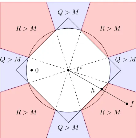
Figure 2: PNLλ
f >0 for two different reasons: either Q > M – the quadratic component
dominates the multiplier component, orR > M – the regularization component dominates the multiplier component. Unlike Theorem 3.2 inLecu´e and Mendelson
(to appear), here we chooseρ∼Ψ(f∗) to ensure that 0∈F ∩Kρ(f∗).
It should be noted that the same proof shows that on the event A, for everyf ∈F2, PNLf+
λ
2η2(Ψ(f)−Ψ(f
∗))>0, (2.2)
a fact that will be used below. Indeed, (λ/2η2)·(Ψ(f)−Ψ(f∗))≥(λ/2η2)·(3ρ/5η) and by (2.1), if kf−f∗kL2 ≤r(ρ) thenPNLf ≥ −(3/80)·(λρ/η3).
Step 2. Let f ∈ F\F1 and note that by the convexity of F and the continuity of Ψ on rays, there is some h∈F2 and R >1 for which f =f∗+R(h−f∗). Thus,
PNLλf = R
2 N
N
X
i=1
(h−f∗)2(Xi) +2R
N N
X
i=1
ξi(h−f∗)(Xi) +λ(Ψ(f)−Ψ(f∗)).
Observe that
Ψ(f)−Ψ(f∗)≥ R
2η2(Ψ(h)−Ψ(f
∗)) ; (2.3)
indeed,
Ψ(f∗+R(h−f∗))≥η−1Ψ(R(h−f∗))−Ψ(f∗)≥Rη−1Ψ(h−f∗)−Ψ(f∗),
and thus it suffices to show that
R
ηΨ(h−f ∗
)≥ R
2η2Ψ(h) + 2Ψ(f ∗
But since Ψ(h−f∗)≥5ηΨ(f∗),η ≥1 andR≥1, one has
R
ηΨ(h−f ∗
)≥ R
2ηΨ(h−f ∗
) +R
2Ψ(f
∗
) + 2RΨ(f∗)
≥R
2η (Ψ(h−f
∗) + Ψ(f∗)) + 2Ψ(f∗)≥ R
2η2Ψ(h) + 2Ψ(f ∗),
and (2.3) follows.
Finally, applying (2.2) toh∈F2,
PNLλf ≥R
2 N
N
X
i=1
(h−f∗)2(Xi) +2R
N N
X
i=1
ξi(h−f∗)(Xi) +λ R
2η2(Ψ(h)−Ψ(f ∗
))
≥R
PNLh+ λ
2η2(Ψ(h)−Ψ(f ∗
))
>0,
and ˆf 6∈F\F1.
Step 3. Turning toF1={f ∈F : Ψ(f−f∗)≤ρ}=F ∩Kρ(f∗), recall that if f ∈F1 and
kf −f∗kL2 ≥r(ρ), then PNLf ≥(θ/2)kf−f∗k2L2; hence, if f is a potential minimizer and
kf −f∗kL2 ≥r(ρ) then
0≥PNLλf ≥(θ/2)kf−f∗k2L2 +λ(Ψ(f)−Ψ(f∗))≥(θ/2)kf−f∗k2L2−λΨ(f∗),
and
kfˆ−f∗k2 L2 ≤
2λ θ Ψ(f
∗),
as claimed.
Remark 2.2 IfΨhappens to be a norm (which is an assumption slightly stronger than As-sumption 1.1), one may apply Theorem 3.2 from Lecu´e and Mendelson(to appear) directly. Indeed, and using the notation from Lecu´e and Mendelson (to appear) if ρ & Ψ(f∗) then the set K={f : Ψ(f−f∗)≤ρ/20} contains aΨ-ball around0, and Γf∗(ρ) – the collection
of norming functionals (i.e., the sub-gradient of Ψ) of any h ∈ K – is the entire unit ball in the dual space to (E,Ψ). Recall that
∆(ρ) = inf
h z∗∈Γfsup∗(ρ)
z∗(h−f∗),
where the infimum is taken in the set
{h∈F : Ψ(h−f∗) =ρ and kh−f∗kL2 ≤r(ρ)}.
3. Towards the examples - preliminary estimates
It is rather obvious that any implementation of Theorem 1.9 requires specific estimates on rM, rQ and λ0. This section is devoted to some preliminary facts that will play an
instrumental part in establishing such estimates.
Our main interest is the study of upper bounds on the three processes used to define the parameterrM,rQ andγO, and which have the following forms:
(∗) = sup
f∈F
N
X
i=1
εiξif(Xi)
, (∗∗) = sup
f∈F
N
X
i=1
(ξif(Xi)−Eξf(X))
and Esup
f∈F
N
X
i=1
εif(Xi) ,
where X1, ..., XN are independent and distributed according to the underlying measure µ,
ξ1, ..., ξN are independent copies of ξ ∈ Lq for some q > 2 (though (ξi)Ni=1 need not be
independent of (Xi)Ni=1), and (εi)Ni=1 are independent, symmetric {−1,1}-valued random
variables that are independent of (Xi)Ni=1 and (ξi)Ni=1.
Standard symmetrization methods (see, e.g., Gin´e and Zinn (1984); Ledoux and Tala-grand (1991); van der Vaart and Wellner(1996)) show that (∗) and (∗∗) are equivalent in expectation and in deviation (up to a slight restriction on the deviation parameter). We will present one example in which this symmetrization argument is carried out in full (Theorem 4.2), but in the other examples we will only consider the symmetrized case.
3.1 Estimates for subgaussian classes
The first result is fromMendelson(2016), under the assumption thatF is anL-subgaussian class of functions.
Definition 3.1 A class of functionsF ⊂L2(µ)isL-subgaussian if for everyf, h∈F∪ {0}
and every u≥1,
P r(|f(X)−h(X)| ≥Lukf−hkL2(µ))≤2 exp(−u2/2),
where X is distributed according toµ.
Let F ⊂ L2(µ) and set {Gf : f ∈ F} to be the centered, canonical Gaussian process
indexed byF (i.e., the covariance operator of the process isEGfGg =Ef(X)g(X) for every f, g∈F). Put
`∗(F) =Esup f∈F
Gf, and d2(F) = sup f∈F
kfkL2(µ). (3.1)
Theorem 3.2 (Corollary 1.10 in Mendelson (2016)) Let X be distributed according to µ, set ξ ∈ Lq for some q > 2 and assume that F ⊂ L2(µ) is an L-subgaussian class.
There are constants c, c0, c1, c2 and c3 that depend only on q, for which, for any w, u > c,
with probability at least
1− c0log
qN
wqNq/2−1 −2 exp −c1u
2(`∗(F)/d 2(F))2
sup
f∈F
1
N N
X
i=1
εiξif(Xi)
≤c2LwukξkLq `∗(F)
√
N
and
sup
f∈F
1
N N
X
i=1
ξif(Xi)−Eξf(X)
≤c2LwukξkLq `
∗(F)
√
N .
Corollary 3.3 Using the notation and assumptions of Theorem 3.2, let ξ = Y −f∗(X)
and assume thatξ ∈Lq for some q >2. Fix τ >0 and0< δ <1, and set A >0 for which
c2LwukξkLq`∗(F∩ADf∗)≤τ A2
√
N . (3.2)
If
δ ≥ c0log
qN
wqNq/2−1 + 2 exp −c1a0u 2
(3.3)
thenrM(F, τ, δ)≤A.
Proof. Clearly, it follows from Theorem 3.2that if
δ≥ c0log
qN
wqNq/2−1 + 2 exp −c1u 2
`∗(F∩ADf∗) d2(F ∩ADf∗)
2!
thenrM(F, τ, δ)≤A. The claim follows because if F∩ADf∗ is nonempty,
`∗(F ∩ADf∗) d2(F ∩ADf∗)
≥a0
for a suitable absolute constanta0.
Remark 3.4 The estimate in Corollary 3.3 can be rather loose. The reason for the sub-optimal estimate is that usually, the Gaussian mean-width `∗(F ∩ADf∗) is much larger
than d2(F ∩ADf∗). For example, let F = {t,· : t ∈ Sd−1} be the class of linear
func-tionals on Rd indexed by the Euclidean unit ball. Assume that X is an isotropic vector –
that is, its covariance structure coincides with the standard Euclidean structure on Rd; that f∗ = 0; and that A ≤ 1. Then F ∩ADf∗ = {t,· : ktk2 ≤ A}, d2(F ∩ADf∗) = A and `∗(F ∩ADf∗) =A
√
d, implying that
`∗(F ∩ADf∗) d2(F ∩ADf∗)
≥√d (3.4)
which is significantly larger than an absolute constant.
Having said that, the question of an accurate probability estimate is not the main issue of this article and we will not explore that point further.
Next, we provide an estimate on γO(ρ, τ, δ) that follows from Theorem 3.2 when F is
Corollary 3.5 Let F be a closed, convex L-subgaussian class of functions and let ξ =
Y −f∗(X) ∈ Lq for some q > 2. Set w, u > c, τ > 0, 0 < δ < 1 and ρ > 0. If A > 0
satisfies
c2LwukξkLq`
∗(F∩K
ρ(f∗)∩r(ρ)Df∗)≤τ A
√
N .
and
δ ≥ c0log
qN
wqNq/2−1 + 2 exp −c1a0u 2
thenγO(ρ, τ, δ)≤A.
Finally, whenF is anL-subgaussian class it follows from a standard chaining argument (cf. Talagrand (2005) or Mendelson (2016)) that
Esup f∈F
1
N N
X
i=1
εif(Xi) ≤
c0L`∗(F) √
N . (3.5)
This observation will be used in what follows to upper bound rQ.
3.2 Estimates under a limited moment condition
In this section we shall consider the case of a class that need not be subgaussian, but rather, the growth of moments of class members is well-behaved up to some point. More accurately, we will assume that there is somep0 for which, for every f, h∈F ∪ {0}and 2≤p≤p0,
kf −hkLp ≤L√pkf −hkL2. (3.6)
In contrast, a subgaussian condition is equivalent to havingkf−hkLp ≤L√pkf−hkL2 for everyp≥2.
The motivation behind this type of limited moment assumption is the LASSO estimator. Recent results on properties of the basis pursuit algorithm in Rd Lecu´e and Mendelson
(2017); Dirksen et al. (2014) indicate that the limited moment assumption (3.6) for p0 ∼ logd should suffice for an optimal estimate on the performance of the LASSO – as if the class were subgaussian.
When analyzing the LASSO via the computation of the fixed points rM and rQ, one
encounters the following scenario. Let X = (xj)dj=1 be a random vector in Rd and set X1, . . . , XN to be independent copies ofX. LetXi(j) be thej-th coordinate ofXiand thus
(Xi(j))Ni=1 is a random vector with independent coordinates, distributed asxj.
Consider the random variables appearing in the definition of rM and rQ in the LASSO case:
max
1≤j≤d
N
X
i=1
εiXi(j)
, (3.7)
and
max
1≤j≤d
N
X
i=1
εiξiXi(j)
The aim of this section is to derive upper bounds on (3.7) in expectation and (3.8) in deviation when each xj satisfies that
kxjkLp ≤L√pkxjkL2
forp.logd. Note that an upper bound on the centered empirical process involved in the definition ofγO(ρ) will follow from a symmetrization argument and a bound on (3.8).
The obvious difference between (3.7) and (3.8) are the multipliers (ξi)Ni=1: although the
xj’s have ∼logdmoments, ξ may be heavy-tailed, in the sense that it only belongs to Lq
for some fixed q >2; this difference makes the analysis of (3.8) more difficult. Upper bounds on (3.7) and (3.8) are obtained under the following assumption.
Assumption 3.1 Let N ≤d, t ≥4 and set p0 = tlogd. Assume that p0 .N (and note that p0 ≥logN) and that for every1≤j≤d and p≤p0, kxjkLp ≤L√pkxjkL2. Consider
ξ∈Lq for someq >2; let r= min{1/2 +q/4,2}; set r0 to be the conjugate index ofr; and
assume that4r0max{2,1 +a0/a1} ≤tlogN (where a0 anda1 are two absolute constants to be specified later – in Lemma 7.3 and Lemma7.4).
Under this assumption we will prove the following:
Theorem 3.6 Let the random vectorX andξ =Y−f∗(X) satisfy Assumption3.1. Then,
E max 1≤i≤d
1 √
N N
X
i=1
εiXi(j)
≤c0plogd·L max
1≤j≤dkxjkL2. (3.9)
Also, for every u > 2, v >0, w ≥2 and forp =p0/2 and m =p/log(eN/p), one has that with probability at least
1−exp(−p/2)
u2p −
4 exp(−p/2)
uc1m −
c2logqN
wqNq/2−1 −2 exp(−v
2tlogd), (3.10)
max
1≤j≤d
N
X
i=1
εiξiXi(j)
≤c3(q)(uw+u
2v)Lkξk Lq
√
Nptlogd max
1≤j≤dkxjkL2. (3.11)
The proofs of both estimates in Theorem 3.6 follow from a more general result, es-tablished in Mendelson (2016), on the supremum of a centered multiplier process under a limited moment assumption like (3.6). Although the estimate inMendelson(2016) is stated for the centered empirical process (cf. Section 4 there) its proof is actually based on an estimate on the symmetrized process. The proof of Theorem3.6will be presented in a final section of this article.
4. The LASSO under a limited moment assumption
The rate we shall be comparing the LASSO’s performance to is the minimax rate of the following problem. Let X∼ N(0, Id×d) and set ξ ∼ N(0, σ2) to be independent of X. Let
ρ >0, consider an unknown t0 ∈ρB1dand put Y =
X, t0
+ξ.
Let c0, c1 and c2 be well-chosen absolute constants and consider the cases logd≤N ≤ c0dorc1d≤N. FollowingLecu´e and Mendelson, if
s2M(ρ) =c2
σ2d
N ifρ
2N ≥σ2d2 ρσ
r
1 N log
eσd ρ√N
ifσ2logd≤ρ2N ≤σ2d2 ρσ
q
logd
N ifρ
2N ≤σ2logd
and s2Q(ρ)
= 0 ifN ≥c0d
.ρ2/d ifc0d≤N ≤c1d
∼ ρN2 logNd ifN ≤c1d,
then the minimax rate of convergence in the class ρBd1 is
maxns2M(ρ), s2Q(ρ)o (4.1)
when ρ ≥ σp(logd)/N and ρ2 when ρ ≤ σp(logd)/N. Note that when c0d ≤N ≤ c1d
(i.e. N ∼d),s2Q(ρ) decays rapidly from ρN2log(d/N) to 0 and there are no precise estimates on the minimax rate in that range.
It turns out that for this problem – the so-called Gaussian linear model – the minimax rate inρBd
1 is achieved by the Empirical Risk Minimization procedure (see, e.g.,Lecu´e and Mendelson); however, an underlying assumption is thatρis given. Thanks to regularization, and specifically, thanks to the LASSO, one does not need to know the value of kt0k1 in
advance to achieve the minimax rate, at least up to a logarithmic term. In fact, as will be explained below, the optimal rate can be achieved using regularization in a much more general framework than just the Gaussian linear model.
In what follows we focus on the performance of the LASSO in the high-dimensional case, that is, whenN ≤c1d. One may do the same whenN ≥c0dand we leave that to the reader.
Let X be a random vector in Rd and consider the class of linear functionals F ={ft=
·, t : t ∈ Rd}. In particular, if Y ∈ L2 is an arbitrary target random variable then f∗=ft∗ =·, t∗satisfies
t∗ ∈argmin
t∈Rd
E Y −X, t2. (4.2)
As noted in the introduction, the regularization function associated with the LASSO is the
`d1-norm: for every t= (tj)dj=1∈Rd,
Ψ(ft) =ktk1=
d
X
j=1
|tj|.
Clearly, as a norm, the`d
1-regularization function satisfies Assumption 1.1forη= 1.
The LASSO with regularization parameter λproduces
ˆ
t∈argmin
t∈Rd
1
N N
X
i=1
Yi−
and one would like to control kfˆt−ft∗k2L2 =E
X,ˆt−t∗2, where the expectation is taken with respect toX conditionally on the data.
It should be noted that despite the LASSO’s popularity, there are relatively few results in the random design scenario we are interested in (see, e.g.,Bartlett et al.(2012),Massart and Meynet (2011) and chapter 8.2 in Koltchinskii (2011)). The overwhelming majority of existing results have been obtained for the linear model with subgaussian noise and a fixed design (i.e., each data point is of the form Yi =
t∗, zi
+ξi), and the deterministic
design matrix, whose rows are the vectors zi, which satisfies some form of the restricted
isometry property – for example, the Restricted Eigenvalue Condition (REC) from Bickel et al. (2009) or theCompatibility Condition (CC) from van de Geer(2007)).
To define the restricted eigenvalue condition, let us introduce the following notation: for
x∈Rd and a set S
0 ⊂ {1, . . . , d} of cardinality |S0| ≤s, letS1 be the set of indices of the m largest coordinates of (|xi|)di=1 that are outside S0. Let xS01 be the restriction of x to
the set S01=S0∪S1.
Definition 4.1 (Bickel et al. (2009)) Let Γ be an N×d matrix. For c0 ≥ 1 and an
integer 1≤s≤m≤dfor which m+s≤d, the restricted eigenvalue constantis
κ(s, m, c0) = min
kΓ
xk2
kxS01k2 :S0⊂ {1, . . . , d},|S0| ≤s, xSc
0
1≤c0kxS0k1
.
The matrix Γ satisfies the Restricted Eigenvalue Condition (REC) of order s with a constant c if κ(s, s,3)≥c.
One can show (see, Bickel et al. (2009), B¨uhlmann and van de Geer (2011)) that if Γ satisfies REC andλ&σp(logd)/N, then with high probability (with respect to the noise), simultaneously for every 1≤p≤2,
tˆ−t∗
p p .pkt
∗k 0
σ κ(s, s,3)
r logd
N
!p
(4.4)
wherekt∗k0 is the cardinality of the support of t∗.
The main result in this section is an estimate on kfˆ−f∗k2
L2 that depends on kt∗k1
rather than on the cardinality of the support of t∗ (we refer to Lecu´e and Mendelson (to appear) for sparsity-dependent rates of convergence for the LASSO in the same framework as we consider here). Such a result follows from Theorem 1.9, and to that end, one has to construct a functionr(·) as in (1.13) and to computeλ0(δ, γ) as in Definition1.8. We will do
so in the following case: Seta2≥4, 2≤p0 =a2logd.N,q >2,r= min{1/2+q/4,2}and
r0 that is the conjugate index of r. Assume that 4r0max{2,1 +a0/a1} ≤ a2logN (which
is equivalent to assuming that q > 2 +c1/logN for some constant c1 = c1(a0, a1, a2)).
Let X = (xj)dj=1 be a random vector and note that the coordinates x1, ..., xd need not be independent.
Assumption 4.1 Using the above notation, assume that there are constants κ0, κ and ε
• For every 1≤j≤dand every 2≤p≤p0, kxjkLp ≤κ0
√
pkxjkL2.
• X satisfies a small-ball condition with constants κ and ε; that is, for every t∈Rd,
P r
|
X, t| ≥κ
X, t
L2
≥ε. (4.5)
• ξ =Y −f∗(X)∈Lq.
To put this assumption in some perspective, note that an obvious underlying condition in any estimation problem with respect to the squared loss is that E(f(X)−Y)2 is defined
for any f ∈ F, and in particular, that ξ =Y −f∗(X) ∈ L2. Thus, assuming that ξ ∈Lq
for some q >2 +c1/logN is not very restrictive. Also, as noted previously, the small-ball assumption is rather minimal.
The most restrictive component of Assumption 4.1 is the moment assumption on the
coordinates ofX, namely that their moments exhibit a subgaussian behavior, up to, roughly,
p∼logd.
While this assumption can be weakened to other types of moment growth condition (e.g., kxjkLp≤κ0pαkxjkL2 for some α≥1/2 and up top∼logd), the resulting analysis is more involved (see Lecu´e and Mendelson(2017)), and will not be explored here.
Finally, Lecu´e and Mendelson (2017) shows that even if one assumes a subgaussian behavior of the coordinatesxi, but only up top∼(logd)/(log logd), Basis Pursuit may fail
to recover even a 1-sparse vector, implying that the choice ofp0 in Assumption 4.1can not
be relaxed significantly.
Given any ρ≥0, set M = max1≤j≤dkxjkL2, let σq =kξkq and put
Λ(ρ) = κ0ρM
κ2ε
r logd
N .
Moreover, for R(t) =E(Y −X, t)2, one has
R(t)−R(t∗) =EX, t−t∗2,
because X, t∗ is the best approximation of Y in a closed subspace of L2. Thus, the estimation bounds also lead to excess risk bounds.
Theorem 4.2 There are absolute constantsc0, ..., c6 for which the following holds. Assume
that X and ξ =Y −f∗(X) satisfy Assumption 4.1 and that N ≤d. Let u >2, v >0 and
w≥2, and set p= (a2/2) logdand m=p/log(eN/p). Put
δ = exp(−p/2)
u2p −
4 exp(−p/2)
uc0m −
c1logqN
wqNq/2−1 −2 exp(−v
2tlogd) (4.6)
and set
r2(ρ) =c2
(
(uw+u2w)σqΛ(ρ) if N ≥(κε/32)2d
max n
(uw+u2v)σqΛ(ρ), κ2Λ2(ρ) o
If ˆt is produced by the LASSO for a regularization parameter
λ > c4(uw+u2v)κ0kξkLqη3M
r logd
N ,
then with probability at least 1−5δ−2 exp(−ε2N/2),
R(ˆt)−R(t∗) =
X,ˆt−t∗
2
L2 ≤c5max
n
r2(c6kt∗k1), λ κ2εkt
∗k 1
o
.
Observe that like known estimates on the LASSO, and despite imposing considerably weaker assumptions on X and Y, the regularization parameter in Theorem 4.2 is of the order of kξkLqp
(logd)/N. And, when kξkLq is equivalent to σ – theL2 norm of ξ – then
forN .d, the rate of convergence is
c(M) max (
σkt∗k1 r
logd N ,kt
∗k2 1
logd N
)
for a constant c(M) that depends only onM.
Hence, up to a logarithmic factor, the LASSO attains the minimax rate in kt∗k1B1d
when logd≤N .dand when kt∗k1 ≥σplogd/N; moreover, it does so without knowing in advance the identity of the true modelkt∗k1Bd1.
Note that one may want to combine the sparsity-dependent error rate from Theorem 1.3 in Lecu´e and Mendelson (to appear) and the complexity-dependent error rate from Theo-rem 4.2. To simplify the formulation we assume that X is subgaussian, in which case the probability estimate in Theorem 4.2 can be improved and the third condition in Assump-tion 4.1 (i.e. that q > 2 +c1/logN) can be relaxed to only q > 2 (see more details in the next section, and, in particular, Theorem5.4). Combining the two approaches, one has that whenX is isotropic andL-subgaussian, and when ξ ∈Lq for someq >2 then for any u, w > cwith probability larger than 1−δ for
δ = 2 exp(−c2N/L8)−
c0logqN
wqNq/2−1 −c0exp(−c1u 2/L2),
the LASSO estimator ˆt with the universal regularization parameter kξkLqp
(logd)/N sat-isfies that
ˆt−t∗
2
2 .L,qmin
(
kt∗k0σ2logd
N ,max
(
σkt∗k1 r
logd N ,kt
∗k2 1
logd N
))
(4.7)
when N &kt∗k0log(d/kt∗k0).
Observe that (4.7) seemingly exhibits a different rate than Corollary 9.1 inKoltchinskii
(2011) (see also (1.4)), the difference being the extra (and necessary)kt∗k21 logNd term in (4.7). This extra term appears only in the random design scenario, and the rates of convergence of the LASSO appear to deteriorate when
σ
s
N
logd ≤ kt ∗k
1≤σ
q kt∗k
However, the sparsity-dependent error rate, and therefore Equation (4.7), holds only when
N & kt∗k0log(d/kt∗k0). And, when N & kt∗k0logd (which is only slightly larger than kt∗k0log(d/kt∗k0)), the error rates in the two scenarii (random and deterministic design) are the same and are given by
min (
σ2kt∗k0logd
N , σkt
∗k 1 r logd N ) .
Proof of Theorem 4.2. As noted previously, since k·k1 is a norm, Ψ(t) = ktk1 satisfies
Assumption 1.1 for η = 1 and Theorem 1.9 may be applied. To that end, one has to
control r(ρ) ≡max{rM(ρ), rQ(ρ)} and λ0(δ, τ). In what follows we will invoke the results of Section 3 and estimate these parameters.
Set F(f∗, ρ) = F ∩Kρ(f∗)−f∗ and recall that rQ(ρ) = rQ(F ∩Kρ(f∗), κε/32) is determined by the behavior of
(?) =E sup
f∈F(f∗,ρ)∩rD
1 √ N N X i=1
εif(Xi)
; (4.9)
as a consequence, it suffices to upper bound (?). Let E ={t ∈Rd:
EX, t2 ≤1}, put E◦
to be the polar of E (that is, E◦ ={u : sup t∈E|
u, t
| ≤ 1}), and set ktkE = supx∈E
x, t . Thus,
(?) =E sup t∈ρBd 1∩rE 1 √ N N X i=1
εiXi, t
≤min ( E sup t∈ρBd 1 1 √ N N X i=1
εiXi, t
,Esup t∈rE 1 √ N N X i=1
εiXi, t
) = min ρE 1 √ N N X i=1 εiXi
`d ∞
, rE
1 √ N N X i=1 εiXi
E◦ .
It is standard to verify (see, for instance, the proof of Lemma 2.2 inLecu´e and Mendelson
(2016)) that
E 1 √ N N X i=1 εiXi
E◦
≤√d.
Moreover, by (3.9),
E 1 √ N N X i=1 εiXi
`d ∞
=E max
1≤j≤d 1 √ N N X i=1
εiXi(j)
≤c0κ0
p
logd max
1≤j≤dkxjkL2.
Therefore,
(?)≤min
c0ρκ0plogd max
1≤j≤dkxjkL2, r
√
d
and setting γ=κε/32, one has
rQ(ρ)≤ (
0 ifN ≥γ2d
c0ρκ0 γ
q
logd
N M otherwise.
Next, let us establish a high probability upper bound onrM(ρ) =rM(F∩Kρ(f∗), κ2ε/80, δ/4). Note that
φN(F∩Kρ(f∗), f∗, s) = sup t∈ρBd 1∩sE 1 √ N N X i=1 εiξi
Xi, t
≤ρ max
1≤j≤d 1 √ N N X i=1
εiξiXi(j)
.
Applying the second part of Theorem 3.6 for u > 2, v > 0, w ≥ 2, p = (a2/2) logd, m = p/log(eN/p) and
δ = exp(−p/2)
u2p −
4 exp(−p/2)
uc0m −
c1logqN
wqNq/2−1 −2 exp(−v
2tlogd), (4.11)
it follows that with probability at least 1−δ,
φN(F ∩Kρ(f∗), f∗, s)≤c2κ0(uw+u2v)kξkLqρM
p logd;
thus,
rM2 (ρ)≤ c3κ0(uw+u
2v)
κ2ε kξkLqρM
r logd
N .
Finally, let us identify an upper bound on λ0(δ, τ) forτ = 3/(80η3). Let{e1, . . . , ed}be
the canonical basis of Rd. SinceKρ(f∗) ={t:kt−t∗k1 ≤ρ}, we have
(?1) = sup
f∈F∩Kρ(f∗)∩r(ρ)D f∗ 1 N N X i=1
ξi(f −f∗)(Xi)−Eξ(f−f∗)(X)
!
≤ρ max
t−t∗∈{±e1,...,±ed}
1 N N X i=1 ξi
Xi, t−t∗
−EξX, t−t∗
!
=ρ max
t∈{±e1,...,±ed} 1 N N X i=1
ξiXi, t−EξX, t
!
.
Recall that X = (xj)dj=1. By a standard symmetrization argument (see, for example,
Lemma 2.3.7 in van der Vaart and Wellner(1996)), ifz≥4 max1≤j≤d
p
Var(ξxj)/N then
P r max
t∈{±e1,...,±ed}
1 N N X i=1 ξi
Xi, t
−Eξ
X, t
≥z≤4P r max
t∈{±e1,...,±ed} 1 N N X i=1 εiξi
Xi, t
≥ z
4
.
Note that pVar(ξxj) ≤qEξ2xj2 ≤ kξkLqkxjkL2q0 where q
0 is the conjugate index of q/2.
Therefore, pVar(ξxj) ≤ κ0√2q0kξk
LqM as long as 2q
2/(a2logd−1) – which is the case under Assumption 4.1. Therefore, applying the second
part of Theorem3.6 forδ as in (4.11), it follows that with probability at least 1−δ,
(?1)≤ρc0κ0(uw+u2v)kξkLqM
r logd
N ,
and, forτ = 3/(80η3) one may select
λ0(δ, τ) =c4κ0(uw+u2v)kξkLqη3wM
r logd
N .
5. Regularization methods for subgaussian classes
In this section, we assume thatXis a random vector that takes its values in a Hilbert space H. The main examples we consider are when H is thed-dimensional Euclidean space and when it is the space ofm×T matrices endowed with the Frobenius norm.
The inner product inHis denoted by·,·
, and the norm and unit ball endowed by the inner product are denoted byk·kH and BH={t∈ H:ktkH≤1} respectively.
There is another natural Hilbertian structure on H, endowed by Σ = EXX>, the
covariance operator associated with the random vector X. The corresponding unit ball E ={t∈ H:EX, t2 ≤1}, is an ellipsoid inH.
Let T ⊂ H be a closed and convex set and put
t∗∈argmin
t∈T E
(Y −
X, t)2.
Let Ψ(·) be a regularization function on Hthat satisfies Assumption1.1 and set
ˆ
t∈argmin
t∈T
1
N N
X
i=1 Yi−
Xi, t
2
+λΨ(t) (5.1)
for a well-chosen regularization parameterλ.
Unlike the results of the previous section, in what follows we assume that F ={
t,· :
t ∈ T} is an L-subgaussian class (see Definition 3.1). Moreover, F satisfies a small-ball property with constants that depend only on L. Indeed, observe that for everyt∈T
X, t
L4 .L
X, t
L2,
and applying the Paley-Zygmund inequality (see, e.g., Corollary 3.3.2 in de la Pe˜na and Gin´e (1999)),
P r
|
X, t| ≥κ
X, t
L2
≥εforκ= 1/2 andε=c/L4. (5.2)
From here on we say that the random vectorXtaking its values inHisL-subgaussian if the class consisting of all the linear functionals onH, i.e.,{
t,·
:t∈ H}, isL-subgaussian. Also, throughout this section, we assume that ξ = Y −f∗(X) ∈ Lq for some q > 2, and
denote σq=kξkLq and
5.1 ‘Heavy tailed’ noise
Thanks to the subgaussian assumption, both r(ρ) and λ0 =λ0(δ,3/(80η3)) may be deter-mined using the Gaussian mean-widths of the sets T ∩Kρ(t∗) for all ρ > 0. Recall that
for T0 ⊂ H the Gaussian mean-width of T0 is `∗(T0) = Esupt∈T0Gt, where (Gt)t∈T0 is
the centered canonical Gaussian process indexed by T0 with covariance structure given by
EGt1Gt2 =EX, t1
X, t2
for every t1, t2∈T.
Definition 5.1 Let rEt∗ =t∈ H:kt−t∗,·kL2(µ)≤r =t∗+rE, and for α, β >0 set
˜
rQ(ρ, α) = inf n
r >0 :`∗(T∩Kρ(t∗)∩rEt∗)≤αr
√
N
o
and
˜
rM(ρ, β) = inf
n
r >0 :`∗(T ∩Kρ(t∗)∩rEt∗)≤βr2
√
No.
Let c0 be an absolute constant to be specified later. Fix u, w > c, and ε and κ as in (5.2). Consider
α= κε
c0L
, β= κ
2c 1ε
LwukξkLq, and γ =c0η
3Lwukξk
Lq, (5.3)
put
r(ρ)≥max{˜rQ(ρ, α),r˜M(ρ, β)} (5.4)
and set
λ0(γ) =γ sup
ρ>0,t∗∈T
`∗(T∩Kρ(t∗)∩r(ρ)Et∗)
ρ√N . (5.5)
The first result we present is rather general and holds for any closed and convex subset
T ⊂ H and any regularization function satisfying Assumption 1.1. It allows one to take into account an additional constraint on the “signal”t∗ ∈T.
Theorem 5.2 There are absolute constants c, c1 and c2 for which the following holds. Let
Ψbe a regularization function satisfying Assumption 1.1. Assume that X isL-subgaussian for some L >0 and that ξ =Y −
X, t∗
is inLq for some q >2.
If ˆt is given by (5.1) for a regularization parameter λ > λ0(γ) as in (5.5), then with
probability larger than
1−2 exp(−N ε2/8)− c0log
qN
wqNq/2−1 −c0exp(−c1u
2/L2), (5.6)
X,tˆ−t∗
2
L2 ≤max
r(10ηΨ(t∗))2,(32/κ2ε)λΨ(t∗)
for r(·) given by (5.4).
Since X is L-subgaussian, the process
X, t
:t∈ H is L-subgaussian. Setting F = {
t,·
:t∈ H} andf∗ =t∗,·
, a standard chaining argument shows that
E sup
f∈F∩Kρ(f∗)∩rD f∗
1
N N
X
i=1
εi(f−f∗)(Xi)
≤c0L
`∗(T∩Kρ(t∗)∩rEt∗)
√
N .
Thus,
rQ
F∩Kρ(f∗), κε
32
≤˜rQ(ρ, α). (5.7)
As for the fixed point associated with the multiplier process, it follows from Corollary3.3 that
rM
F∩Kρ(f∗),κ 2ε
160,
δ
4
≤r˜M(ρ, β) (5.8)
forβ as defined in (5.3), and as long as
δ
4 ≥
c0logqN
wqNq/2−1 + 2 exp(−c1u 2/L2).
Finally by Corollary 3.5,λ0(δ, γ)≤λ0(γ). The claim now follows from Theorem1.9.
If one is to apply Theorem 5.2, an essential component is an upper bound on `∗(T ∩
Kρ(t∗)∩rEt∗), leading to estimates on r and λ. To simplify the analysis we shall use an
additional assumption on Ψ:
Assumption 5.1 Assume that for every x, y∈ H andλ≥0,
Ψ(x) = Ψ(−x), Ψ(x+y)≤η Ψ(x) + Ψ(y) and Ψ(λx)≤λΨ(x). (5.9)
Also, recall that E={t∈ H:EX, t2≤1},σq =kξkq and setK ={t∈ H: Ψ(t)≤1}. Theorem 5.3 Assume thatΨ satisfies Assumption 5.1and that the assumptions of Theo-rem 5.2hold. Let Λ(ρ)≥ρ`∗(K)/√N for everyρ >0,w, u > c and consider the RERM
ˆ
t∈argmin
t∈H
1
N N
X
i=1
(Yi−
Xi, t)2+c0η3LwuσqΛ(Ψ(t))
.
Then, with probability larger than the one in (5.6),
R(ˆt)−R(t∗) =
X,tˆ−t∗
2
L2 ≤c0r
2(10ηΨ(t∗))
where, forα and β defined in (5.3) and, for any ρ≥0,
r2(ρ) =
( Λ(ρ)
β if N ≥ `
∗(E)/α2 maxnΛ(ρ)β ,Λ2α(ρ)2
o
otherwise. (5.10)
Proof. The result follows immediately from Theorem 5.2. Indeed, for every ρ >0, r >0 and t∗∈T =H,
`∗(T ∩Kρ(t∗)∩rEt∗) =`∗(Kρ(0)∩rE)≤`∗(ρK∩rE)≤min{ρ`∗(K), r`∗(E)},
Note that in a d-dimensional space, the trivial bound `∗(E) ≤ √d holds (see, e.g., Lemma 2.2 in Lecu´e and Mendelson (2016)). Therefore, one only needs to control `∗(K). In the next section, we provide several examples of applications of Theorem5.3that follow from estimates on `∗(K). We will simplify the analysis further by assuming that there is some compatibility between the normk·kHand the one endowed by the covariance structure of X:
Assumption 5.2 Assume that X is isotropic; that is, for every t ∈ H, EX, t21/2 =
ktkH.
Observe that Assumption 5.2 implies that `∗(K) = Esupt∈KGt, where (Gt)t∈K is the
canonical Gaussian process indexed by K with the covariance EGt1Gt2 =t1, t2for every t1, t2 ∈ K. Indeed, this follows because the inner-product in H coincides with the one
endowed byL2(µ).
5.2 Regularization methods in Rd
Consider a regularization function Ψ(·) satisfying Assumption 5.1. Assume that X is L -subgaussian and isotropic inRd with respect to the standard Euclidean inner-product, and
thatξ ∈Lq for someq >2. Letu, w > c. For anyρ≥0 set Λ(ρ)≥ρ`∗(K)/
√
N and put
r2(ρ)∼L,q
wuσqΛ(ρ) when N &Ld
maxwuσqΛ(ρ),Λ2(ρ) otherwise. It follows from Theorem5.3 that if
ˆ
t∈argmin
t∈Rd
1
N N
X
i=1
(Yi−
Xi, t
)2+c0η3LwuσqΛ(Ψ(t))
(5.11)
then with probability larger than the one in (5.6)
ˆ
t−t∗,·
2
L2(µ) .r
2(10ηΨ(t∗)).
As a consequence, one can derive an estimation result for (5.11) whenever `∗(K) may be controlled from above. In the following section, we shall apply this observation to some classical problems and compare the error rates obtained by the RERM (5.11) to the minimax rate in the true model{t∈T : Ψ(t)≤Ψ(t∗)}.
Example: `p-regularization for 1 ≤ p ≤ ∞. Consider the regularization function
Ψ(t) = ktkp for some p ≥1. Assumption 5.1 holds with η = 1 because k·kp is a norm. In order to apply the general result for the RERM in (5.11), one has to estimate the Gaussian mean-width of the unit ball associated with the regularization function Ψ(·) =k·kp.
In the range 1 ≤ p ≤ 1 + (logd)−1, we obtain the same performance as the LASSO, becauseBd1 ⊂Bpd⊂cB1dfor a suitable absolute constantc, implying that`∗(Bpd)∼`∗(B1d)∼ p
log(ed).
When 1 + (log(ed))−1 ≤ p, set r to be the conjugate index for p and one may easily verify that `∗(Bdp)∼√rd1/r.
Theorem 5.4 Under the assumptions of Theorem 5.3 and using its notation,
• If 1≤p≤1 + 1/(logd) and
ˆ
t∈argmin
t∈Rd
1
N N
X
i=1
(Yi−
Xi, t
)2+c2ηp3Lwuσqktkp
r logd
N
then with probability larger than the one in (5.6),
ˆt−t∗
2 2.p,L,q
wuσqkt∗kp q
logd
N if N &Ld,
max
wuσqkt∗kp q
logd N ,kt
∗k2 p
logd N
otherwise.
• If p≥1 + 1/(logd) and
ˆ
t∈argmin
t∈Rd
1
N N
X
i=1
(Yi−
Xi, t
)2+c2σqLwuktkp
p
p/(p−1)d(p−1)/p
√
N
,
then with probability larger than the one in (5.6)
ˆt−t∗
2 2 .L,q
wuσqkt∗kp d (p−1)/p
p√N if N &Ld,
max n
wuσqkt∗kp d(p√−1)/p N ,kt
∗k2 p
d2(p−1)/p N
o
otherwise.
Remark. [the case 0 < p < 1] Despite being a non-convex function, `p-regularization
for 0< p < 1 has attracted much attention in the context of Signal Processing and High-Dimensional Statistics. Among the problems studied using`pregularization were the linear
regression model with a deterministic design (cf. Raskutti et al.(2011); Rigollet and Tsy-bakov (2011); Verzelen (2012)); the sequence space model Donoho and Johnstone (1994);
Abramovich et al.(2006); and the random design linear regression modelWang et al.(2014). From our point of view, there is no particular restriction onpas long as the regularization function satisfies Assumption 5.1. We can therefore consider the regularization function Ψ(t) =ktkp for any 0< p < 1. In that range ofp, Assumption 5.1 holds forη =ηp = 21/p
(see, for example, page 2 inEdmunds and Triebel(1996)) and the Gaussian mean width of the “unit ball” associated with Ψ(·) =k·kp for 0< p <1 can also be computed.
To that end, let{e1, . . . , ed}be the canonical basis of Rd. Since{±e1, . . . ,±ed} ⊂Bdp ⊂ B1d forp <1, it is evident that`∗(Bpd)∼√logd. Thus, the error rates of the LASSO from Theorem4.2 dominate all the`p-regularization rates when 0< p≤1.
However, the resulting rate is not the minimax rate in the true model, as can be seen from Raskutti et al. (2011). Indeed, fix 0 < p ≤ 1. Consider an unknown t∗ ∈ ρBpd
and the corresponding Gaussian linear model Yi =
xi, t∗
+Wi, i = 1, . . . , N, where the