AUT J. Model. Simul., 50(2) (2018) 109-116 DOI: 10.22060/miscj.2017.12143.5005
Adaptive Tuning of Model Predictive Control Parameters Based on Analytical Results
T. Gholaminejad1*, A. Khaki-Sedigh1, P. Bagheri21 Department of Electrical Engineering, K. N. Toosi University of Technology, Tehran, Iran
2 Control Engineering Department Faculty of Electrical and Computer Engineering, University of Tabriz, Tabriz, Iran
ABSTRACT: In dealing with model predictive controllers (MPC), controller tuning is a key designing step. Various tuning methods are proposed in the literature which can be categorized as heuristic, numerical and analytical methods. Among the available tuning methods, analytical approaches are more interesting and useful. This paper is based on a proposed analytical MPC tuning approach for plants which can be approximated by first-order plus dead-time models. The performance of such methods fails to deal with unknown or time-varying parameter plants. To overcome this problem, adaptive MPC tuning strategies are practical alternatives. The adaptive MPC tuning approach proposed in this paper is based on on-line identification and analytical tuning formulas. Simulation results are used to show the effectiveness of the proposed methodology. Also, a comparison of the proposed adaptive tuning method with a well-known online tuning method is presented briefly which shows the superiority of the proposed adaptive tuning method.
Review History:
Received: 10 November 2016 Revised: 2 June 2017 Accepted: 11 June 2017 Available Online: 16 June 2017
Keywords:
Adaptive model predictive control analytical tuning
first order plus dead time models
1- Introduction
Model Predictive Control (MPC) is a well-established control technique used in advanced process control systems. Successful applications of MPC have been reported in many papers [1, 2]. MPC has several tuning parameters that must be appropriately tuned for acceptable closed-loop performances. Conventional tuning parameters of MPC are the prediction and control horizons and the weighted matrices. These parameters can significantly influence both the closed-loop performance and stability characteristics and therefore have been extensively studied in many research papers [3]. For example, Dynamic Matrix Control (DMC) tuning equations are developed in [4, 5] based on the analysis of variance. There is a tendency for closed-form tuning equations based on analytical methods, since they can be easily implemented and are also useful in the closed-loop analysis. In [6], an analytical MPC tuning approach is presented. Considering First Order Plus Dead Time (FOPDT) model of the real system, the closed-loop transfer function is derived, and it is shown that the maximum achievable performance can be obtained by the control horizon of one and two. Also, this approach is extended to unstable plants with the fractional delay [7] and multivariable plants [8]. However, these methods are inappropriate for unknown or time-varying plants. Adaptive tuning algorithms are suitable for these cases. In [9], an intuitive on-line MPC tuning strategy is presented, where a linear approximation between the output predictions and the MPC tuning parameters is utilized. In this set-up, the predicted outputs and the weights on the predicted outputs error and control action are related by sensitivity expressions which have been employed for automatic online adjustments of the parameters. In [9], a fuzzy logic-based auto-tuning strategy is provided for model predictive controllers, and in
[15] a similar strategy is suggested for non-linear MPC. In [16], a numerical auto-tuning algorithm is developed for DMC without constraint considerations. In this approach, Genetic Algorithm (GA) and Multi-Objective Fuzzy Decision-Making (MOFDM) strategies are combined to determine the optimal tuning parameters, where an objective function is calculated for each tuning parameter set. Then, based on the MOFDM algorithm, the best two sets of tuning parameters enter the next GA iteration while the worst set is eliminated. At the end of the GA cycle, the optimal tuning parameters are selected. In [17], it was proposed to auto-tune the GPC based on the characteristics of a second-order process such as rise time, settling time and overshoot. In this scheme, the auto-tuned GPC was used in a programmable logic controller. Finally, [14] proposed an MPC auto-tuning method to achieve the minimum variance output. This requirement is performed by forcing the MPC system to track its optimal closed-loop bandwidth. In this paper, an adaptive tuning algorithm for MPC based on the results of [6] is developed. It is shown that the proposed method can be used for all “unknown”, “time-varying”, “stable” systems with arbitrary order which can be approximated by an FOPDT model in an acceptable approximation. Note that many industrial processes can be sufficiently described by FOPDT models [18]. Also note that it is supposed that the variation of the systems is such that the robust control rules are not efficient.
The present paper is organized as follows. The MPC formulation and the tuning strategy given by [6] are briefly introduced in section II. A short study of the Recursive Least Square (RLS) method is provided in section III. Then, the proposed adaptive MPC tuning algorithm is developed and tested via simulation examples. Then, a comparison of the proposed adaptive tuning method with a well-known online tuning method is presented briefly. Finally, the conclusion of the paper is given.
2- Analytically MPC tuning approach [6]
In [6], a standard structure in state-space form has been presented to formulate MPC tuning problem for FOPDT model of a real plant. In this section, this approach is briefly studied. Consider the following stable FOPDT model of a plant, ( ) 1 ds p ke G s s θ τ − = + (1)
using the sampling time Ts, the discrete time model is: 1
1
1
(1 ) G ( )
1
d
p z k a z
az − − − − − = − (2)
where a e= −Tsτ and the dead time is considered to be an
integer multiple of the sampling time, i.e. d =θd Ts.
The typical finite optimal control problem for MPC is
(
) (
) (
) (
)
( )
min max
min max 1 1 2
min ( ) ( ) ( ) ( ) ( ) ( ) . . ( | ) , 0, 1 ,..., 1 ( | ) , , 1, ...,
T T
P P
u n
P
w n y n Q w n y n u n R u n
s t u u n i n u i M
y y n j n y j N N N
∆ − − + ∆ ∆ ≤ + ≤ = − ≤ + ≤ = + (3) where 1 1 1
2 1 1
2 2
1 2 1 2
( ) [ ( ) ( ) ( )]
( | ) ( )
( 1| ) ( 1)
( ) , ( )
( | ) ( 1)
diag{ , , , }, (1 ) diag{ , , , } P
P P P
P P M
P M
n w n w n w n
y n N n u n
y n N n u n
n n
y n N n u n M
q q q k a r r r
× × × = + ∆ + + ∆ + = ∆ = + ∆ + − = = − T w y u Q R ˆ ˆ ˆ (4)
and N1= +d 1, N2= +d P; P is the prediction horizon, M
is the control horizon. w n( ) is the desired reference signal;
ˆ ( | )P ⋅
y n is the predicted value of the plant output at the
instance n and
1 1 1
2 1 1
2 2
1 2 1 2
( ) [ ( ) ( ) ( )]
( | ) ( )
( 1| ) ( 1)
( ) , ( )
( | ) ( 1)
diag{ , , , }, (1 ) diag{ , , , } P
P P P
P P M
P M
n w n w n w n
y n N n u n
y n N n u n
n n
y n N n u n M
q q q k a r r r
× × × = + ∆ + + ∆ + = ∆ = + ∆ + − = = − T w y u Q R ˆ ˆ ˆ
is the control effort at time n. Also Q and Rare the weight matrices of the cost function (3), q1=1
and diag{} is a diagonal matrix. It is known in the MPC tuning problem that the weight matrices are more dominant on system performance than other tuning parameters [19]. Thus, the weights on the cost function (3), namely, q2, q3,...,
P
q and r1, r2,..., rM are chosen as the tuning parameters. In [6], using the state-space representation of the augmented model with an integrator, the future values of the model output are as follows (Note that the integrator must be considered in order to guarantee the elimination of the step disturbance and steady-state error for step input).
( )n = ( )n + ∆ ( )n
y Fx S u (5)
where
1 2 1 2
1 2 1 2 1
1 1 1 2 1 2 1 1 1 2
1 ( | )
1 ( 1| )
, ( )
( | )
1
1 0 0 0
1 1 0 0
(1 )
1 1 1
0 1
ˆ ˆ
ˆ
F F F F F F
F F F , F
F y S
d d d
d P d P
d
P P
P P
P P
y n N n
a y n N n
a n
y n N n
a a a
a
k a
a a a a a
+ + × + × + − − × × − − = = = = = = + + + + = = + + + + + = + −
+ + + + + + + + P M
P M a − × + (6)
1 2 1 2
1 2 1 2 1
1 1 1 2 1 2 1 1 1 2
1 ( | )
1 ( 1| )
, ( )
( | )
1
1 0 0 0
1 1 0 0
(1 )
1 1 1
0 1
ˆ ˆ
ˆ
F F F F F F
F F F , F
F y S
d d d
d P d P
d
P P
P P
P P
y n N n
a y n N n
a n
y n N n
a a a
a
k a
a a a a a
+ + × + × + − − × × − − = = = = = = + + + + = = + + + + + = + −
+ + + + + + + + P M
P M a − × +
where y nˆ ( | )⋅ is the predicted value of the model output calculated at the instance n and 1=[1 1 1] T . In the case
of no active constraints, the optimal control effort solution is
1 1 1 1 ( ) ( ) ( ( ) ˆ ( ) ˆ ( )) T T P
d p P p
n w n
y n d y n d
−
×
+ ×
∆ = +
− ∆ + − +
u R S QS S Q 1
F 1 (7)
where y n dˆ (p + ) is the real output prediction. We have
1
ˆ ( ) ( ) (1 )( ( )
( 2) ( 1)) ( )
d d
p
y n d a y n k a a u n d
au n u n b n
−
+ = + − − +
+ − + − +
(8)
and
( ) p( ) ( ),
b n =y n −y n (9)
where b n( ) can be considered as the disturbance or
uncertainty term. In [6], two gains have been defined as
1
1 2 1
1
1 2 1
[K K K ] ( )
[K K K ] ( )
T T T
x x x xM d
T T T
y y y yM P
, . − + − × = = + = = +
K R S QS S QF
K R S QS S Q1
(10)
Finally, the control signal at the time n is computed by
(
)
1 ˆ 1 ˆ
( ) Ky ( ) p( ) Kx p( )
u n w n y n d y n d
∆ = − + − ∆ + (11)
Note that according to the predictive control rules, since the control effort at time n is sent to the process while the next control efforts calculated are rejected, in (11) the first components of the feasible gains Kx and Ky are only used. Then, by introducing the feasible gain concept, tuning formulas can be derived for stable systems. Furthermore, the area of feasible gains is characterized with related theorems in [6], and it is shown that the closed-loop plant with control horizon of one or two can achieve any feasible performance that can be delivered by MPC for a FOPDT model.
For the control horizon of one, by selecting r and qP in (4)
as tuning parameters, desired feasible gains K′xd1 and K′yd1
satisfy the following inequalities [6],
1 2
1 1
1 1 2
K Y
1 1 1
0 K , 0 K , ,
X K X
yd yd xd xd a a a ′ ′ ′
< < < < <
′ (12)
where
1 1 1 1
K′x =k(1 )K , K−a x ′y =k(1 )K ,−a y (13)
and tuning formulas for achieving these gains are [6]
(
)
1 2 2 2 1 1 2 1 1 1 1 1 1 K Y XK , K X X ,
K K
X X 1
K yd xd xd P P yd xd xd a a
q r q
a ′ − ′ − ′ = = + ′ ′ − ′ (14) where 1 1
2 2 2 2 2
2
2 2
2
X 1 ,
X 1 (1 ) (1 ) (1 ) ,
Y 1 (1 ) (1 ) (1 ).
P
P
P
a a
a a a a a
a a a a a
− − − = + + + = + + + + + + + + + + = + + + + + + + + + + (15)
3- Adaptive MPC Tuning Algorithm
Online identification of dynamic systems provides the model of system at each sampling time. This estimated model can then be used in the MPC tuning rules.
3- 1- RLS Formulation
Consider the following model of the system
1 1
( ) ( ) ( ) ( ), A z y n = B z u n− −
where
1 1
1
1 1 2
1 2
( ) 1 ,
( ) .
- l
l
- - m
m
A z = +a z +...+a z B z = b z +b z +...+b z
− −
− −
This model can be written as
( )
T(
1 , (Regression Model))
y n =ö n− è
where
1 2 1
( 1)
[ ( 1) ( 2) ... ( ) ( 1) ... ( )] [ ... ... ]
− =
− − − − − − − −
= ö
T T
l m
n
y n y n y n l u n u n m
a a a b b
θ
Then, RLS algorithm can be stated briefly as follows
(16) where
(17) and
(18) As for an unknown time-varying plant the polynomials
1
( −)
A z and B z( −1) and, thus, the parameters vector θ are
unknown and just the vector of inputs and outputs φ(n) and
the output y n
( )
are known, by selecting the proper initialconditions (initial θ and the covariance matrix P), the
unknown parameters vector θ can be obtained through the
relations (16), (17) and (18).
Note that in this paper, the time delay is estimated via the proposed method in [16].
3- 2- Application of RLS in Tuning formulas Proposed in [6] Consider the following arbitrary order time-varying real plant:
( )
1 1 11
ˆ( )
G ,
ˆ( )
d
p z z B z
A z
−
− − −
−
= (19)
where supposed that it can be approximated by FOPDT model (2), and B zˆ ( )−1 and A zˆ( )−1 are the polynomials which
are estimated via the RLS method mentioned in part 3-1
which are
1) ˆ(1 ˆ),
ˆ( k a
B z− = −
A zˆ( ) 1−1 = −azˆ −1.
Thus, the output of plant (19) can be defined as
1 1
1
ˆ( )
( ) ( ).
ˆ( )
d
p B z
y n z u n
A z
− − −
−
= (20)
To obtain the desired closed-loop response, the predictive control signal (11) can be used, which can be rewritten as
1 1
1
1 1
1
1
( ) K ( )
1
1 (K K (1 )) (ˆ ).
1
y
y x p
u n w n
z
z y n d
z
− − −
= −
−
+ − +
−
(21)
Generally, the control signal is
1 1
1 1
( ) ( ) ˆ
( ) ( ) ( ),
( ) ( ) p
T z S z
u n w n y n d
R z R z
− −
− −
= − + (22)
where the predicted output y n dˆ (p + ) can be obtained by (8). In the above relation, we have
1 1 1
1
1 1
1 1 1
( ) 1 , ( ) K ,
( ) (K K ) K .
y
x y x
R z z T z
S z z
− − −
− −
= − =
= + − (23)
Now, from (20) and (22), we have
1 1 1
1 1 1 1 1
( ) ( )
( ) ( )
( ) ( ) ( ) ( )
− − − −
− − − − −
=
+
d
p z B z T z
y n w n
A z R z S z B z z (24)
Substituting R z( )−1 , T z( )−1 and S z( )−1 in (24) gives 1
1
ˆ(1 )Kˆ
( ) d y ( ),
p
cl
z k a
y n w n
− − −
=
∆ (25)
where
1
1 1
2 1
ˆ ˆ
ˆ ˆ ˆ
1 ( 1 (1 )K (1 )K )
ˆ
ˆ ˆ
( (1 )K ) .
cl x y
x
a k a k a z
a k a z
− −
∆ = + − − + − + −
+ − − (26)
Now, consider the following desired model
2
2 2
( ) ,
2
s n d
n n
w e G s
s w s w
θ
ζ
−
=
+ + (27)
where ζd and wn are the damping ratio and the natural
frequency of the desired system, respectively.
Please note that since in this method the plant is approximated by an FOPDT model and due to the structure of the predictive control signal (21), the closed-loop system is a second-order model similar to (27). Also, due to the relation of the desired conditions, such as settling time, rise time and overshoot, and the coefficients of transfer function (27), it can be concluded that for each desired output, the desired model (27) can be exactly specified. Also, note that usually, desired conditions of output can be approximated through a second-order time-delay model. But if in a case, a second-order time-time-delay model is not an accurate approximation, the proposed method in this paper is not usable. The corresponding discrete time model of (27) is
1
2 1
2
2 2 1 2
( )
sin( 1 )
1 (1 2 cos( 1 ) )
ζ
ζ ζ
ζ
ζ ζ
−
− − −
− − − −
=
−
− − − +
n s
n s n s
d
w T d
n n s
w T w T
n s
G z
w e w T z
e w T z e z
(28)
which can be rewritten as
1 1
1
1
( ) ( )
( )
− − −
−
−
= d d
d
d
z B z G z
A z . (29)
Hence, the desired output is
φ
1 1 1
(
( ) ) ( ).
( )
d
d d
d
y n z B z A z w n
− − −
−
= (30)
Now, according to (24) and (30), the closed-loop system and the desired model have the same responses if
1 1 1
1 1 1 1 1 1
( ) ( ) ( ),
( ) ( ) ( ) ( ) ( ).
d
d
B z T z B z
A z R z S z B z z A z
− − −
− − − − − −
=
+ = (31)
Also,
1 1
0
ˆ
ˆ( ) , d( ) d,
B z− =b B z− =b (32)
where
0
ˆ ˆ(1 ).ˆ
b =k −a (33)
Furthermore, according to (25), (26), (30) and (31), the
polynomial ( )−1
d
A z is obtained as
1 1 2
1 2
1
1 1
2 1
( ) 1
ˆ ˆ
ˆ ˆ ˆ
1 ( 1 (1 )K (1 )K )
ˆ
ˆ ˆ
( (1 )K ) .
d d d
x y
x
A z a z a z
a k a k a z
a k a z
− − −
− −
= + + =
+ − − + − + −
+ − −
(34)
Thus, according to (32) to (34), the following relations for
1
Kx and Ky1 are derived
1 ˆ 2 ˆ0
Kx =(a a− d ) / , b Ky1=b bd / .ˆ0 (35)
Now since the model reference parameters ad2 and bd are known and the system parameters are estimated in each sampling time through RLS algorithm, the feasible gains
1
Kx and Ky1 are obtained from (35) in each sampling time.
Note that after identifying the time-varying system parameters, if the obtained gains from (35) were not feasible, i.e. they did not satisfy (12), we can change the model reference parameters ad2 and bd within the desired
performance characteristics. It can be obtained in a way that to reach feasible gains Kx1 and Ky1 we solve multiple LMIs
[15]. These LMIs can be stated from (12) as it follows.
1. F ( ): -K1 x a ′ >x1 0,
2. F ( ): K2 x ′ >x1 0,
3. F ( ): K3 x ′ >y1 0,
4. F ( ): - K X4 x a ′y1 2+K Y′x1 2 >0,
5. F ( ): -K5 x ′x1+aK X′y1 1>0.
(36)
Thus, we have
1 2
3 4
5
F ( ) 0 0 0 0
0 F ( ) 0 0 0
F( ) : 0 0 F ( ) 0 0 0,
0 0 0 F ( ) 0
0 0 0 0 F ( )
= >
x x
x x
x x
where a,X1,X2 and Y2 vary in each sampling time and x
is the vector of unknown feasible gains K′x1 and K′y1. In other words, for each sampling time, the above linear matrix inequalities are solved through the LMI toolbox in MATLAB. Then, the tuning parameters in (14) can be obtained from the resulted gains. The steps involved in the proposed adaptive tuning method of MPC can be summarized as the following algorithm,
1. Obtain the parameters of the approximated FOPDT
discrete model using RLS.
• Estimate the dead time of the process using the
method proposed in [16].
• Apply the obtained delay to the unknown plant
(19) and identify the approximated FOPDT model parameters using RLS (equations (16), (17) and (18)). 2. Calculate the gains in (35) for the estimated parameters
of step 1.
• If the calculated gains of (35) are feasible, go to the next step; otherwise, obtain the desired gains by solving the LMIs (36).
• If the obtained gains from solving (36) do not generate the model reference parameters ad2 and bd within the desired performance characteristics according to (35), the obtained gains are not feasible and the desired response is not reachable.
3. Obtain the control signal and apply it to the system. 4. Repeat the above steps for each sampling time.
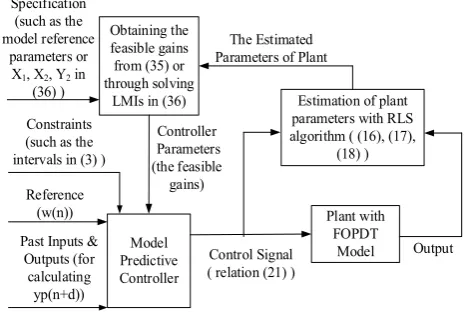
The general structure of the proposed adaptive MPC tuning strategy is shown in Fig. 1.
4- Simulation Results
In this section, three examples are used to verify the proposed adaptive tuning method. In the first example, a FOPDT plant is used with varying parameters. In the second example, the nonlinear pH process is considered and, finally, in the third
example, a second-order plant whose parameters vary is considered.
4- 1- Example 1
Consider the following FOPDT process [6]
( )
1.5e4 . 10 1s P
G s s
− =
+
Let Ts = 1sec. The related discrete transfer function is
( )
51
1
0.1425 . 1 0.905
P
z
G z− z−
−
= −
Let the desired closed-loop performance has a maximum Model
Predictive Controller
Plant with FOPDT
Model Estimation of plant parameters with RLS algorithm ( (16), (17),
(18) ) The Estimated Parameters of Plant
Output Obtaining the
feasible gains from (35) or through solving
LMIs in (36) Specification
(such as the model reference
parameters or X1, X2, Y2 in
(36) )
Reference (w(n)) Past Inputs &
Outputs (for calculating
yp(n+d))
Control Signal ( relation (21) ) Constraints
(such as the intervals in (3) )
Controller Parameters (the feasible
gains)
overshoot of 10% and a settling time of 14 sec up to 24 sec. A transfer function that satisfies these requirements can be
( )
51
1 2
0.1 ,
1 1.505 0.6048
d z z
z G
z
− −
− + −
= −
which is selected as the desired reference model. It is assumed that the plant parameters are unknown. Assume a 30% change in the parameter k at the time 300 sec and also a 50% change for parameter a at the time 800 sec occur. First, we apply the non-adaptive MPC tuning [6]. Fig 2 shows the results. We can see that although for the 30% variation of the parameter k in 300 sec, tracking is accetable (and only we have a small overshoot for a short time) but for 50% variation
of parameter a in 800 sec, the non-adaptive MPC cannot
track the reference signal.
Now, we apply the proposed adaptive MPC tuning strategy, and the results are shown in Figs 3, 4 and 5. In Fig. 3 it is shown that, the parameters of the system have converged to their real values after few seconds. Also, it can be seen that in Figs. 3a and 3b, the sudden variation of each parameter
k and a temporarily affects the other one. In this example,
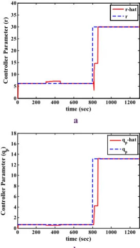
forgetting factor is selected as 0.96. In Fig. 4 the controller parameters are shown and we can see that they have positive values and are therefore acceptable. Since parameters r and
P
q according to (14) only include the system parametera
, they have not been affected by the change of parameter
k, and only their estimations were affected within the
transient time. Note that in this example, because the model of the plant is known (while in real applications the model is unknown with unknown variation), we can obtain the accurate controller parameters. Thus, in Fig 4, it has been shown that through the proposed adaptive MPC tuning method, the accurate controller parameters can be followed by any variation in the plant model parameters. Fig. 5 shows the closed-loop responses for the proposed adaptive MPC tuning method. The efficiency of the proposed method is shown in this figure and it can be seen that the sudden variation in 300 and 800 sec have been handled with very small overshoots.
a 0 200 400 600 800 1000 1200
-1.5 -1 -0.5 0 0.5 1 1.5 2
time (sec)
O
ut
put
Output Desired Output Reference
b 0 200 400 600 800 1000 1200
-1.5 -1 -0.5 0 0.5 1 1.5
time (sec)
Con
tr
ol
S
ign
al
Fig. 2. The closed-loop responses in example 1 (tuning method of [6]), a:Closed-loop Output, b: Control Signal.
0 200 400 600 800 1000 1200
0 5 10 15 20 25 30 35 40
time (sec)
C
on
tr
ol
ler
P
ara
m
et
er
(r
) r-hatr
a
0 200 400 600 800 1000 1200
0 2 4 6 8 10 12 14 16 18
time (sec)
C
on
tr
ol
ler
P
ara
m
et
er
(qp
) qqpp-hat
b
Fig. 4. The estimated MPC tuning parameters, a: predictive controller parameter r, b: predictive controller parameter qp.
20 40 60 80 100
0 1 2 3 4
5 d
time (sec)
D
ela
y
a
0 200 400 600 800 1000 1200
0 0.2 0.4 0.6 0.8 1
time (sec)
T
ime
C
on
sta
nt
a
thetahat theta
b
0 200 400 600 800 1000 1200
0 0.5 1 1.5 2 2.5
time (sec)
Ga
in
k
thetahat theta
c
4- 2- Example 2 (The Nonlinear pH Process)
Now, the proposed method is tested via the nonlinear pH process [17]. This process is a good benchmark to evaluate controllers. The dynamic and static equations of pH process can be found in [17]. Assume the following FOPDT model for the pH process in an operating point
( )
=0.9e100 1−30 +s P
G
s
s Ts=10sec→
( )
1 0.08565 41. 1 0.9048P z z
z
G − −
−
= −
Let K′xd1 and K′yd1 be selected as 0.7 and 0.148, respectively,
using the results of [6]. Fig. 6 shows the system output and the control signal in the case of non-adaptive tuning based on [6] and it can be seen that for the above constant FOPDT model, the non-adaptive MPC proposed in [6] is unable to control the neutralization pH process for the pH values 8 and 8.5. Now consider the proposed tuning method. It should be noted that the indirect RLS method for adapting this process is sensitive to the system parameters initial values. Fig. 7 shows the closed-loop responses of the adaptive proposed tuning method. It is shown that tracking performance is good. The effectiveness of the proposed tuning strategy is evident after comparing Figs. 6 and 7, and the control problem at pH values 8 and 8.5 in the non-adaptive MPC is resolved. 4- 3- Example 3 (Higher Order System)
In this example, a high-order plant is considered [19],
50
e
( ) ,
(150 1)(25 1)
P
s
G s
s s
−
=
+ +
where the corresponding discrete-time transfer function is 0 200 400 600 800 1000 1200 -2
-1.5 -1 -0.5 0 0.5 1 1.5 2 2.5
time (sec)
O
ut
put
Output Desired Output Reference
a
0 200 400 600 800 1000 1200 -4
-3 -2 -1 0 1 2 3
time (sec)
Con
tr
ol
S
ign
al
b
Fig. 5. The closed-loop responses in example 1 (Adaptive tuning method), a: Closed-loop output, b: Control Signal.
0.5 1 1.5 2 2.5
x 104
4 5 6 7 8 9 10 11 12
time(sec)
pH
Reference Output Desired Output
a
0.5 1 1.5 2 2.5 x 10⁴
10 15 20 25
time(sec)
Con
trol
S
ign
al
b
Fig. 6. Closed-loop responses for the pH process (tuning method [6]), a: Closed-loop output, b: Control Signal.
0.4 0.6 0.8 1 1.2 1.4 1.6 1.8 2 x 10⁴
4 5 6 7 8 9 10 11 12 13
time (sec)
pH
Output Reference Desired Output
a
0.4 0.6 0.8 1 1.2 1.4 1.6 1.8 2 x 10⁴
10 12 14 16 18 20 22
Con
trol
S
ign
al
time (sec) b
1 2
1 4
1 2
1 2
1 4 1 2 3
1 2
1 2
0.004378 0.02879 0.005041 ( )
1 1.482 0.5203
( ) .
1
p
p
z z
G z z
z z
b b z b z
G z z
a z a z
− −
− −
− −
− −
− −
− −
+ +
= →
− +
+ +
=
+ +
A proper approximated FOPDT model for this plant is given in [6] which shows that this high-order plant can be approximated by a FOPDT model with an acceptable error. Hence, in the proposed adaptive MPC method an estimated FOPDT model is derived. It is assumed that all parameters varies as: a1multiplies in 0.9 at 800 sec., a2 multiplies in 1.05 at 1200 sec., b1 multiplies in 5 at 1600 sec., b2
multiplies in 10 at 2100 sec., and b3 multiplies in 0.05 at 2600 sec.
Fig. 8 shows the system output and the control signal for the non-adaptive tuning method of [6] and Fig. 9 shows the same plots for the proposed adaptive MPC tuning method in this paper. It is seen that for the variation of the denominator parameter a1 at 800 sec., the response of the non-adaptive method is slow compared to the same response of the adaptive method. Also, at 2100 sec., with the variation of the
parameter b2, the response of the non-adaptive method is
unstable while the same response for the adaptive method is stable and yields a good tracking after some seconds. Thus, the effectiveness of the proposed method can be concluded for this high order time-varying plant.
0 500 1000 1500 2000 2500 3000 3500 -3
-2 -1 0 1 2 3
time (sec)
O
ut
put
Output Desired Output Reference
a
0 500 1000 1500 2000 2500 3000 3500 -5
0 5
time (sec)
C
on
tr
ol
S
ign
al
b
Fig. 8. Closed-loop responses for the second-order plant in example 3 (tuning method [6]), a: Closed-loop Output, b:
Control Signal.
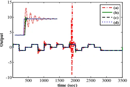
4- 4- Comparison of the proposed adaptive tuning method with a well-known online MPC tuning method
In this section, in order to investigate the advantages of the proposed tuning method, a comparison between the proposed method and an online tuning method [9] is presented. For
example, consider that a 30% decrement in the parameter a
and a 50% decrement in the parameter k occur at 800 sec. and also a 5% increment in the parameter a and a 20% increment
in the parameter k occur at 1800 sec. Fig. 10 shows the
result of the comparison between the online tuning method in [9] with the proposed adaptive tuning method in this paper. It shows that the reaction of the online tuning method to the system dynamic changes is more than the proposed method in this paper and the obtained response from the method of [9] is not desirable. Also, note that in the proposed online tuning method in [9], the initial plant model must be available and the online method of [9] can be affected just by unpredicted disturbances and unknown model parameters variations, while the proposed method in this paper does not need the initial plant model.
Note that the proposed method in this paper can be used either in the case that the plant model is unknown and time-varying or in the case that an unknown disturbance is applied to input or output. In these two cases, the new parameters of the FOPDT model are identified in each sampling time and for the desired closed-loop output, the tuning parameters of the predictive controller are obtained.
0 500 1000 1500 2000 2500 3000 3500 -3
-2 -1 0 1 2 3
time (sec)
O
ut
put
Output Desired Output Reference
a
0 500 1000 1500 2000 2500 3000 3500 -5
0 5
time (sec)
C
on
tr
ol
S
ign
al
b
Fig. 9. Closed-loop responses for the second-order plant in example 3 (proposed adaptive MPC tuning method in this
5- Conclusion
In this paper, an adaptive MPC tuning method was proposed based on the results of an available analytical MPC tuning method. Using RLS algorithm, we tried to update the tuning and controller parameters. Furthermore, an idea of the LMI was implemented when the obtained gains from the RLS algorithm were not feasible. Thus, in an algorithm, the proposed adaptive MPC tuning method was provided. Simulation results evaluated the effectiveness of the proposed method. Finally a comparison of the proposed
adaptive tuning method with a well-established online tuning method was briefly done.
In this paper, it was shown that the proposed adaptive tuning method can be used for all unknown time-varying arbitrary order systems which can be approximated by a FOPDT model. However, the proposed method is inefficient when the feasible gains cannot be reached for a special desired output. Also, since in the proposed method, the parameters of a FOPDT model must be estimated in each sampling time and the mentioned multiple LMIs must be solved, the calculation time for this method shall be reduced in a direct adaptive tuning case which will be considered in future studies by the authors.
References
[1] M.L. Darby, M. Nikolaou, MPC: Current practice and challenges, Control Eng. Pract, 20(4) (2012) 328-342. [2] D.Q. Mayne, Model predictive control: Recent
developments and future promise, Automatica, 50(12)
(2014) 2967-2986.
[3] J.L. Garriga, M. Soroush, Model predictive control
tuning methods: A review, Ind. Eng. Chem. Res, 49(8)
(2010) 3505-3515.
[4] P. Bagheri, A. Khaki-Sedigh, Tuning of dynamic matrix controller for FOPDT models using analysis of variance,
Proc. 18th IFAC World Congress, 44(1) (2011)
12319-12324.
[5] P. Bagheri, A. Khaki-Sedigh, Robust tuning of dynamic matrix controllers for first order plus dead time models,
Appl. Math. Model, 39(22) (2015) 7017-7031.
[6] P. Bagheri, A. Khaki-Sedigh, K.J.I.C.T. Sedigh, Applications, Analytical approach to tuning of model predictive control for first-order plus dead time models,
IET Control Theor. Appl,7(14) (2013) 1806-1817.
[7] P. Bagheri, A. Khaki-Sedigh, Closed form tuning equations for model predictive control of first-order plus fractional dead time models, Int. J. Control Autom. Syst, 13(1) (2015) 73-80.
[8] P. Bagheri, A. Khaki-Sedigh, An analytical tuning approach to multivariable model predictive controllers,
J. Process. Control, 24(12) (2014) 41-54.
[9] A. Al-Ghazzawi, E. Ali, A. Nouh, E. Zafiriou, On-line
tuning strategy for model predictive controllers, J.
Process Control, 11(3) (2001) 265-284.
[10] E. Ali, A. Al‐Ghazzawi, On‐line tuning of model
predictive controllers using fuzzy logic, Can. J. Chem.
Eng., 81(5) (2003) 1041-1051.
[11] E. Ali, Heuristic on-line tuning for nonlinear model
predictive controllers using fuzzy logic, J. Process
Control, vol, 13(5) (2003) 383-396.
[12] J. Van der Lee, W. Svrcek, B. Young, A tuning algorithm for model predictive controllers based on genetic algorithms and fuzzy decision making, ISA Trans., 47(1) (2008) 53-59.
[13] G. Valencia-Palomo, J. Rossiter, Programmable logic controller implementation of an auto-tuned predictive control based on minimal plant information, ISA Trans.,
50(1) (2011) 92-100.
[14] Q.N. Tran, J. Scholten, L. Ozkan, A. Backx, A model-free approach for auto-tuning of model predictive control,
Preprints of the 19th World congress, The International Federation of Automatic Control, Cape Town, South Africa,47(3) (2014) 2189-2194.
[15] S. Boyd, L. El-Ghaoui, E. Feron, V. Balakrishnan, Linear matrix inequalities in system and control theory,
SIAM,, 85(4) (1997) 698-699.
[16] C. Lynch, G. Dumont, Control loop performance monitoring, Control Syst. Technol, 4(2) (1996) 185-192. [17] M.A. Henson, D.E. Seborg, Adaptive nonlinear control
of a pH neutralization process, IEEE Trans. Control Syst. Technol, 2(3) (1994) 169-182.
[18] C. Bordons, E.F. Camacho, A generalized predictive controller for a wide class of industrial processes, IEEE Trans. Control Syst. Technol., 6(3) (1998) 372-387. [19] R. Shridhar, D.J. Cooper, A tuning strategy for
unconstrained SISO model predictive control, Ind. Eng.
Chem. Res., 36(3) (1997) 729-746.
500 1000 1500 2000 2500 3000 3500 -10
-5 0 5 10 15
time (sec)
O
ut
put
(a) (b) (c) (d)
Fig. 10. Closed-loop outputs for the FOPDT process of example A: (a) Output for the method of [9], (b) Output for the adaptive tuning method proposed in this paper, (c) Desired Output, (d)
Reference input.
Pleasecitethisarticleusing:
T. Gholaminejad, A. Khaki-Sedigh, P. Bagheri, Adaptive Tuning of Model Predictive Control Parameters Based on Analytical Results, AUT J. Model. Simul., 50(2) (2018) 109-116.
![Fig. 6. Closed-loop responses for the pH process (tuning method [6]), a: Closed-loop output, b: Control Signal.](https://thumb-us.123doks.com/thumbv2/123dok_us/8944124.1853492/6.595.338.522.419.708/closed-responses-process-tuning-method-closed-control-signal.webp)
![Fig. 8 shows the system output and the control signal for the non-adaptive tuning method of [6] and Fig](https://thumb-us.123doks.com/thumbv2/123dok_us/8944124.1853492/7.595.62.253.403.720/fig-shows-output-control-signal-adaptive-tuning-method.webp)